The degeneracy between the dust colour temperature and the spectral index

Abstract

Context. With the current Herschel and Planck satellite missions, there is strong interest in the interpretation of the details of the sub-millimetre dust emission spectra from interstellar clouds. A lot of work has been done to understand the negative correlation observed between the spectral index $\beta_{\rm Obs}$ and the colour temperature $T_{\rm C}$ that in the $\chi^{2}$ fits is partly caused by the observational noise.

Aims. In the ($T_{\rm C}$, $\beta_{\rm Obs}$) plane, the confidence regions are elongated, banana-shaped structures. Previous studies have indicated that the errors may exhibit strongly asymmetric features that have important consequences for the investigation of individual objects and the interpretation of the relation between the $T_{\rm C}$ and $\beta_{\rm Obs}$ parameters. We study under which conditions the confidence regions exhibit such anomalous, strongly non-Gaussian behaviour that could affect the interpretation of the observed ($T_{\rm C}$, $\beta_{\rm Obs}$) relations.

Methods. We examined a set of modified black body spectra and spectra calculated from radiative transfer models of filamentary interstellar clouds. We analysed simulated observations at discrete wavelengths between 100 $\mu$m and 850 $\mu$m. We performed modified black body fits and examined the structure of the $\chi^{2}(T_{\rm C},\beta_{\rm Obs})$ function of the fits.

Results. We demonstrate cases where, when the signal-to-noise ratio is low, the $\chi^{2}$ has multiple local minima in the $(T_{\rm C},\beta_{\rm Obs})$ plane. A small change in the weighting of the data points can cause the solution to jump to completely different values. In particular, if there is noise, the analysis of spectra with $T>10$ K and $\beta_{\rm Obs}\la 2$ can lead to a separate population of solutions with much lower colour temperature and higher spectral indices. The anomalies are caused by the noise. However, the tendency to show multiple $\chi^{2}$ minima depends on the model (in part via the influence on the signal-to-noise ratios) and on the set of wavelengths included in the analysis. Deviations from the underlying assumption of a single modified black body spectrum are not significant.

Conclusions. The presence of several local minima implies that the results obtained from the $\chi^{2}$ minimisation depend on the starting point of the optimisation and may correspond to non-global minima. Because of the strongly non-Gaussian nature of the errors, the obtained $(T_{\rm C},\beta_{\rm Obs})$ distribution may be contaminated by a few solutions with unrealistically low colour temperatures and high spectral indices. Proper weighting must be applied to avoid the determination of the $\beta_{\rm Obs}(T_{\rm C})$ relation to be unduly affected by these measurements.

1 Introduction

Observations of the thermal dust emission is one of the main methods used to map dense interstellar clouds. Sub-millimetre and millimetre emission is considered one of the most reliable ways of obtaining information about cloud cores in the different stages of the star formation process, from starless cores to protostellar systems (Motte et al. 1998; Andre et al. 2000; Enoch et al. 2007). To a large extent, this conclusion is based on the problems with the other tracers, i.e., the difficulty of interpreting molecular line data of the very dense clouds and the difficulty of assembling high-resolution maps using dust extinction or scattering (Lombardi et al. 2006; Goodman et al. 2009; Juvela et al. 2008, 2009).

The main difficulties in the interpretation of dust emission are well known. Because of the line-of-sight temperature variations, the peak of the emission spectrum becomes wider and this results in a decrease of the observed spectral index $\beta_{\rm Obs}$ (Shetty et al. 2009b; Malinen et al. 2011; Juvela & Ysard 2011). At the same time, because the observed emission is dominated by the warmer dust components within the beam, the colour temperature $T_{\rm C}$ overestimates the mass averaged physical dust temperature. This can lead to a significant underestimation of the dust mass (Evans et al. 2001; Stamatellos & Whitworth 2003; Malinen et al. 2011; Ysard et al. 2011). Furthermore, it is difficult to estimate the intrinsic dust grain properties, such as the spectral index, on the basis of the observed radiation.

When far-infrared and sub-millimetre observations are fitted with modified black body spectra, the dust colour temperature, $T_{\rm C}$, and the dust spectral index, $\beta_{\rm Obs}$, are partially degenerate. A small increase in $T_{\rm C}$ can be compensated by a small decrease of $\beta_{\rm Obs}$. When the observations contain noise, the ($T_{\rm C}$, $\beta_{\rm Obs}$) values will scatter over an elongated ellipse with a negative correlation between the two parameters. If the noise is large enough, the points will fall on a banana-shaped region where the $\beta_{\rm Obs}(T_{\rm C})$ relation becomes steeper at lower values of $T_{\rm C}$ (Shetty et al. 2009b, a; Veneziani et al. 2010; Paradis et al. 2010; Juvela et al. 2011). The common assumption is that apart from the curvature of the error banana, the scatter is symmetric with respect to the true values of $T_{\rm C}$ and $\beta_{\rm Obs}$ so that the expectation values do not show significant bias.

The $\beta_{\rm Obs}(T_{\rm C})$ relation induced by the noise is usually steeper than the average $\beta_{\rm Obs}(T_{\rm C})$ relation derived from observations of a large number of individual objects (Dupac et al. 2003; Désert et al. 2008; Planck Collaboration et al. 2011). If the average of the observed ($T_{\rm C}$, $\beta_{\rm Obs}$) points remains on the intrinsic $\beta(T)$ relation and if one observes a wide range of objects with different true temperatures, the effect of the bias can be controlled. However, there are some indications that under certain conditions, the error distribution is not symmetric and could behave in an even more non-Gaussian fashion (Planck Collaboration et al. 2011; Ysard et al. 2011). Under some conditions, the $\beta_{\rm Obs}(T_{\rm C})$ can extend to low colour temperatures and very high values of the spectral index. This could be important for the interpretation of the observed $\beta_{\rm Obs}(T_{\rm C})$ relations and, more generally, any attempt to measure cloud masses and temperatures using noisy continuum data.

In this paper we investigate this question by analysing noisy modified black body spectra, mixes of these spectra with different colour temperature, and spectra obtained from radiative transfer modelling of optically thick clouds. The content of the paper is the following. In Sect. 2 we describe the methods used to produce the spectra and to derive the colour temperature and the spectral index estimates. The main results are presented in Sect. 3. We start by looking at spectra calculated for optically thick filaments and by identifying the cases where the $\chi^{2}$ has more than one local minimum. In the Sect. 3.2 we return to modified black body spectra in an effort to identify the basic requirements for these anomalies. In Sect. 4 we discuss our results and the final conclusions are presented in Sect. 5.

2 Methods

We describe below the procedures used to calculate synthetic spectra and to derive the $T_{\rm C}$ and $\beta_{\rm Obs}$ values through $\chi^{2}$ minimisation.

2.1 Spectra from radiative transfer models

The first set of model spectra was obtained from the radiative transfer models discussed in Ysard et al. (2011). The models consist of optically thick filaments that are represented by long cylinders with radial density distributions following the ‘Plummer-like’ profiles (Nutter et al. 2008; Arzoumanian et al. 2011), which are flat at the centre of the filaments and decrease as $R^{-2}$ in the outer regions ($R$ is the radius of the clouds). The central extinction is varied in the range $A_{\rm V}=$1–20^m and the analysed sub-millimetre emission remains optically thin. The clouds are externally heated by the standard radiation field, ISRF (Mathis et al. 1983). Because cloud cores are often embedded in large molecular cloud complexes, this radiation field can also be attenuated corresponding to an external layer of dust with $A_{\rm V}^{\rm ext}=$1–5^m. We used dust properties representative of the dust in diffuse high Galactic latitude medium (DHGL) as defined in the DustEM dust models (Compiègne et al. 2011). The dust model consists of three dust populations: interstellar PAHs, amorphous carbons, and amorphous silicates. In the model clouds, the dust temperatures range from over 20 K for the amorphous carbon at the cloud surface to less than 10 K for the silicate grains at the centre of the filament, also depending on the model optical depth. Because of the wide range of temperatures and the different intrinsic emissivity spectral indices $\beta$ of the dust populations, the spectra cannot be fitted precisely with a single modified black body. For details of the calculations see Ysard et al. (2011).

2.2 Modified black body spectra

We additionally examined spectra that are based on modified black bodies to which observational noise is added. The different cases are (1) a single modified black body with a fixed value of $\beta$, (2) the sum of two modified black bodies with the same $\beta$ but different temperatures, and (3) a modified black body with different $\beta$ values below and above the wavelength of 500 $\mu$m. In the first scenario we are testing if the noise alone can produce a tail of solutions with high $\beta_{\rm Obs}$ and low $T_{\rm C}$ values. With the other modifications, we tested if the probability of extreme values is enhanced when the original spectrum cannot be described exactly as a single modified black body.

2.3 Analysis of the simulated spectra

In accordance with recent observational studies, we used measurements at a few far-infrared and sub-millimetre wavelengths. To simulate the Planck studies, we used the wavelengths of 350, 550, and 850 $\mu$m complemented with the 100 $\mu$m point that would be available from the IRAS survey (e.g., Planck Collaboration et al. 2011). As a default, we added to the spectra observational noise that is 0.06, 0.12, 0.12, and 0.08 MJy sr^-1 at the wavelengths of 100, 350, 550, and 850 $\mu$m, respectively. For Planck the uncertainties of the absolute surface brightness measurements are significantly smaller but these numbers are more realistic if the flux determination includes the separation of a background component (see Planck Collaboration et al. 2011). To simulate Herschel observations, we used the wavelengths of 100, 160, 250, 350, and 500 $\mu$m (e.g., Paradis et al. 2010; Juvela et al. 2011) with noise levels of 8.1, 3.7, 1.2, 0.85, and 0.35 MJy sr^-1 per beam. In the analysis the data are convolved to the resolution of the 500 $\mu$m observations and this results in final uncertainties of 1.62, 1.18, 0.60, 0.60, and 0.35 MJy sr^-1, respectively. After the beam convolution, the absolute signal is lower for the simulated Planck data (a resolution of $\sim 5\arcmin$) compared to the simulated Herschel data (a resolution of $\sim 36\arcsec$ at the wavelength of 500 $\mu$m). This reduces the difference in the signal-to-noise ratios (S/N) of the two data sets (see Fig. 1).

A weighted least-squares fit of a single modified black body ($\chi^{2}$ minimisation) was used to estimate the colour temperature $T_{\rm C}$ and the observed spectral index $\beta_{\rm Obs}$. The wavelength ranges fitted are 100–850 $\mu$m for the combined data of Planck and IRAS and 100–500 $\mu$m for the simulated Herschel data. The weighting was done with the actual noise in each channel although the effect of changing the weight of the 100 $\mu$m measurement was also examined. When there are temperature variations, the derived $T_{\rm C}$ and $\beta_{\rm Obs}$ values differ from the mass weighted average dust temperature and from the actual spectral index of the dust grains. However, in this paper we concentrate on the effects of noise. Therefore we concentrated on the question of how the $T_{\rm C}$ and $\beta_{\rm Obs}$ values differ from the values that would be obtained with a similar analysis of the noiseless spectra.

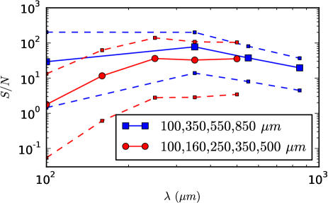
Figure 1: Signal-to-noise ratios in the simulated observations. The solid lines show the average and the dashed lines the minimum and the maximum S/N ratio as the function of wavelength.

3 Results

3.1 Spectra from radiative transfer models

3.1.1 Simulated Planck and IRAS observations

We start with a study of the spectra that were calculated in Ysard et al. (2011) for models of cloud filaments at a distance of $d$=100 pc. Figure 2 shows the ($T_{\rm C}$, $\beta_{\rm Obs}$) values derived from simulated observations of 100, 350, 550, and 850 $\mu$m with the default noise (see Sect 2.1). In the figure we include models with $A_{\rm V}$=10–20^m and with the ISRF attenuated by an external dust layers with $A_{\rm V}^{\rm ext}$=4–5^m. For these models the locus of the correct $T_{\rm C}$ and $\beta_{\rm Obs}$ values (i.e., the parameters estimated in the absence of noise) is between the $T_{\rm C}$ values of 12.0 K and 12.8 K and the $\beta$ values 1.02 and 1.11. Because of the noise the estimates scatter along a narrow banana-shaped region. Most points cluster around the median value of 12.47 K and $\beta$=1.07. The figure contains 10000 points of which 217 are below $T_{\rm C}$=8 K.

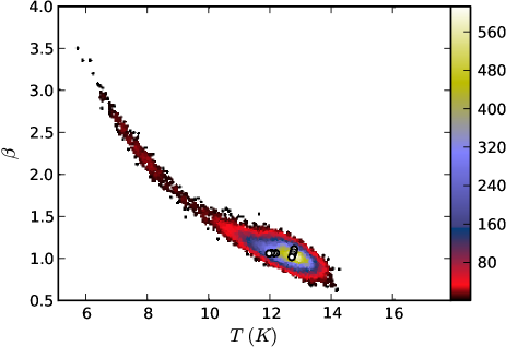
Figure 2: Distribution of ($T_{\rm C}$, $\beta_{\rm Obs}$) values for the modified black body fits of the spectra calculated for the filament models. The colour scale shows the density of points per $\Delta T_{\rm C}$=0.2 K and $\Delta\beta_{\rm Obs}$=0.1. The white circles (with black borders) indicate the values obtained for the examined models in the absence of noise.

The histograms in Fig. 3 show that the parameter distributions are not symmetric and this is not caused merely by the curvature of the confidence region. The colour temperature distribution has a tail towards low values and a secondary peak is visible around 7–8 K. The spectral index distribution is correspondingly skewed in the other direction with a tail extending to high values of $\beta$. Altogether 4.6% of the points have $T_{\rm C}<10$ K. These represent a strongly non-Gaussian part of the error distribution that, if not properly accounted for, would negate any attempts to determine what the real $\beta_{\rm Obs}(T_{\rm C})$ dependence would be in the absence of noise.

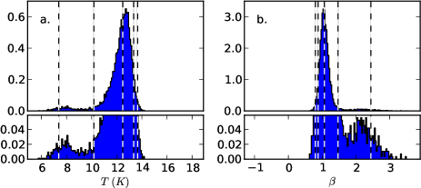
Figure 3: Marginal distributions (i.e. the probabilities integrated over the $\beta$ and $T_{\rm C}$ axes, respectively) of the points in Fig. 4. The upper frames show the probability density distributions of the $T_{\rm C}$ and $\beta$ parameters and the lower frames show a zoomed version of the upper frames. The histograms have been normalised to represent probability distributions (area normalised to one). The vertical dashed lines indicate the median of the distribution and the points where the tails of the distribution (one-sided) contain 5% or 1% of the data.

For filament models of lower $A_{\rm V}$ and thus of lower signal-to-noise ratio the high $\beta_{\rm Obs}$ solutions become more common. The $A_{\rm V}=20^{\rm m}$ models are responsible for $\sim$17% of all the points below $T_{\rm C}=8$ K, while the contribution of the clouds with a central $A_{\rm V}$ of $10^{\rm m}$ is already over 26%. More interestingly, the long tail to low colour temperatures is almost exclusively produced by the models where the external radiation field is attenuated by a dust layer of $A_{\rm V}^{\rm ext}=5^{\rm m}$. The models with $A_{\rm V}^{\rm ext}=4^{\rm m}$ still show an asymmetry of the $T_{\rm C}$ distribution but their contribution to the tail below $T_{\rm C}=10.0$ K is only a couple of percent. Figure 2 also shows the ($T_{\rm C}$, $\beta_{obs}$) values that would have been obtained from the various models if there were no observational noise. The $A_{\rm V}^{\rm ext}=4^{\rm m}$ and $A_{\rm V}^{\rm ext}=5^{\rm m}$ models form separate groups, the latter being colder, as measured by the noiseless colour temperature, by $\Delta T_{\rm C}\sim$1 K. The higher $A_{\rm V}^{\rm ext}$ values reduce the physical dust temperature especially at the cloud surface. The effect is felt most strongly at 100 $\mu$m where the signal-to-noise ratio drops by $\sim$40% (from $\sim$6 down to $\sim$3.5, almost irrespective of the central $A_{\rm V}$ of the model cloud).

Figure 4 shows one example of a $A_{\rm V}=5^{\rm m}$ cloud where the surface brightness values are 0.088, 1.62, 1.27, and 0.35 MJy sr^-1 at the wavelengths 100, 350, 550, and 850 $\mu$m, respectively. A fit to the original noiseless data gives values $T_{\rm C}=$12.6 K and $\beta_{\rm Obs}$=1.14. With this particular noise realisation the $\chi^{2}$ minimum has moved to $T_{\rm C}$=4.78 K and $\beta_{\rm Obs}=$4.46. These values are suspicious because the colour temperature is well below the minimum dust temperature of the model cloud, which is always higher than 8 K. The spectral index $\beta_{\rm Obs}$ is also higher than the dust intrinsic $\beta$ (1.55 and 2.11 for amorphous carbons and silicates, respectively, see Fig.8 in Ysard et al. 2011) although it would be expected to be lower because of the line-of-sight temperature variations. In the model clouds the actual dust temperature does not decrease below $\sim$8 K, while the spectral indices of the dust grains only are 2.11 for astronomical silicates and 1.55 for amorphous carbon grains (see Fig. 8 in Ysard et al. 2011).

In this case the 100 $\mu$m intensity was not much more than 1-$\sigma$ detection. However, the 100 $\mu$m value happens to be almost identical to the correct noiseless value. On the other hand, the 550 $\mu$m observation is almost 2.5$\sigma$ above the correct value. This is the main reason for the very low temperature. The contour plot of the $\chi^{2}$ values (lower frame in Fig. 4) shows that the confidence region is very elongated. The ‘correct’ solution (i.e., the one for the noiseless spectrum) resides in the $\chi^{2}$ valley but with a $\chi^{2}$ value that is four times the $\chi^{2}$ value of the best fit.

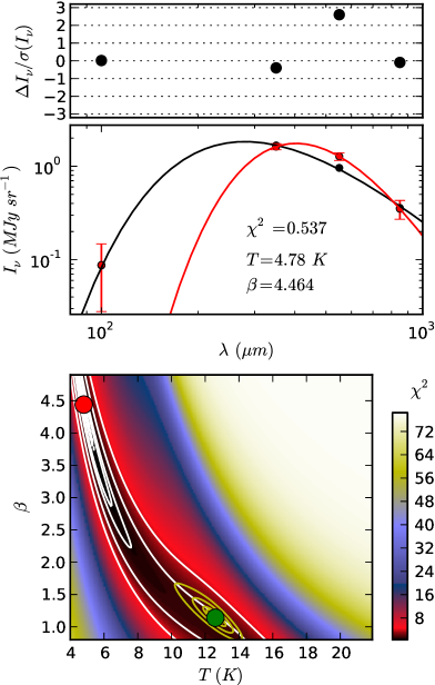
Figure 4: Case where noise has resulted in a high $\beta$ value. In the middle frame, the black curve is the spectrum obtained from the cloud modelling. The red symbols are the measurements that include noise and the red curve is the fit to these points. The uppermost frame shows the deviations $\Delta I_{\nu}$ (the difference between the simulated observation and the fit) in units of the assumed uncertainty $\sigma I_{\nu}$. The bottom frame shows the $\chi^{2}$ values as a function of $T_{\rm C}$ and $\beta_{\rm Obs}$. The colour plot and the white contours show the $\chi^{2}$ values for the fit to the noisy data. The contours are drawn at 1.02, 1.05, 1.1, 1.5, 2.0, 4.0, and 8.0 times the minimum $\chi^{2}$ value. In yellow are shown the corresponding contours for the fit to the noiseless data. The two circles denote the locations of the $\chi^{2}$ minima with (red circle) and without (green circle) the noise.

If the observations do not perfectly fit a single modified black body, the best fit will depend on the relative weight given to the individual measurements. Figure 5 shows that interesting changes take place when the assumed uncertainty of the 100 $\mu$m point is decreased by a factor of $\sim$0.57. The measured values (including the noise) are not changed and only the weight of the 100 $\mu$m point is increased in the fit. In the present example the 100 $\mu$m value happens to be almost correct. Therefore, the error estimates could be decreased much more than by a factor of 0.57 without this particular noise realisation becoming improbable. In Fig. 5 the 100 $\mu$m noise is scaled by 0.575 in the left hand frames and by 0.570 in the right hand frames. As the weight of the 100 $\mu$m point is modified, the $\chi^{2}$ minimum jumps instantaneously from the high $\beta$ solution to a solution near the value of the original noiseless spectrum. At this point the signal-to-noise ratio of the 350 $\mu$m data point is $\sim$18. The $\chi^{2}$ values are almost identical, the change being consistent with the effect of the very small decrease of the 100 $\mu$m uncertainty. The parameter space was sampled with intervals $\Delta T$=0.1 K and $\Delta\beta$=0.02.

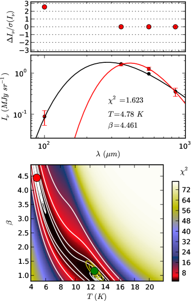
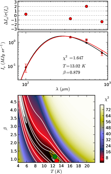
Figure 5: As Fig. 4 but assuming in the fit a 100 $\mu$m uncertainty that is 0.575 times (frames on the left) or 0.570 times (frames on the right) the original value. The intensity values are the same as before. The $\chi^{2}$ plane exhibits two distinct local minima and a small change in the weight of the 100 $\mu$m measurement moves the solution from a high $\beta$ solution to a low $\beta$ solution.

The example reveals some important facts. Firstly, the solution based on $\chi^{2}$ minimum can change significantly and in a non-continuous fashion when the measured intensities or the assumed uncertainties are slightly perturbed. Secondly, the presence of multiple local $\chi^{2}$ minima implies that the solution obtained by non-linear optimisation will depend on the initial values of the optimisation. The obtained result may correspond to a local instead of a global minimum. Thirdly, as already indicated in Fig. 3, the error distributions are skewed and possibly even bimodal. This has implications not only for the uncertainties of the $\chi^{2}$ approach but more generally for the statistical models employed in other parameter estimation methods.

In the following we call ‘normal’ the solution that is close to the values obtained in the absence of noise and ‘anomalous’ the solutions that exhibit a significantly lower value of $T_{\rm C}$ and a higher value of $\beta_{\rm Obs}$. Another example is shown in Appendix A where the 550 $\mu$m point is more than 2$\sigma$ above the correct (noiseless) value. In the 217 cases of the $A_{\rm V}\geq 10^{\rm m}$ model spectra with colour temperature below 8 K ($\sim$2% of all spectra), the common feature is that the 550 $\mu$m point is high relative to the neighbouring wavelengths and especially relative to the 850 $\mu$m point. This is demonstrated in Fig. 6 which shows the differences between the observed and the true intensities when the estimated $T_{\rm C}$ was below 8 K. With a low weight of the 100 $\mu$m measurement, a solution with a very high value of $\beta_{\rm Obs}$ becomes possible. The anomalous solutions are seen more frequently but not exclusively when the 100 $\mu$m intensity is underestimated. One must also note that the previous colour temperature estimates (e.g., Fig. 2) were based on $\chi^{2}$ optimisation where the initial values, $T=$15 K and $\beta$=1.5, favoured the high-temperature solution.

It is time-consuming to estimate the $\chi^{2}$ values for the modified black body fits with a dense grid over the whole ($T_{\rm C}$, $\beta$) plane. Instead, to identify the cases with two $\chi^{2}$ minima, we started non-linear optimisation (the Powell method) at two locations, ($T_{\rm C}$, $\beta$)=(7.0K, 4.0) and (13.0 K, 0.9). If two minima exist, the optimisation is likely (although not guaranteed) to converge to different values. With these two initial values the optimisation may still converge to the same local minimum, missing the second one. On the other hand, if there is only one very shallow minimum, the optimisations may produce different results for numerical reasons.

The presence of a single $\chi^{2}$ minimum does not tell us whether it corresponds to the normal or the anomalous solution. To see whether one is close to a situation where two $\chi^{2}$ minima appear, we also scaled the 100 $\mu$m error estimates by a factor $K_{\rm 100}$ that was changed from 0.5 to 1.5 in steps of 0.1. This way one can perturb the problem and obtain an indication whether the result of the fit is well-defined or not. As seen in Fig. 5, the minimum can shift very rapidly between the normal and the anomalous solution. The second local $\chi^{2}$ minimum exists only for few a $K_{\rm 100}$ values close to that point. Our emphasis is on the non-Gaussian nature of the uncertainties (as produced by the multiple minima). Note that for example Fig. 2 was obtained using only the original weighting of the data , $K_{100}=$1.0.

We examined the above set of 10000 spectra from cylindrical cloud models with $A_{\rm V}$=10–20^m and $A_{\rm V}^{\rm ext}$ of 4–5^m. This revealed $\sim$680 cases where different initial parameter estimates lead to different optimised values with $\Delta T>0.2$ or $\Delta\beta>0.1$. This happened preferentially when the 100 $\mu$m uncertainties were increased but could take place for any usually small range of $K_{100}$ values. In these models the ratio of the original intensity and the added noise was at 100 $\mu$m higher than 3.2, with an average value of 4.7. Of the three Planck channels the 500 $\mu$m band had the lowest ratio with a minimum of 15.1 and a mean value of 18.7. The actual signal-to-noise ratios can be lower when the observed intensity is below the expectation value of the intensity.

The double $\chi^{2}$ minima are caused by the noise but their frequency of appearance depends on the model, probably mainly through the associated changes in the signal-to-noise ratios of the observations. For the same model clouds with $A_{\rm V}$=10–20^m but with the external radiation field attenuated by $A_{\rm V}^{\rm ext}<4^{\rm m}$ rather than 4–5^m, the double minima become less frequent by a factor of ten. With $A_{\rm V}^{\rm ext}\leq 2^{\rm m}$ the solutions were unique, probably because of the higher surface brightness values of those models.

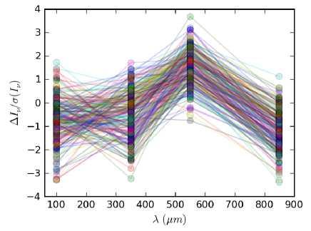
Figure 6: Errors in the observed intensities in the cases where the simulated Planck and IRAS 100 $\mu$m observations result in colour temperatures $T_{\rm C}<$8 K. The errors are given as the difference between the observed intensity and the noiseless spectrum, measured in units of the uncertainty assumed in the modified black body fits.

3.1.2 Simulated Herschel observations

The simulated Herschel observations consisted of the wavelengths of 100, 160, 250, 350, and 500 $\mu$m. Figure 7 shows the $(T_{\rm C},\beta)$ values for the models from Ysard et al. (2011) with the cloud central $A_{\rm V}$=10–20^m and an external $A_{\rm V}^{\rm ext}$=4–5. This is only a subset of all models discussed in Ysard et al. (2011). The original weighting of the 100 $\mu$m data has not been altered (i.e., $K_{\rm 100}=$1.0). The figure includes 10000 points out of which only 83 are below $T_{\rm C}$=9 K.

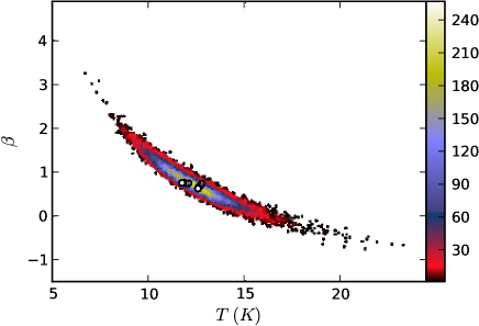
Figure 7: Distribution of $(T_{\rm C},\beta)$ for simulated Herschel observations. The colour scale gives the density of the points per $\Delta T_{\rm C}$=0.2 K and $\Delta\beta_{\rm Obs}$=0.1 The white circles (with black borders) indicate the values that would be obtained for the included models if there were no noise.

The scatter of the temperature and spectral index values is more symmetric than for the Planck+IRAS data set. This is confirmed in Fig. 8 which shows the marginal distributions where the $T_{\rm C}$ data have only a hint of a tail towards higher temperatures (skewness 0.63), i.e., opposite to the behaviour in Fig. 3. All spectra were again fitted using an optimisation with different initial values of $T_{\rm C}$ and $\beta$. Out of the 10000 spectra with $A_{\rm V}$=10–20^m and $A_{\rm V}^{\rm ext}$4–5^m, two $\chi^{2}$ minima were inferred only in a single case. This even though the 100 $\mu$m S/N ratios was below one and the 160 $\mu$m ratios only a few, the mean value being 5.0. For the longer wavelengths, the S/N ratios were $\sim$20 or above. The $\chi^{2}$ plane was examined for some of the cases with the lowest colour temperature to confirm the presence only of a single local minimum. The other two samples, the case with $A_{\rm V}$=10–20^V and $A_{\rm V}^{\rm ext}<4^{\rm m}$ and the case with $A_{\rm V}$=1^V and $A_{\rm V}^{\rm ext}<1^{\rm m}$, together contain only one additional case where two local $\chi^{2}$ minima were detected.

On the basis of the previous tests the appearance of anomalous solutions depends mainly on the noise. The comparison of the Planck and Herschel cases shows that the set of wavelengths included in the analysis is equally important. The uncertainties of the simulated Herschel observations are all higher in absolute terms but the relative uncertainty between the short and the long wavelengths is similar to the Planck case. The combination of five wavelengths appears to be resistant against extreme errors that could be caused, for example, by a 2-$\sigma$ or 3-$\sigma$ error in a single channel (cf. Fig.4). The $T_{\rm C}$ and $\beta_{\rm obs}$ distributions are wide because of the noise but there still are practically no values of $T_{\rm C}<8$ K.

There is still the possibility that the results could depend on how much the underlying spectrum deviates from a single modified black body. To further examine this question, we next examined a series of models based on modified black bodies.

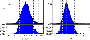
Figure 8: Probability distributions of $T_{\rm C}$ and $\beta$ for the simulated Herschel observations of Fig. 7 (for further details, see the caption of Fig. 3).

3.2 Modified black body spectra

We examined a series modified black body spectra $B_{\nu}(T)\times\nu^{\beta}$ together with noise to look for similar anomalous cases as shown in Fig. 5. Several combinations of the temperature and spectral index were investigated. We started with the 100 $\mu$m band and the three Planck bands 350–850 $\mu$m. When the modified black body spectra are scaled to have a 350 $\mu$m signal of 2.0 MJy sr^-1, the signal-to-noise ratio is comparable to that of Fig. 5. However, to examine the effect of different S/N ratios, the spectra were scaled by a factor that was varied from 0.6 to 6.0 in five logarithmic steps. To investigate the sensitivity to the relative weighting of the frequency points in the fit, we included the factor $K_{\rm 100}$ which was varied from 0.5 to 1.5. As before, the factor $K_{\rm 100}$ did not affect the noise, only the relative weighting of the data points in the fit. For each case (i.e., a combination of temperature, spectral index, the intensity scaling, and the value of $K_{\rm 100}$), we ran 5000 noise realisations of the spectrum. Each spectrum was fitted using the two different initial values of the optimisation to recognise the cases with separate $\chi^{2}$ minima.

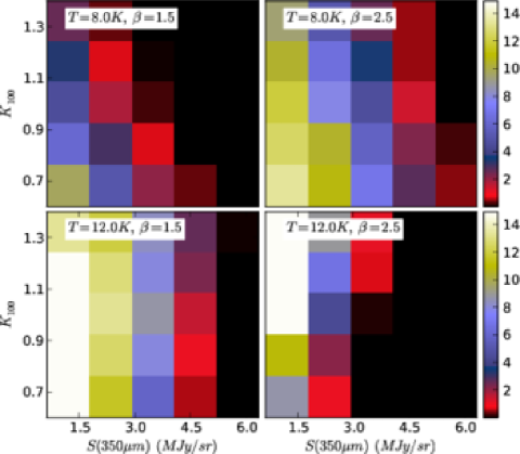
Figure 9: Frequency of recognised $\chi^{2}$ double minima for simulated IRAS and Planck observations. Each frame corresponds to one combination of the temperature and the spectral index that were inputs of the simulation. The horizontal axis gives the 350 $\mu$m intensity (before noise is added) and the vertical axis is the factor $K_{\rm 100}$ (smaller numbers correspond to a larger weight of the 100 $\mu$m point). The colour scale gives the frequency of the double $\chi^{2}$ minima as a percentage of all noise realisations with the corresponding values of $S(350\,mu{\rm m})$ and $K_{\rm 100}$.

Double minima are detected in $\sim$10% of the cases but the frequency drops close to zero by the time the S/N ratio is increased by a factor of three (Fig. 9). There is some dependence on the model in question but this may also be caused by the differences in the S/N ratios of the other bands. With $T=8.0$ K and $\beta=$1.5, the double minima are significantly more rare when the 100 $\mu$m data point is given a larger weight ($K_{\rm 100}<$1.0). With $T=12.0$ K and $\beta=$2.5, the opposite is true.

Figure 10 shows the corresponding results for the Herschel data that were scaled to have the same S/N ratios at the 350 $\mu$m wavelength as in the previous Planck examples (the observational uncertainties are the same as in Sect. 3.1). Distinct $\chi^{2}$ minima are observed only with $T_{\rm C}=8.0$ K and $\beta=1.5$ and even in that case the number is below 1%. When the signal-to-noise ratio is increased by a factor of three, no double minima are detected (probability $\sim 10^{-4}$ or less).

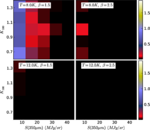
Figure 10: Frequency of recognised $\chi^{2}$ double minima for simulated Herschel observations. Each frame corresponds to one modified black body with the given temperature and the spectral index. The horizontal axis gives the 350 $\mu$m intensity (the S/N ratios are the same as in Fig.9) and the vertical axis is $K_{\rm 100}$, the relative weighting of the 100 $\mu$m point. The colour scale gives the frequency of the double $\chi^{2}$ minima as a percentage.

If the 350 $\mu$m signal of the simulated Herschel observations is lowered to 2.0 MJy sr^-1, the S/N ratios decrease by a factor of seven. As shown in Fig. 11, in this case the number of double minima increases to $\sim$10%, a level similar to the previous Planck example.

The figures in Appendix B show the bias and scatter of the $T_{\rm C}$ and $\beta_{\rm obs}$ values corresponding to the cases in Figs. 9–11.

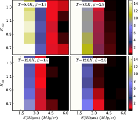
Figure 11: Frequency of the recognised $\chi^{2}$ double minima for simulated Herschel observations when the signal-to-noise ratio has been decreased by a factor of seven compared to Fig. 10.

We next examined spectra that are the sums of two modified black bodies that have the same spectral index but different temperatures, $I_{\nu}=(B_{\nu}(T_{1})+B_{\nu}(T_{2}))\times\nu^{\beta}$. The deviations from a single modified black body could make the fit more susceptible to ambiguity.

The results for the Planck+IRAS case are presented in Fig. 12. They look quite similar to the single black body cases shown in Fig. 9 where, of course, also the temperatures are somewhat different. It seems that the deviations from a single modified black body shape do not have a significant effect on the presence of multiple $\chi^{2}$ minima. The conclusion is confirmed by the Herschel simulations in Fig. 13, which is to be compared with Fig. 10. The differences are again small and may be mainly caused by the temperature differences, higher (average) temperatures leading to fewer cases of multimodal $\chi^{2}$ distribution.

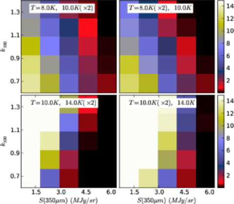
Figure 12: Frequency of the recognised double $\chi^{2}$ minima for the sum of two modified black bodies with temperatures 8 and 10 K or 10 and 14 K. The column density ratio of the lower temperature and the higher temperature component is 1:2 or 2:1, as indicated in the frames. The data correspond to simulated observations at 100 $\mu$m and three Planck wavelengths.

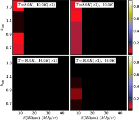
Figure 13: As Fig. 12 but for simulated Herschel observations.

As a final deviation from single modified black bodies we examined spectra where the spectral index is $\beta=2.0$ up to 300 $\mu$m and $\beta=1.5$ at the longer wavelengths. The break in $\beta$ does not cause any significant change in the number of double $\chi^{2}$ minima, either in the simulated Planck observations (Fig. 14 vs. Fig. 9) or in the simulated Herschel observations (Fig. 15 vs. Fig. 11).

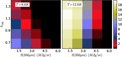
Figure 14: Frequency of the recognised double $\chi^{2}$ minima for the modified black bodies with a break in the spectral slope. The data correspond to simulated observations at 100 $\mu$m and three Planck wavelengths.

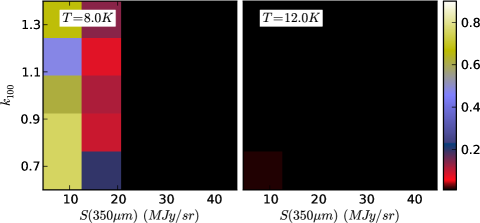
Figure 15: Frequency of the recognised double $\chi^{2}$ minima for the modified black bodies with a break in the spectral slope. The figure correspond to simulated Herschel data with the 350 $\mu$m S/N identical to that in the Planck case in Fig. 14.

4 Discussion

The tests with the grey body spectra showed that with four wavelengths 100, 350, 550, and 850 $\mu$m and signal-to-noise ratios similar to those in Fig. 5, the $\chi^{2}$ values of the modified black body fits exhibit multiple minima in up to $\sim$10% of the cases. This is similar to the fraction of ‘anomalous’ solutions that were seen for the radiative transfer models of cylindrical filaments ($T_{\rm C}<$10 K) in Figs. 2 and 3.

With the five wavelengths of 100, 160, 250, 350, and 500 $\mu$m the number of multiple $\chi^{2}$ minima was lower by a factor of $\sim$100 (see Fig. 11) when the 350 $\mu$m signal-to-noise ratio was similar to that of the previous case with four wavelengths (S/N$\sim$20). Therefore the better wavelength sampling provided by the set of five frequencies is the main reason for the disappearance of the double $\chi^{2}$ minima. With four wavelengths, the anomalous solutions always corresponded to a 350 $\mu$m value that was overestimated by $\sim 2\sigma$ relative to the neighbouring wavelengths (see Fig. 6). With five wavelengths, an anomalous solution might require a similar error in two neighbouring channels (e.g., 250 $\mu$m and 350 $\mu$m) that, for normally distributed errors and $2-\sigma$ deviations should be less likely by a factor of 50. The number of anomalous solutions increased to the 10% level only when the S/N ratios were decreased by a factor of six and the 350 $\mu$m S/N ratio was close to three.

Are the separate $\chi^{2}$ minima of practical importance? In the extreme cases like the one shown in Fig. 5, the multimodality of the $\chi^{2}$ values causes clear complications. When the minima are of similar depth, the result obtained by optimisation methods depends on the initial values. Furthermore, an infinitesimal change in the flux values or in their weighting can switch the global minimum between the low- and the high-temperature solution. The difference can be several degrees in colour temperature and several units in spectral index. Because of the strongly non-Gaussian behaviour of the problem the uncertainties deduced from the local shape of the $\chi^{2}$ surface will radically underestimate the true uncertainties of $T_{\rm C}$ and $\beta_{\rm Obs}$. In principle the problem can be avoided by calculating the $\chi^{2}$ values over the whole parameter plane. This is expensive but may also not yet be a completely satisfactory solution. The examples have shown that the shape of the $\chi^{2}$ surface can change rapidly as, for example, the error estimates are changed. In Sect. 3.2 we noticed that double minima could appear and again disappear when the factor $K_{\rm 100}$ was changed at a 10% level. This means that also the uncertainty of the flux uncertainties and their impact on the $\chi^{2}$ surface should be examined. However, the real error estimates are rarely known to a precision of 10%. On the positive side, many anomalous solutions may be recognisable from the SED plots. In Fig. 5 the low-temperature solution would certainly be treated with some caution, in spite of it corresponding to the lowest $\chi^{2}$ value. The situation becomes less clear when the distance between the minima is shorter. One should always take into account that for low signal-to-noise ratio data there is a non-negligible probability, possibly even in excess of $\sim$10%, that the deepest $\chi^{2}$ minimum is not the minimum closest to the true solution.

The problem is less tractable in large surveys of individual sources or maps with thousands of pixels. It becomes difficult to examine each SED fit by eye and the calculation of the full $\chi^{2}$ surfaces may become impractical. If not accounted for, even a few anomalous solutions can significantly affect the deduced shape of the $\beta(T)$ relation. One can use Monte Carlo methods to estimate the number and the influence of the outliers, including the effects of the non-Gaussian statistics (e.g. Planck Collaboration et al. 2011)). Conversely, one can try to directly recover the true $\beta(T)$ relation with Bayesian methods (Veneziani et al. 2010; Kelly et al. 2011). In those cases the multimodal $\chi^{2}$ distribution may not be a significant complication because the methods are aware of the shape of the likelihood function and that is additionally modified by the prior. However, an accurate knowledge of the statistics of the observed intensities is still needed.

To quantify the role of the double $\chi^{2}$ minima (as opposed to the general influence of noise) we examined again the simulated observations of Fig. 9. For each combination of $S(350\mu{\rm m})$ and $K_{\rm 100}$, we took 200 samples of ($T_{\rm C}$, $\beta_{\rm Obs}$) corresponding to the different temperatures used in the simulation (8.0, 10.0, and 12.0 K) and a fixed input spectral index of $\beta=2.0$. The resulting linear correlation coefficients between $T_{\rm C}$ and $\beta_{\rm Obs}$ are shown in Fig. 16$a$. In the absence of noise the correlation should be zero. The observed correlation varies from -0.5 (for the data with the highest signal-to-noise ratio) to $\sim$-0.8. Note that the correlation coefficient does not increase monotonously to the lowest S/N ratios because of the strong non-linearity of the $\beta_{\rm Obs}(T_{\rm C})$ relation. The frame $b$ of Fig. 16 shows the correlation coefficients excluding those cases where the $\chi^{2}$ shows two minima (for that particular value of $K_{\rm 100}$). The effect of the cases of double $\chi^{2}$ minima is visible at a 10% level.

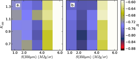
Figure 16: Linear correlation coefficients between $T_{\rm C}$ and $\beta_{\rm Obs}$ for the models of Fig. 9 as functions of the source intensity $S(350\mu{\rm m})$ and the weight given in the fit to the 100 $\mu$m point (lower value of $K_{\rm 100}$ implies a larger weight). Frame $b$ is the same after removing the points that correspond to the presence of multiple local $\chi^{2}$ minima.

The anomalous solutions may be identified by the unrealistic values of the colour temperature and the spectral index. However, the presence of multiple $\chi^{2}$ minima also directly serves as a warning sign. Figure 17 displays the distribution of the ($T_{\rm C}$, $\beta_{\rm Obs}$) values for the modified black body model with $T=12$ K and $\beta$=1.5 that had particularly many multiple minima (see Fig. 9). The points plotted in Fig. 17 corresponds to the solution obtained from optimisation with initial values close to the true solution. The figure shows 500 points for each value of $S(350\mu{\rm m})$, all corresponding to the default weighting with $K_{\rm 100}$=1.0. The blue points are the cases where two $\chi^{2}$ minima were detected with any of the tested $K_{\rm 100}$ values (see Sect. 3.2). The red points are a subset where double minima were detected with the present value of $K_{\rm 100}$=1.0. The blue points are seen to avoid the locus of the correct solution that still contains most of the data. Especially the red points are concentrated in the low-temperature tail. Of all the points below the colour temperature of 8 K, 42% corresponded to cases with multiple $\chi^{2}$ minima (or extremely shallow single minima that for numerical reasons lead to different parameter estimates). If the test is carried out using all $K_{\rm 100}$ factors between 0.5 and 1.5, the percentage increases to 70%. This suggests that similar tests should be useful also for real observations.

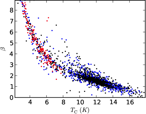
Figure 17: ($T_{\rm C}$, $\beta_{\rm Obs}$) values for simulated modified black bodies with $T=12$ K and $\beta=$1.5 (see Sect. 3.2). The data points correspond to the normal weighting of data ($K_{\rm 100}$=1.0) and to all S/N ratios shown in Fig. 9). The red points denote cases where double $\chi^{2}$ minima were detected with $K_{\rm 100}$=1.0 and the blue points the other cases where double minima were seen with any value of $K_{\rm 100}$ between 0.5 and 1.5

5 Conclusions

We have studied the behaviour of $\chi^{2}$ fits of SEDs that are either sums of modified black bodies or are based on the radiative transfer modelling of dust emission from cylindrical clouds. Using combinations of wavelengths relevant for the current Planck and Herschel satellite studies, we have examined the effect of noise on the shape of the confidence regions in the ($T_{\rm C}$, $\beta_{\rm Obs}$) plane.

The results have lead to the following conclusions:

• In addition to the usual symmetric error banana, the $\chi^{2}$ distribution can exhibit asymmetries of varying strength. The expectation values are close to the result obtained in the absence of noise, but are not without bias.

• For low signal-to-noise data (S/N below 10) in the 100 $\mu$m, 350 $\mu$m, 550 $\mu$m, and 850 $\mu$m bands, the noise distribution of ($T_{\rm C}$, $\beta_{\rm Obs}$) values develops an asymmetric tail that can extend to low temperatures and very high spectral indices.

• Under the same conditions, the $\chi^{2}$ distribution of individual measurements can exhibit two distinct minima. A very small change in the weighting of the frequency points or in the noise can shift the best solution from one minimum to the other. This can correspond to a change of several degrees in the colour temperature and a change of several units in the spectral index.

• Herschel observations were simulated using five wavelengths, 100, 160, 250, 350, and 500 $\mu$m. For the radiative transfer models the error distributions remained relatively symmetric and very few cases with multiple $\chi^{2}$ minima were detected. This although the signal-to-noise ratios were lower than in the previously examined four wavelength case.

• Investigation of pure modified black bodies (plus noise) shows that deviations from a single modified black body, such as in the case of line-of-sight mixing of temperatures, has no significant effect on the appearance of double $\chi^{2}$ minima.

• The main factor behind the double $\chi^{2}$ minima is the noise, but the susceptibility depends greatly on the set of wavelengths used. Comparing the four and five wavelength cases, equal numbers of double minima where seen when the signal-to-noise ratio of the latter were lower by a factor of six (S/N$\sim$3).

• The asymmetries or the complete split of the error banana have implications for dust studies. It can affect the interpretation of the observations of individual targets and the reliability of the $\beta(T)$ relations derived from low signal-to-noise data. The probability distributions of $T_{\rm C}$ and $\beta_{\rm Obs}$ can be non-Gaussian, strongly non-symmetric, and possibly even multimodal. These features are sensitive to the assumptions of the flux uncertainties and this should be taken into account, even in the Bayesian analysis.

Appendix A Second example of bimodal $\chi^{2}$ distribution

Figure 18 shows another example of a bimodal $\chi^{2}$ distribution. The measured values at 100, 350, 550, and 850 $\mu$m are 0.14, 5.01, 3.34, and 1.12 MJy sr^-1 with the original uncertainties of 0.06, 0.12, 0.12, and 0.08 MJy sr^-1. In the modified black body fit, when the weight of the 100 $\mu$m measurement is varied, the solution jumps between a low $\beta$ and a high $\beta$ solution. As in Fig. 5, the ‘correct’ solution (i.e., the one closer to the original noiseless spectrum) is obtained when the weight of the 100 $\mu$m point is increased. It is important to notice that in this noise realisation, compared to the noiseless spectrum, the 100 $\mu$m is again very close to the true value, while the 550 $\mu$m is high by more than 2$\sigma$.

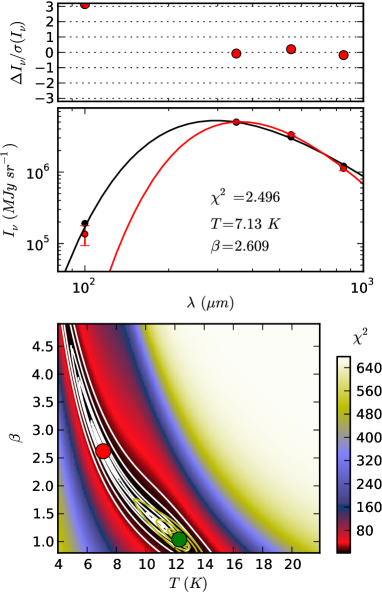
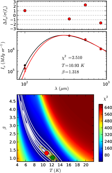
Figure 18: Another example of a case with the $\chi^{2}$ having two distinct minima in the ($T_{\rm C}$, $\beta$) plane. The jump between the two minima takes place between the cases where the original 100 $\mu$m error estimate is scaled by 0.702 (left frames) and 0.700 (right-hand frames).

Appendix B The bias and scatter of the $T_{\rm C}$ and $\beta_{\rm obs}$ values

In Sect. 3.2 we examined the appearance of multiple $\chi^{2}$ minima for modified black body spectra. The parameters $T_{\rm C}$ and $\beta_{\rm obs}$ can, of course, have bias and scatter also independent of the problem of possible double $\chi^{2}$ minima. Figures 19 and 20 show these for the tests with single modified black body spectra. The biases and the standard deviations of the colour temperature and the spectral index showed no significant dependence on the parameter $K_{\rm 100}$ and therefore the figures are drawn using only values $K_{\rm 100}$=1.0. Otherwise the figures correspond to the cases shown in Figs. 9 and 10.

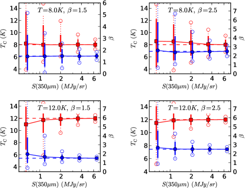
Figure 19: Distribution of $T_{\rm C}$ (red squares and left-hand axis) and $\beta_{\rm Obs}$ (blue circles and right-hand axis) for single modified black body spectra with noise and data at the wavelengths of 100, 350, 550, and 850 $\mu$m (cf. Fig. 9). The solid vertical lines connect the quartile points and the open circles corresponds to the 10% and 90% percentage points of the parameter distributions.

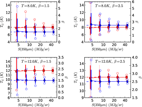
Figure 20: As Fig. 19 but for observations at the wavelengths of 100, 250, 350, and 500 $\mu$m (cf. Fig. 10).