Empirical Fit to electron-nucleus scattering.

Abstract

An empirical fit to electron-nucleus scattering for $A>2$ is made based on world data. It is valid for $0<W<3.2$ GeV and $0.2<Q^{2}<5$ GeV², and can be used with caution at lower $Q^{2}$. The fit is based on previous empirical fits to electron-proton and electron-neutron scattering, taking into account the effects of Fermi motion plus a substantial extra contribution that fills in the dip between the quasi-elastic peak and the $\Delta(1232)$ resonance.

I Introduction

There are many applications in nuclear/particle physics for a reliable parametrization of inclusive electron-nucleus scattering. One example is the reliable evaluation of radiative corrections to measured data to extract inclusive electron scattering cross sections. Another is the evaluation of background in electron scattering from polarized ammonia. In this case, the contributions from the unpolarized nitrogen relative to the polarized proton must be taken into account to extract spin-dependent inclusive cross section asymmetries.

A prime motivation for a new empirical fit is the availability of a large body of new, high precision electron-nucleus scattering data from Jefferson Lab Mamyan . The present fit was used in the evaluation of the radiative corrections for much of these data.

Our basic fit form is similar to that of a previous fit to inclusive electron-deuteron scattering Bosted .

II Definitions and Kinematics

In terms of the incident electron energy, $E$, the scattered electron energy, $E^{{}^{\prime}}$, and the scattering angle, $\theta$, the absolute value of the exchanged 4-momentum squared in electron-nucleon scattering is given by

$$Q^{2}=(-q)^{2}=4EE^{{}^{\prime}}{\sin}^{2}\frac{\theta}{2},$$ (1)

and the mass of the undetected hadronic system is

$$W^{2}=M_{p}^{2}+2M_{p}\nu-Q^{2},$$ (2)

with $M_{p}$ the proton mass, $\nu=E-E^{\prime}$, and the small terms involving the electron mass squared have been neglected.

In the one-photon exchange approximation, the spin-independent cross section for inclusive electron-nucleon scattering can be expressed in terms of the photon helicity coupling as

$$\frac{d\sigma}{d\Omega dE^{{}^{\prime}}}=\frac{\alpha_{F}^{2}\cos^{2}(\theta/2)}{[2E\sin^{2}(\theta/2)]^{2}}(W_{2}(W^{2},Q^{2})+2\tan^{2}(\theta/2)W_{1}(W^{2},Q^{2})]$$ (3)

where $\alpha_{F}=1/137$ is the fine structure constant, and the structure functions $W_{1}$ and $W_{2}$ are each the sum of a quasi-elastic ($W^{QE}$) and an inelastic $(W^{I})$ piece, as detailed below. The quasi-elastic fit is given in terms of the $F_{1}$ and $F_{2}$ structure functions, which are related to $W_{1}$ and $W_{2}$ by $F_{1}=MW_{1}$ and $F_{2}=\nu W_{2}$.

III Inelastic Fit function

The functional form of the fit is:

$$W_{1}^{I}=(W_{1}^{F}(W^{2},Q^{2})+W_{1}^{MEC}(W^{2},Q^{2}))f_{EMC}(x^{\prime})$$

where $W_{1}^{F}$ is a Fermi-smeared sum of free proton and neutron contributions, $W_{1}^{MEC}$ is an additional term to fill in the dip between quasi-elastic and $\Delta(1232)$ peaks, and $f_{EMC}$ is an unpublished parametrization of the “EMC” effect (nuclear dependence of Deep Inelastic Scattering) by S. Rock in 1994.

To obtain $W_{2}^{I}$, we use the relation:

$$W_{2}^{I}=W_{1}^{I}[1+R_{A}(W,Q^{2})]/(1+\nu^{2}/Q^{2})$$

where

$$R_{A}(W,Q^{2})=R_{p}(W,Q^{2})(1+P_{6}+P_{23}A)$$

where $R_{p}$ is the ratio of longitudinal to transverse cross sections from the fit to world proton data given in Ref. Christy . The fit parameters $P_{i}$ are listed in Table 3.

III.1 Inelastic term $W_{1}^{F}(W^{2},Q^{2})$

To obtain the inelastic term, $W_{1}^{F}(W^{2},Q^{2})$, we use the equation:

$$W_{1}^{F}(W^{2},Q^{2})=C(x)\sum_{i}[ZW_{1}^{p}((W_{i}^{\prime})^{2},Q^{2})+(A-Z)W_{1}^{n}((W_{i}^{\prime})^{2},Q^{2})]f_{i}$$ (4)

where the correction term depending on $x$ Bjorken is given by:

$$C(x)=1+P_{13}x+P_{14}x^{2}+P_{15}x^{3}+P_{16}x^{4}+P_{17}x^{5},$$ (5)

and $W_{1}^{p}$ and $W_{1}^{n}$ are the free proton Christy and neutron Bosted structure functions. The shifted values $W_{i}^{\prime}$ are given by

$$(W_{i}^{\prime})^{2}=W^{2}+\xi_{i}k_{F}|\vec{q}|-2E_{s}(\nu+M)$$ (6)

where $|\vec{q}|^{2}=Q^{2}+\nu^{2}$,

$$\xi_{i}=-3+6(i-1)/98$$ (7)

and

$$f_{i}=0.0245e^{(-\xi_{i}^{2}/2)}.$$ (8)

The sum is nothing more than a step-wise integration over a Gaussian whose width is controlled by a Fermi momentum $k_{F}$, truncated at $\pm 3\sigma$, with a shift in central $W$ related to the binding energy $E_{s}$. The values of $k_{F}$ and $E_{s}$ used for the different nuclei are given in Table 1.

$A$	$k_{F}$ (GeV)	$E_{s}$ (GeV)
3	0.115	0.001
$3<A<8$	0.190	0.017
$7<A<17$	0.228	0.0165
$16<A<26$	0.230	0.023
$25<A<39$	0.236	0.018
$38<A<56$	0.241	0.028
$55<A<61$	0.241	0.023
$A>60$	0.245	0.018

Table 1: Values of Fermi-broadening parameter $k_{F}$ and binding energy parameter $E_{s}$ for different nuclei.

III.2 “MEC” term

To fill in the dip between the quasi-elastic and $\Delta(1232)$ resonance peaks, we added an extra term, which we dubbed the “MEC” (meson-exchange current) term. The importance of this term grows with $A$. The form of $W_{1}^{MEC}$ is:

$$W_{1}^{MEC}=\frac{P_{0}}{f}e^{-[(\sqrt{W^{2}}-P_{1})^{2}]/P_{2}]}$$ (9)

where

$$f=(1+(Q^{2})^{\prime})/P_{3})^{P_{4}}\hskip 10.84006pt\nu^{P_{5}}\hskip 10.84006pt(1+P_{18}A^{(1+P_{19}x)})$$ (10)

where $(Q^{2})^{\prime})$ is the larger of 0.3 GeV² or $Q^{2}$ and $x=Q^{2}/2M\nu$.

III.3 $f_{EMC}$

The function $f_{EMC}$ is given by:

$$f_{EMC}=cA^{\alpha}$$

where

$$\alpha=\alpha_{0}+\sum_{i=1}^{8}\alpha_{i}(x^{\prime})^{i}$$

where $x^{\prime}$ is the smaller of 0.7 and $Q^{2}/2M\nu$ and the coefficients $\alpha_{i}$ are given in Table 2, and where

$$c=e^{0.0169+0.01809x^{\prime}+0.0050427(x^{\prime})^{2}}$$

The $f_{EMC}$ fit is illustrated for five representative nuclei in Fig. 1. Note that the original fit was only for data with Bjorken $x<0.7$, that is why we “freeze” the results above that value

$\alpha_{0}$	$\alpha_{1}$	$\alpha_{2}$	$\alpha_{3}$	$\alpha_{4}$	$\alpha_{5}$	$\alpha_{6}$	$\alpha_{7}$	$\alpha_{8}$
-0.069887	2.1888	-24.667	145.29	-497.23	1013.1	-1208.3	775.76	-205.87

Table 2: Values of the $\alpha_{i}$ EMC fit parameters.

Figure 1: Illustration of the $x$-dependence of the function $f_{EMC}$ for five values of atomic number A.

IV Fit parameters

The fit parameters are given in Table 3, except for $P_{18}$. This parameter, which is important in the strength of the MEC term, was fit individually for ${}^{3}He$, ${}^{4}He$, C, Al, and Cu. We assume nearby nuclei will have the same parameter values. The results are given in Table 4.

$P_{0}$	0.005138	$P_{1}$	0.980710
$P_{2}$	0.046379	$P_{3}$	1.643300
$P_{4}$	6.982600	$P_{5}$	-0.226550
$P_{6}$	0.110950	$P_{7}$	0.027945
$P_{8}$	0.406430	$P_{9}$	1.607600
$P_{10}$	-7.546000	$P_{11}$	4.441800
$P_{12}$	-0.374640	$P_{13}$	0.104140
$P_{14}$	-0.268520	$P_{15}$	0.966530
$P_{16}$	-1.905500	$P_{17}$	0.989650
$P_{18}$	see Table 2	$P_{19}$	-0.045536
$P_{20}$	0.249020	$P_{21}$	-0.137280
$P_{22}$	29.201000	$P_{23}$	0.004928

Table 3: Values of the fit parameters.

A	$P_{18}$
3	70
4	170
$4<A<21$	215
$20<A<51$	235
$A>50$	230

Table 4: Values of $P_{18}$ for different nuclei.

V Quasi-elastic contribution

The quasi-elastic contribution is calculated using the equations in Ref. Sick . The free nucleon factors are taken from Ref. FF . These form factors are based on inclusive electron scattering, and thus have the 2-photon corrections appropriate to the present quasi-elastic fit. The values of Fermi motion parameter $k_{F}$ and binding energy $E_{s}$ are slightly different than in Ref. Sick : we used those in Table 1. We used a multiplicative Pauli suppression factor given by

$$(3/4)(|\vec{q}|/k_{F})(1-(|\vec{q}|/k_{F})^{2})/12)$$

for $|\vec{q}|<2k_{F}$, otherwise no correction was made. We assumed the same suppression for $W_{1}$ and $W_{2}$. For the scaling function, we used Fy

$$F(\psi^{\prime})=1.5576/k_{F}(1+1.7720^{2}(\psi^{\prime}+0.3014)^{2})(1+e^{-2.4291\psi^{\prime}})$$ (11)

We used the same function for both $W_{1}$ and $W_{2}$.

The nominal results from the above were corrected as follows:

$$F_{1}=F_{1}^{nom}(1+P_{7}+P_{8}y+P_{9}y^{2}+P_{10}y^{3}+P_{11}y^{4})$$

and

$$R=R^{nom}(1+P_{12})$$

where $R^{nom}$ is the ratio of longitudinal to transverse cross sections, defined using:

$$R^{nom}=(F_{2}^{nom}/\nu)(M/F_{1}^{nom})(1.+\nu^{2}/Q^{2})-1$$

and where $y=(W^{2}-M^{2})/|\vec{q}|$. The fit parameters $P_{7}$ to $P_{12}$ are given in Table 3.

VI Coulomb Corrections

Coulomb corrections are taken into account in the simple energy gain/loss method, using a slightly higher incident and scattered electron energies at the vertex than measured in the lab. The shifts are the same in both cases, and are given by Coulomb :

$$V=0.775\hskip 3.61371pt\frac{3}{2}\hskip 3.61371pt\alpha_{F}(Z-1)/R_{0}$$ (12)

where $R_{0}$ (in units of GeV) is given by:

$$R_{0}=1.1A^{(1/3)}+0.86A^{(-1/3)}$$ (13)

VII Discussion

To illustrate the main features of the fit, the response function $F_{2}$ is plotted versus $W$ for He (left) and Fe (right) in Fig. 2. The top curve in each plot is the sum of the there components: a quasi-elastic peak centered on $M$, a smaller but broader “MEC” peak centered near $W=1.05$ GeV, and the inelastic continuum. The main two features that can be noticed are that the quasi-elastic and $\Delta(1232)$ peaks are wider in Fe than in He (due to the larger Fermi momentum), and the MEC contribution is relatively larger in Fe than in He.

Figure 2: Illustration of the $W$-dependence of the structure function $F_{2}(W,Q^{2})$ for He (left) and Fe (right), for $Q^{2}=0.6$ GeV². The upper curves are the sum of the three lower curves (quasi-elastic, “MEC”, and inelastic, from left to right).

The $Q^{2}$ dependence of $F_{1}$ is illustrated for C and Al in Fig. 3. Note the very prominent quasi-elastic and $\Delta(1231)$ peaks at low $Q^{2}$, which “disappear” rapidly at higher $Q^{2}$. This feature is what makes at fit accurate to better than 10% so difficult for $Q^{2}<0.2$ GeV².

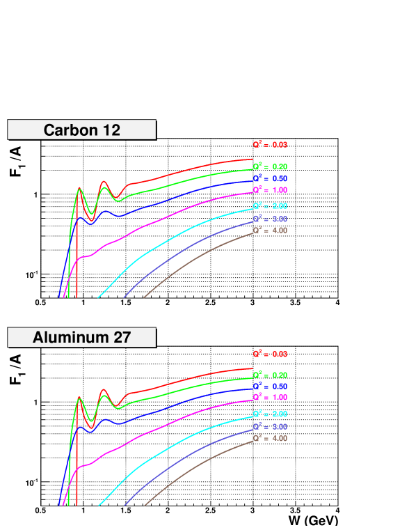
Figure 3: Illustration of the $W$-dependence of the structure function $F_{1}(W,Q^{2})$ (per nucleon) for C and Al for a wide range of $Q^{2}$ values (units are GeV²).

The fit is compared with world data Day ; Mamyan for He, C, Al, and Fe/Cu in Figs. 4-7. For $W>1.2$ GeV, the agreement is generally within 5%, and better than 3% on average. In the quasi-elastic peak region, some larger oscillations around unity can be seen due to the difficulty in matching the precise shape of the quasi-elastic peak with actual data, but on average the agreement is within 5%. The biggest discrepancies are seen at low $Q^{2}$, where the limitations of the plane-wave impulse approximation for quasi-elastic scattering become most apparent. Figure 8 shows the frequency distribution of the deviations (in percent) between data and fit for all the data points used.

Figure 4: Ratios between fit and world data for ⁴He in six $Q^{2}$ bins as a function of $W$.

Figure 5: Ratios between fit and world data for C in six $Q^{2}$ bins as a function of $W$.

Figure 6: Ratios between fit and world data for Al in six $Q^{2}$ bins as a function of $W$.

Figure 7: Ratios between fit and world data for Fe and Cu in six $Q^{2}$ bins as a function of $W$.

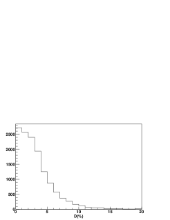
Figure 8: Frequency distribution of deviations between data and fit.

VIII Source code

The stand alone FORTRAN source code (named F1F209.f) for this fit is available Fit .

IX Acknowledgments

The authors are grateful for useful discussions with J.E. Amaro, J. Arrignton, M.B. Barbaro, M. Christy, D. Day, W.T. Donnely, and D. Gaskell.

References

- (1) V. Mamyan, Ph.D Thesis, University of Virginia, 2010. [arXiv:1202.1457].
- (2) http://faculty.virginia.edu/qes-archive/index.html
- (3) P.E. Bosted and M.E. Christy, Phys. Rev. C 77, 065206 (2008). (arXiv:0711.0159).
- (4) M.E. Christy and P.E. Bosted, accepted in Phys. Rev. C 81, 055213 (2010). (arXiv:0712.3731)
- (5) C. Maieron, T.W. Donnelly, and I. Sick, Phys. Rev. C 65, 025502 (2002).
- (6) P.E. Bosted, Phys. Rev. C 51, 409 (1995).
- (7) J.E. Amaro, M.B. Barbaro, J.A. Caballero, T.W. Donnelly, A. Molinari, and I. Sick, Phys. Rev. C 71, 015501 (2005).
- (8) A. Aste, C. von Arx, D. Trautmann, Eur. Phys. J. A26 (2005) 167.
- (9) https://userweb.jlab.org/b̃osted/fits.html