Chiral spin liquid in two-dimensional XY helimagnets

Abstract

We carry out Monte-Carlo simulations to discuss critical properties of a classical two-dimensional XY frustrated helimagnet on a square lattice. We find two successive phase transitions upon the temperature decreasing: the first one is associated with breaking of a discrete $\mathbb{Z}_{2}$ symmetry and the second one is of the Berezinskii-Kosterlitz-Thouless (BKT) type at which the $SO(2)$ symmetry breaks. Thus, a narrow region exists on the phase diagram between lines of the Ising and the BKT transitions that corresponds to a chiral spin liquid.

Pacs 64.60.De, 75.30.Kz

1. Introduction

Frustrated magnets have attracted much attention in recent years. Exotic spin liquid phases are of special interest which have been found in some of them [1]. A chiral spin liquid phase is an example of such an exotic state of matter in which there are neither quasi long-range nor long-range magnetic orders but a chiral order parameter $\langle{\bf S}_{i}\times{\bf S}_{j}\rangle$ is nonzero. Existence of such a phase is discussed in context of one-dimensional frustrated quantum magnetic systems[2], and it is found experimentally in Ref. [3].

In larger dimensions, one of the systems in which the chiral spin liquid phase can be found at finite temperature is a classical planar (XY) helimagnet with $\mathbb{Z}_{2}\otimes SO(2)$ symmetry in which the helical structure results from a competition of exchange interactions between localized spins. Critical behavior of spin systems from this class is described by two order parameters. Besides the conventional magnetization with $SO(2)$ symmetry, one has to take into account also the chiral order parameter that is an Ising variable with $\mathbb{Z}_{2}$ symmetry. This parameter characterizes the direction of the helix twist and distinguishes left-handed and right-handed helical structures.

In three-dimensional helimagnets, the phase transitions on the magnetic and the chiral order parameters occur simultaneously. It was found numerically that the transition is of the weak first order or of the ”almost second order”[4, 5] type in helical antiferromagnets on a body-centered tetragonal lattice [6] and on a simple cubic lattice with an extra competing exchange coupling along one axis [7]. These systems belong to the same (pseudo)universality class as, e.g., the model on a stacked-triangular lattice [8] and $V_{2,2}$ Stiefel model [9]. The possibility of existence and stabilization of the chiral spin liquid phase by, e.g., Dzyaloshinsky-Moria interaction in 3D helimagnets is discussed recently in Refs. [10].

In two dimensions, the situation is rather different [11]. Two successive transitions were observed with the temperature decreasing. The chiral order appears as a result of the first transition that is of the Ising type. Another one is the Berezinskii-Kosterlitz-Thouless (BKT) transition driven by the unbinding of vortex-antivortex pairs [12]. Then, the chiral spin liquid phase arises between these transitions with the chiral order and without a magnetic one. Various 2D systems from the class $\mathbb{Z}_{2}\otimes SO(2)$ were investigated numerically (see Ref. [13] for review): triangular antiferromagnet [14, 15], J₁-J₂ model [16], the Coulomb gas system of half-integer charges [17], two coupled XY models [18], Ising-XY model [19, 13, 20] and the generalized fully frustrated XY model [21]. And surely, the most famous of them is the fully frustrated XY model (FFXY) introduced by Villain [22]. This model is of great interest because it describes a superconducting array of Josephson junctions under an external transverse magnetic field [23]. It was found that the temperature of the Ising transition $T_{I}$ is $1\mbox{-}3\%$ larger than that of the BKT transition for the most of above-named systems [23, 11, 24, 13].

Korshunov argued [25] that a phase transition, driven by unbinding of kink-antikink pairs on the domain walls associated with the $\mathbb{Z}_{2}$ symmetry, can take place in models similar to 2D FFXY one at temperatures appreciably smaller than $T_{BKT}$ (see also Ref. [26]). Such a transition could lead to a decoupling of phase coherence across domain boundaries, producing in this way two separate bulk transitions with $T_{BKT}<T_{I}$ [27]. It was pointed out however in Ref. [25] that these two continuous transitions can merge into a single first order one. These conclusions do not depend on the particular form of interactions in system as soon as the ground state degeneracy remains the same. They are confirmed by numerical studies of the models mentioned above [23, 11, 24, 13, 16, 14, 15, 17].

Nevertheless the situation remains contradictory in 2D helimagnets belonging to the same $\mathbb{Z}_{2}\otimes SO(2)$ class as FFXY model and the antiferromagnet on the triangular lattice. Garel and Doniach [28] (see also [29]) considered the simplest helimagnet on a square lattice with an extra competing exchange coupling along one axis that is describing by the Hamiltonian

$$H=\sum\limits_{\mathbf{x}}\Bigl{(}J_{1}\cos(\varphi_{\mathbf{x}}-\varphi_{\mathbf{x}+\mathbf{a}})+J_{2}\cos(\varphi_{\mathbf{x}}-\varphi_{\mathbf{x}+2\mathbf{a}})-J_{b}\cos(\varphi_{\mathbf{x}}-\varphi_{\mathbf{x}+\mathbf{b}})\Bigr{)},$$ (1)

where the sum runs over sites $\mathbf{x}=(x_{a},x_{b})$ of the lattice, $\mathbf{a}=(1,0)$ and $\mathbf{b}=(0,1)$ are unit vectors of the lattice, the coupling constants $J_{1,2}$ are positive. Using arguments of Ref. [30], they concluded [28] that at low temperatures the vertices are bound by strings, which would inhibit the BKT transition and make the Ising transition occur first with the temperature increasing. Kolezhuk noticed [31] that those arguments are not valid for a helimagnet, and showed that the Ising transition temperature is larger than the BKT one at least near the Lifshitz point $J_{2}=J_{1}/4$. It was found by Monte Carlo simulations in the recent paper [32] that $T_{BKT}>T_{I}$ at $J_{2}=0.3$ and $J_{1}=J_{b}=1$ (i.e., very near the Lifshitz point) in accordance with Ref. [28] and in contrast to Ref. [31].

To account for the discordance between results for helical magnets and the general arguments for $\mathbb{Z}_{2}\otimes SO(2)$ class, we perform extensive Monte Carlo simulations of the model (1) for different values of $J_{2}$. We obtain reliable results at $J_{2}>0.4J_{1}$ which show that $T_{BKT}<T_{I}$. On the other hand the value of $T_{I}$ close to the Lifshitz point is hiding among effects of the finite size scaling and is not accessible for ordinary estimation methods. We obtain the Ising transition temperature from the chiral order parameter distribution and find that $T_{BKT}<T_{I}$ near the Lifshitz point too. At the same time we find in accordance with results of Ref. [32] that the specific heat and susceptibilities have subsidiary peaks at low $T<T_{BKT}$ near the Lifshitz point. These are anomalies which are attributed in Ref. [32] to the Ising phase transition. However, we demonstrate that these anomalies do not signify a continuous phase transition. Apparently, their origin is in metastable states which lead also to a peculiar distribution of the chiral order parameter. We find no such features in the specific heat and susceptibilities far from the Lifshitz point (at $J_{2}>0.4J_{1}$). As a result we obtain the phase diagram shown in Fig. 1.

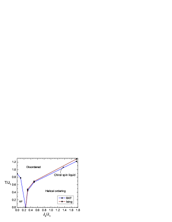
Figure 1: Phase diagram of the model (1) that is found in the present paper.

The rest of the present paper is organized as follows. We discuss in Sec. 2. the model (1) in more detail and introduce quantities to be found in our calculations. Numerical results are discussed in Sec. 3.. In particular, the Ising and the BKT transitions are considered in Secs. 3.1. and 3.2., respectively. The neighborhood of the Lifshitz point and the phase diagram are discussed in Sec. 3.3.. Sec. 4. contains our conclusions.

2. Model and methods

We consider the model (1) of the classical XY magnet on a square lattice. We set $J_{1}=J_{b}=1$ for simplicity and the value of the extra exchange interaction $J_{2}$ is a variable. The Lifshitz point corresponds to $J_{2}=1/4$ in this notation. The system has a collinear antiferromagnetic ground state at $J_{2}<1/4$. To discuss the phase transition from the (quasi-)antiferromagnetic phase to the paramagnetic one we consider $J_{2}=0$ and $J_{2}=0.1$ (see Fig. 1). The ground state has a helical ordering at $J_{2}>1/4$. The turn angle $\theta_{0}$ between two neighboring spins along $\mathbf{a}$ axis is given by $\cos\theta_{0}=-J_{1}/4J_{2}$ at zero temperature.

To discuss the number and the sequence of phase transitions from the (quasi-)helical phase to the paramagnetic one we consider $J_{2}\approx 0.309$, 0.5 and $1.76$ corresponding at $T=0$ to angles of commensurate helices $\theta_{0}=4\pi/5$, $2\pi/3$ and $6\pi/11$, respectively. We use lattices with $L^{2}$ cites, where $L$ is divisible by the size of the helix pitch and it lies in the range from 20 to 120. We apply the periodic (toric) boundary conditions as well as the cylindrical ones (i.e., with the periodic condition along the $\mathbf{b}$ axis and the free one along the $\mathbf{a}$ axis). We have found that both conditions lead to the same values of transition temperatures and indexes. In contrast values of Binder’s cumulants and the chiral order parameter distribution at $J_{2}\approx 0.309$ depend on boundary conditions as we discuss below in detail. Standard Metropolis algorithm [35] has been used. The thermalization was maintained within $4\cdot 10^{5}$ Monte Carlo steps in each simulation. Averages have been calculated within $3.6\cdot 10^{6}$ steps for ordinary points and $6\cdot 10^{6}$ for points close to the critical ones. We have used also the histogram analysis technique in which the range of each quantity has been divided into $6.4\cdot 10^{5}$ bins.

2.1. Order parameters

The BKT transition is driven by the magnetic order parameter for which we use two definitions. Similar to the triangular lattice [14], one can introduce a number of sublattices in the case of helix pitches which are divisible by the lattice constant. Then, one can write for the magnetic order parameter

$$\mathbf{m}_{i}=\frac{n_{sl}}{L^{2}}\sum_{\mathbf{x}_{i}}\mathbf{S}_{\mathbf{x}_{i}},\quad\overline{m}=\sqrt{\frac{1}{n_{sl}}\sum\limits_{i}\left<\mathbf{m}_{i}^{2}\right>},$$ (2)

where index $i$ enumerates $n_{sl}$ sublattices, the sum over $\mathbf{x}_{i}$ runs over sites of the $i$-th sublattice, spin $\mathbf{S}_{\mathbf{x}_{i}}=(\cos\phi_{\mathbf{x}_{i}},\sin\phi_{\mathbf{x}_{i}})$ is a classical two-component unit vector, and $\langle\ldots\rangle$ denotes the thermal average. The second definition of the order parameter is valid both for commensurate and incommensurate helices

$$\mathbf{M}_{j}=\frac{1}{L}\sum_{i}\mathbf{S}_{j\mathbf{a}+i\mathbf{b}},\quad\overline{M}=\sqrt{\frac{1}{L}\sum_{j}\left<\mathbf{M}_{j}^{2}\right>}.$$ (3)

Our calculations show that definitions (2) and (3) lead to the same results away from the Lifshitz point. We have found that $\bf m$ shows an anomalous behavior at $J_{2}\approx 1/4$ and we use definition (3) in this case. Thus, we demonstrate that it is useful in numerical discussion of helimagnets to choose parameters of the Hamiltonian so that the helix pitch at $T=0$ to be commensurate.

The Ising transition is driven by the chiral order parameter defined as

$$k=\frac{1}{L^{2}\sin\theta_{0}}\sum\limits_{\mathbf{x}}\sin(\varphi_{\mathbf{x}}-\varphi_{\mathbf{x}+\mathbf{a}}),\quad\overline{k}=\sqrt{\left<k^{2}\right>}.$$ (4)

2.2. Susceptibilities and cumulants

We introduce corresponding susceptibilities for all order parameters [36]

$$\chi_{p}=\left\{\begin{array}[]{ll}\displaystyle\frac{L^{2}}{T}\left(\left<p^{2}\right>-\left<|p|\right>^{2}\right),&T<T_{c},\\ &\\ \displaystyle\frac{L^{2}}{T}\left<p^{2}\right>,&T\geq T_{c}.\end{array}\right.$$ (5)

The second line in this definition is used below for estimation of critical exponents. Binder’s cumulants [36] are define as

$$U_{p}=1-\frac{\langle p^{4}\rangle}{3\langle p^{2}\rangle^{2}}.$$ (6)

We discuss also the cumulant

$$V_{k}=\frac{\partial}{\partial(1/T)}\ln\langle k^{2}\rangle=L^{2}\left(\frac{\left<k^{2}E\right>}{\left<k^{2}\right>}-\langle E\rangle\right),$$ (7)

using which the critical exponent $\nu_{k}$ can be found by finite-size scaling analysis [37].

2.3. Helicity modulus

It is useful to introduce the helicity modulus (or the spin stiffness) [38] to discuss the BKT transition that is defined by the increase in the free energy density $F$ due to a small twist $\Delta_{\mu}$ across the system in one direction ($\bf a$ or $\bf b$)

$$\Upsilon_{\mu}=\left.\frac{\partial^{2}F}{\partial{\Delta_{\mu}}^{2}}\right|_{\Delta_{\mu}=0},$$ (8)

where $\mu=a,b$ denotes the direction. Important universal properties of a BKT transition predicted by Kosterlitz and Nelson [39] are the jump of the helicity modulus (8) from zero at $T>T_{BKT}$ to the value of $2T_{BKT}/\pi$ at $T=T_{BKT}$ and the value of the exponent $\eta(T=T_{BKT})=1/4$. These properties have become standard methods of finding the transition temperature.

As a result of the fact that the exchange couplings along $\mathbf{a}$ and $\mathbf{b}$ axes are different, the helicity moduli in these directions differ too. Thus, at zero temperature $\Upsilon_{a}(0)=4J_{2}-J_{1}^{2}/(4J_{2})$, while $\Upsilon_{b}(0)=J_{b}$. Nevertheless, both $\Upsilon_{a}$ and $\Upsilon_{b}$ must vanish at the same temperature with the identical value of the jump.

One finds after trivial calculations using Eqs. (1) and (8) that the helicity modulus $\Upsilon_{b}$ is expressed via correlation functions and has a common view [40]

$$\Upsilon_{b}=\left<E^{\prime\prime}_{b}\right>-\frac{L^{2}}{T}\left<(E^{\prime}_{b})^{2}\right>,$$ (9)

where $T$ is measured in units of $J_{1}=J_{b}=1$, we set $k_{B}=1$, $E^{\prime}_{b}=L^{-2}\sum_{\mathbf{x}}\sin(\varphi_{\mathbf{x}}-\varphi_{\mathbf{x}+\mathbf{b}})$ and $E^{\prime\prime}_{b}=L^{-2}\sum_{\mathbf{x}}\cos(\varphi_{\mathbf{x}}-\varphi_{\mathbf{x}+\mathbf{b}})$. Similar calculations give for the helicity modulus in the $\mathbf{a}$ direction

$$\Upsilon_{a}=\left<E^{\prime\prime}_{a}\right>-\frac{L^{2}}{T}\left<(E^{\prime}_{a})^{2}\right>+\frac{L^{2}}{T}\left<E^{\prime}_{a}\right>^{2},$$ (10)

where $E^{\prime}_{a}=L^{-2}\sum_{\mathbf{x}}(\sin(\varphi_{\mathbf{x}}-\varphi_{\mathbf{x}+\mathbf{a}})+2J_{2}\sin(\varphi_{\mathbf{x}}-\varphi_{\mathbf{x}+2\mathbf{a}}))$ and $E^{\prime\prime}_{a}=-L^{-2}\sum_{\mathbf{x}}(\cos(\varphi_{\mathbf{x}}-\varphi_{\mathbf{x}+\mathbf{a}})+4J_{2}\cos(\varphi_{\mathbf{x}}-\varphi_{\mathbf{x}+2\mathbf{a}}))$. It may seem that the last term in Eq. (10) can be discarded as it is done with the corresponding term in Eq. (9) which is equal to zero. However it is not so because $\left<E^{\prime}_{b}\right>=0$ at all $T$ whereas $\left<E^{\prime}_{a}\right>=0$ at $T\geq T_{I}$ and $\left<E^{\prime}_{a}\right>\neq 0$ at $T<T_{I}$. To demonstrate this let us apply an infinitesimal twist $\Delta_{a}$ across the system in the $\bf a$ direction, i.e., let us replace in Eq. (1) $\varphi_{\mathbf{x}}-\varphi_{\mathbf{x}+\mathbf{a}}$ by $\varphi_{\mathbf{x}}-\varphi_{\mathbf{x}+\mathbf{a}}+\Delta_{a}$. One writes in the first order in $\Delta_{a}$

$$\sum_{\bf x}\Bigl{(}\cos(\varphi_{\mathbf{x}}-\varphi_{\mathbf{x}+\mathbf{a}}+\Delta_{a})+J_{2}\cos(\varphi_{\mathbf{x}}-\varphi_{\mathbf{x}+2\mathbf{a}}+2\Delta_{a})\Bigr{)}$$

$$\approx\sum_{\bf x}\Bigl{(}\cos(\varphi_{\mathbf{x}}-\varphi_{\mathbf{x}+\mathbf{a}})+J_{2}\cos(\varphi_{\mathbf{x}}-\varphi_{\mathbf{x}+2\mathbf{a}})\Bigr{)}$$

$$-\Delta_{a}\sum_{\bf x}\Bigl{(}\sin(\varphi_{\mathbf{x}}-\varphi_{\mathbf{x}+\mathbf{a}})+2J_{2}\sin(\varphi_{\mathbf{x}}-\varphi_{\mathbf{x}+2\mathbf{a}})\Bigr{)}.$$ (11)

Comparing the last term in Eq. (11) with the chiral order parameter $k$ definition (4) and noting that one can use an equivalent definition $\tilde{k}=L^{-2}\sum_{\mathbf{x}}\sin(\varphi_{\mathbf{x}}-\varphi_{\mathbf{x}+2\mathbf{a}})$ we conclude that the last term in Eq. (11) is a linear combination of $k$ and $\tilde{k}$. However, $k$ and $\tilde{k}$ have opposite signs in the case considered. In particular, their combination $k+2J_{2}\tilde{k}$ in the last term in Eq. (11) is equal to zero at $T=0$. Nevertheless our numerical results presented below show that this combination is not equal to zero at $T\neq 0$ and it can be considered as the Ising order parameter at $T\sim T_{I}$. Then, one see from Eq. (11) that $\Delta_{a}$ plays the role of the ”chiral” field and, consequently, $\partial F/\partial\Delta_{a}|_{\Delta_{a}=0}$ (that is equal in our notation to $\left<E^{\prime}_{a}\right>$) is proportional to the chiral order parameter which is equal to zero at $T\geq T_{I}$ and which is finite at $T<T_{I}$.

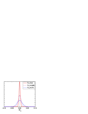
Figure 2: Distribution of the value $E_{b}^{\prime}$ defined in Eq. (9) for $J_{2}=0.5$, $L=$ and three $T$ values: $T>T_{I}$, $T<T_{BKT}$, and $T_{BKT}<T<T_{I}$.

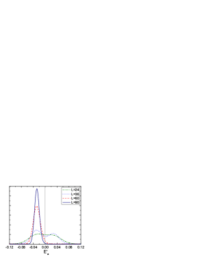
Figure 3: Distribution of the value $E_{a}^{\prime}$ defined in Eq. (10) for $J_{2}=0.5$, $T=0.67<T_{I}$ and different $L$.

To illustrate this consideration we present in Fig. 3 the distribution of $E^{\prime}_{b}$ for $J_{2}=0.5$ and for various temperatures below $T_{BKT}\approx 0.671$, between $T_{BKT}$ and $T_{I}\approx 0.69$, and above $T_{I}$ (the values of $T_{I}$ and $T_{BKT}$ are obtained below). The distribution has a Gaussian form with the zero expected value $\langle E^{\prime}_{b}\rangle=0$. Fig. 3 shows the distribution of $E^{\prime}_{a}$ for $T=0.67<T_{I}$ and various lattice sizes. A non-zero expected value of $\langle E^{\prime}_{a}\rangle$ is seen. One can observe a double-peak structure of $E^{\prime}_{a}$ distribution (see Fig. 3) for small lattices or at $T$ that is close enough to $T_{I}$, when the system can tunnel to a configuration with opposite chirality. The probability of such tunneling is estimated as

$$p(\overline{k}_{+}\to\overline{k}_{-})=\exp\left(-\frac{2Lf_{dw}}{T}\right),$$ (12)

where $f_{dw}$ is a domain wall tension [41] that is positive at $T<T_{I}$ and it vanishes at $T=T_{I}$. That is why we observe two peaks for small lattices and only one peak for large ones. Quite expectedly, we find the single-peak distribution of $E^{\prime}_{a}$ at $T>T_{I}$ demonstrated in Fig. 4.

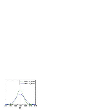
Figure 4: Same as in Fig. 3 for $T>T_{I}$.

It should be stressed that the disappearance of the double-peak structure at the critical temperature $T_{I}(L)$ is a signature of the transition on a lattice with size $L$. The value of $T_{I}(L)$ is close to the correct value of the transition temperature for large lattices. We use this circumstance below in our analysis of the Lifshitz point neighborhood.

It should be noted also that we replace in our numerical calculations $\left<E^{\prime}_{a}\right>$ by $\left<|E^{\prime}_{a}|\right>$ at $T<T_{I}$ in the last term in Eq. (10) as it is usually done in considerations of order parameters [36]. It is done because the order parameter distribution has tails in both positive and negative regions even below the transition temperature. The value $\left<p\right>$ is replaced by $\left<|p|\right>$ in Eq. (5) by the same reason.

3. Numerical results

We discuss in this section in detail our results for the special case of $J_{2}=0.5$ that corresponds at $T=0$ to 120^∘ helical structure with three sublattices. Then, we discuss the phase diagram. We consider lattices with $L=24$, 30, 36, 42, 48, 60, 72, 90, 120. The lattice with $L=18$ is also used for estimation of some quantities.

3.1. Ising transition

To obtain the Ising transition temperature $T_{I}$ we use the Binder cumulant crossing method [36]. We find for $L=24$ and 30 the temperature $T_{L^{\prime}}$ as a function of $\ln^{-1}\left(L^{\prime}/L\right)$ at which curves $U_{k}(L)$ intersect for different lattice sizes $L^{\prime}>L$. Extrapolation to the thermodynamic limit $L^{\prime}\to\infty$ gives the following transition temperature (see Figs. 6 and 6)

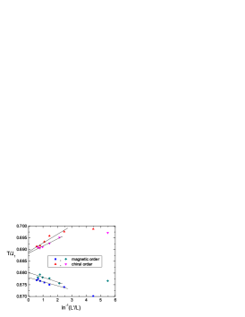
Figure 5: Estimation of the transitions temperature by the Binder cumulant crossing method.

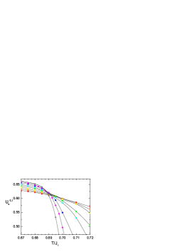
Figure 6: Binder’s cumulant $U_{k}(L)$ defined by Eq. (6) as a function of temperature, for $L=24,\ldots,90$.

$$T_{I}=0.689(1).$$ (13)

The dispersion in the value of $T_{I}$ obtained for the different lattice sizes $L$ gives the error of the transition temperature estimation. Notice that error bars are not shown in Figs. 6 and 6 and in all figures below if they are smaller than or comparable with symbols size.

A peak in the specific heat shown in Fig. 8 is found approximately at the same temperature. For the largest lattices the peak is located in the range of temperature from $0.690$ to $0.695$. One expects that this peak corresponds to the logarithmic divergence of the specific heat that is a characteristic of the 2D Ising model in which the critical exponent $\alpha$ is equal to zero. Insufficient accuracy of our data for the specific heat prevents us from the immediate estimation of $\alpha$.

Critical exponents $\nu_{k}$, $\beta_{k}$ and $\gamma_{k}$ are obtained by the finite-size scaling theory. To estimate the exponent $\nu_{k}$, we find a maximum of the quantity $V_{k}$ given by Eq. (7) as a function of lattice size $L$ [37]

$$\left(V_{k}^{(L)}\right)_{\mbox{\scriptsize max}}\sim L^{1/\nu_{k}}.$$ (14)

The fitting presented in Fig. 8 gives

$$\nu_{k}=0.97(4)$$ (15)

that coincides within the computational error with the exact value of $\nu=1$ for the 2D Ising model.

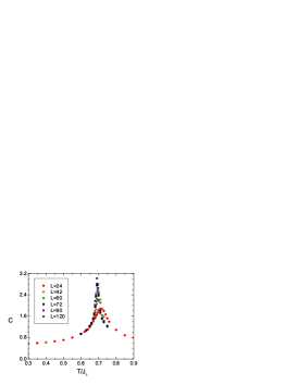
Figure 7: Specific heat $C(T)$.

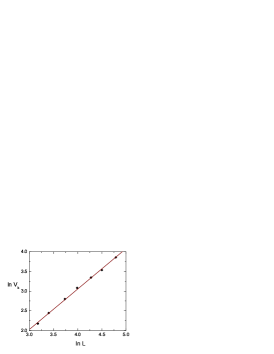
Figure 8: Estimation of the exponent $\nu_{k}$ using the cumulant $V_{k}$ defined by Eq. (7).

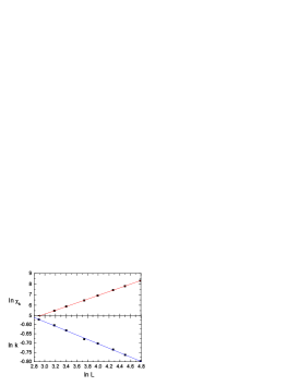
Figure 9: Estimation of the exponents $\beta_{k}$ and $\gamma_{k}$.

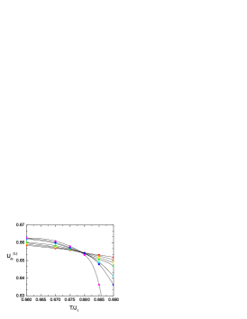
Figure 10: Binder’s cumulant $U_{m}(L)$ as a function of temperature, for $L=24,\ldots,90$.

Exponents $\beta_{k}$ and $\gamma_{k}$ are found from scaling properties of the order parameter $\overline{k}$ and the susceptibility $\chi_{k}$ at the critical point

$$\left(\bar{k}^{(L)}\right)_{T=T_{I}}\sim L^{\beta_{k}/\nu_{k}},\quad\left(\chi_{k}^{(L)}\right)_{T=T_{I}}\sim L^{\gamma_{k}/\nu_{k}},$$ (16)

with the following result (see Fig. 10):

$$\beta_{k}=0.118(8),\quad\gamma_{k}=1.70(6).$$ (17)

These values coincide within computational errors with exact values of $1/8$ and $7/4$, correspondingly, of the 2D Ising model. Using the scaling relations we find other exponents

$$\alpha=2-2\nu_{k}=0.06(8),\quad\eta_{k}=2-\gamma_{k}/\nu_{k}=0.25(5).$$ (18)

Note that the scaling relation $\alpha+2\beta_{k}+\gamma_{k}=2.00(8)\approx 2$ is satisfied within the computational error.

We have found also the universal value of the Binder cumulant $U^{*}=0.615(6)$ at the critical temperature (see Fig. 6) that is in agreement with the value $U^{*}\approx 0.611$ observed in the 2D Ising model [42] with periodic boundary conditions.

3.2. BKT transition

According to the Mermin-Wagner theorem [43] there is no spontaneous magnetization at finite temperature in 2D magnets with short range interactions and a continuous symmetry. But a quasi-long-range order appears at non-zero temperature due to the Berezinskii-Kosterlitz-Thouless mechanism [12] in XY magnets with $SO(2)$ symmetry.

It is important that as long as we measure the temperature in units of $J_{1}$, the universal value of the jump $2T_{BKT}/\pi$ perturbs by the factor of $J_{1}/J_{\mathrm{eff}}$, where $J_{\mathrm{eff}}$ is an effective coupling constant. The competing exchange coupling $J_{2}$ gives rise to this factor. To obtain it we considered the Coloumb-gas representation of the model (1) using standard duality transformations [12, 44]. As a result we obtain

$$J_{\mathrm{eff}}=\sqrt{J_{b}\left(J_{1}-4J_{2}\right)}$$ (19)

for the antiferromagnetic phase ($J_{2}<J_{1}/4$), and

$$J_{\mathrm{eff}}=\sqrt{\frac{1}{2}J_{b}\left(4J_{2}-\frac{J_{1}^{2}}{4J_{2}}\right)}$$ (20)

for the helimagnetic one ($J_{2}>J_{1}/4$). Eq. (19) is in accordance with results of Refs. [28, 45]. In particular, $J_{\mathrm{eff}}=\sqrt{3}/2$ for $J_{2}=0.5$.

A few authors have investigated the properties of the Binder cumulant for magnetization as an alternative method of the BKT transition temperature estimation [46]. Due to finite-size corrections this method gives a value for the transition temperature $T_{B}$ that is slightly larger than the true value $T_{BKT}$. Nevertheless this method is useful as it provides an estimation of the BKT transition temperature and an extra evidence of separated transitions (if one finds that $T_{B}<T_{I}$). Using the Binder cumulant crossing method described above we find $T_{B}=0.679(2)$ (see Figs. 6 and 10) that is $1.8\%$ smaller than $T_{I}$ given by Eq. (13).

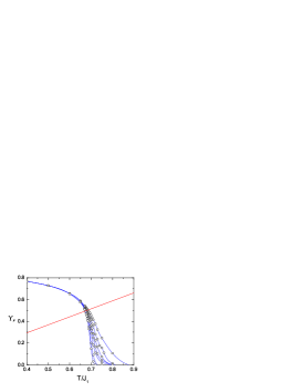
Figure 11: Helicity modulus $\Upsilon_{b}$ in the $\mathbf{b}$ direction and its intersection with the line $2T/\pi J_{\mathrm{eff}}$.

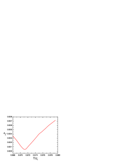
Figure 12: Root-mean-square fit error $\Delta_{c}$ of the helicity modulus $\Upsilon_{b}$ to the Weber-Minnhagen scaling equation (21).

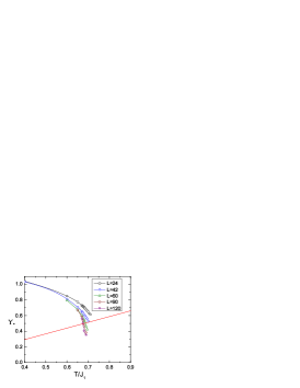
Figure 13: Same as in Fig. 12 for $\Upsilon_{a}$.

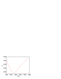
Figure 14: Same as in Fig. 12 for $\Upsilon_{a}$.

To obtain $T_{BKT}$ precisely we use the Weber-Minnhagen finite-size-scaling analysis [47] that is based on consideration of logarithmic corrections to the value of the helicity modulus at temperature close to $T_{BKT}$ having the form

$$\Upsilon(T,L)=\frac{2T}{\pi J_{\mathrm{eff}}}\left(1+\frac{1}{2\ln L+c}\right),$$ (21)

where $c$ is a fitting parameter. Fixing $T$ we find the root-mean-square error $\Delta_{c}$ of the least-square fit of our numerical data for $\Upsilon(T,L)$ with different $L\leq 60$ that is based on Eq. (21). The minimum of $\Delta_{c}$ as a function of $T$ gives the value of the transition temperature [47]. We obtain for the helicity modulus in the $\bf b$ direction (see Figs. 12 and 12)

$$T_{BKT}^{(\Upsilon_{b})}=0.671(1).$$ (22)

Corresponding results for $\Upsilon_{a}$ are shown in Figs. 14 and 14. For the largest lattice of $L\geq 48$ the Weber-Minnhagen finite-size scaling analysis estimates the BKT transition temperature as

$$T_{BKT}^{(\Upsilon_{a})}=0.673(2)$$ (23)

that is in agreement with Eq. (22). It should be noted that inaccuracy in estimation of $\Upsilon_{a}$ is larger than of $\Upsilon_{b}$. That is why we use below the more precise value (22) for comparison between different methods.

To verify our results, we use also cylindric boundary conditions with the periodic condition along the $\mathbf{b}$ axis and with the free one along the $\mathbf{a}$ axis. We obtain results consistent with those for periodic conditions. In particular, transitions temperatures $T_{BKT}=0.671(2)$ and $T_{I}=0.6907(6)$ were estimated by the Weber-Minnhagen analysis and the Binder cumulant crossing method (see Fig. 16). The universal value of the Binder cumulant at the critical temperature is $U^{*}=0.496(7)$ that is close to the value expected for the 2D Ising model [42] with mixed (cylindric) boundary conditions.

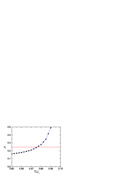
Figure 15: Intersection of the exponent $\eta(T)$ with the bound $\eta=0.25$.

Figure 16: Same as in Fig. 6 for cylindric boundary conditions.

Another indication of the BKT transition is the equality to $0.25$ of the exponent $\eta(T)$. Below the transition temperature the susceptibility diverges with the size of the system as

$$\chi_{m}(T,L)\sim L^{2-\eta(T)}.$$ (24)

The exponent $\eta$ as a function of temperature found using Eq. (24) is shown in Fig. 16. The intersection of $\eta(T)$ with the bound $\eta=0.25$ gives

$$T_{BKT}^{(\eta)}=0.676(2).$$ (25)

Comparing Eqs. (22) and (25) one notes that $T_{BKT}^{(\eta)}>T_{BKT}^{(\Upsilon)}$. Because [39] $\eta(T_{BKT})=$ $T_{BKT}J_{\mathrm{eff}}/2\pi J_{1}\Upsilon(T_{BKT})$, we can not exclude that at the true transition temperature the exponent $\eta$ and the jump of the helicity modulus have non-universal values. Such a possibility has been considered for other models from the class $\mathbb{Z}_{2}\otimes SO(2)$. [23, 24, 14, 17, 48] If it is so $\eta$ has a value smaller than 0.25 and the jump is greater than $2J_{1}/\pi J_{\mathrm{eff}}$. Thus, our data show that $\eta(T_{BKT}^{(\Upsilon)})\approx 0.22$.

3.3. Neighborhood of the Lifshitz point and the phase diagram

Besides the case of $J_{2}=0.5$ considered above in detail we have carried out similar discussions of $J_{2}=0$, 0.1, 0.309 and 1.76 to obtain the phase diagram shown in Fig. 1. Some results of this consideration are summarized in Table 1. The case of $J_{2}=0$ corresponds to the well known XY model on a square lattice and we find $T_{BKT}=0.891(2)$ that is consistent with the previous results [49].

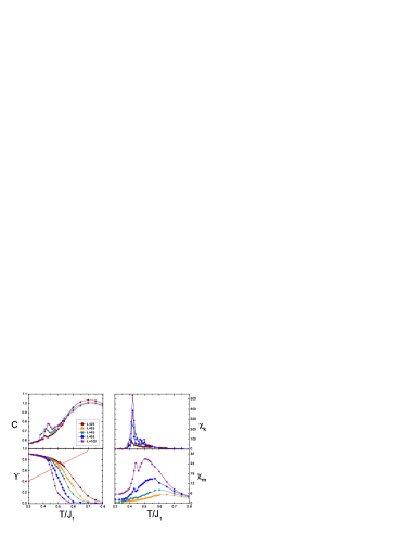
Figure 17: Specific heat $C(T)$, helicity modulus $\Upsilon_{b}$ and susceptibilities $\chi_{k,m}$ for $J_{2}\approx 0.309$.

It should be stressed that we obtain $T_{I}>T_{BKT}$ at $J_{2}>1/4$ in accordance with conclusions of Refs. [25, 31] and in contrast to Refs. [28, 32]. Because this our finding is at odds with that of the similar numerical consideration of the same model carried out in Ref. [32], our special interest is to consider the case of $J_{2}\approx 0.309$ that is close to $J_{2}=0.3$ discussed in Ref. [32].

Table 1: Some results of our discussion of the model (1). Here $L_{max}$ is the maximum value of $L$ considered.

$J_{2}/J_{1}$	$\theta_{0}$	$L_{max}$	$T_{BKT}/J_{1}$	$T_{I}/J_{1}$
$0$	0	40	0.891(2)	-
$0.1$	0	30	0.781(3)	-
$\approx 0.309$	$4\pi/5$	100	0.443(5)	0.48(1)
0.5	$2\pi/3$	150	0.671(1)	0.690(1)
$\approx 1.76$	$6\pi/11$	66	1.24(1)	1.285(7)

The case of $J_{2}\approx 0.309$ corresponds at $T=0$ to $\theta_{0}=4\pi/5$. In particular, we find $T_{BKT}=0.443(5)$ that is very close to the value reported in Ref. [32]. Estimating the temperature of the Ising critical point by the Binder cumulant crossing method, we encounter the anomalous behavior of the chiral order parameter and do not obtain a reliable result. Apparently, it is the reason why the authors of Ref. [32] base their conclusion about the Ising transition on the behavior of the specific heat $C(T)$ and susceptibilities $\chi_{k,m}$. Our results for these quantities are shown in Fig. 17 and they are consistent with those of Ref. [32]. It is seen from Fig. 17 that the chiral susceptibility has a high peak at $T\approx 0.4$, while the specific heat and the magnetic susceptibility have subsidiary peaks at $T\approx 0.4$ which grow with the lattice size increasing. These anomalies at $T\approx 0.4<T_{BKT}$ are attributed in Ref. [32] to the Ising transition.

However, we observe that for other $J_{2}>1/4$ the specific heat has only one peak corresponding to the logarithmic divergence which characterizes the Ising transition (see, e.g., Fig. 8 for $J_{2}=0.5$). Therefore, the behavior of $C(T)$ shown in Fig. 17 is not normal for the model discussed and it is characteristic of the Lifshitz point neighborhood. To account for this anomaly we examine the behavior of the chiral order parameter in detail.

Fig. 19 shows the chiral order parameter distribution for $J_{2}=0.5$ and $L=45$. It looks like a customary order parameter distribution in a system with the second order transition. In particular, the distribution has a Gaussian form below a critical temperature with a peak at $\bar{k}$ (see the curve for $T=0.6$). In approaching to the critical temperature the distribution acquires an appreciable tail (see curves for $T=0.68$ and $T=0.7$). Such a broad distribution leads to a peak in the susceptibility. The distribution has a peak at $k=0$ above the critical point (see curves for $T=0.72$ and $T=0.8$).

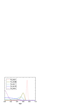
Figure 18: The chiral order parameter distribution for $J_{2}=0.5$ and $L=42$.

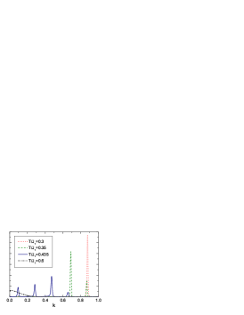
Figure 19: The chiral order parameter distribution for $J_{2}=0.309$, $L=45$ at different temperatures.

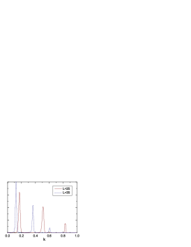
Figure 20: The chiral order parameter distribution for $J_{2}=0.309$, $L=25$ and $L=35$ at $T/J_{1}=0.43$.

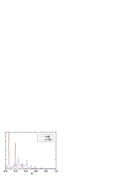
Figure 21: The chiral order parameter distribution for $J_{2}=0.309$, $L=65$ and $L=100$ at $T/J_{1}=0.43$.

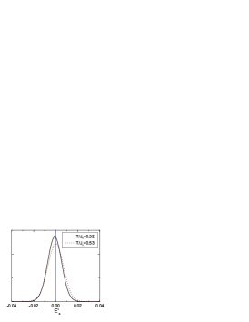
Figure 22: Distribution of $E_{a}^{\prime}$ defined in Eq. (10) for $L=65$.

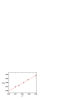
Figure 23: Estimation of $T_{I}$ for $J_{2}=0.309$ that is based on Eq. (26).

However the picture for the chiral order parameter distribution is quite different close to the Lifshitz point, e.g., at $J_{2}\approx 0.309$. We show in Fig. 19 the chiral order parameter distribution for $L=45$ and different temperatures. One can see one Gaussian peak at $T<0.35$ in agreement with the common picture described above. But a few additional peaks arise at $T>0.35$. Then, the number and the breadth of peaks depend on the lattice size $L$ (see Figs. 21 and 21) and, what is much more important, on the boundary conditions. For the cylindrical boundary conditions, these peaks are broader and they are accompanied by great number of accessory peaks. Such a distribution of the chiral order parameter is characteristic in the case of $L=45$ to the range of temperature from $T\approx 0.35$ to $T\approx 0.55$. One can see from Fig. 19 that at $T=0.57$ the distribution has a form that is typical for a disordered phase with the peak at zero value of the order parameter. Then, it is clear that the order parameter distribution at $T\approx 0.4$ shown in Fig. 19 does not correspond to a critical point of a continuous transition.

Apparently, the origin of such a peculiar behavior at $J_{2}\approx 0.309$ are metastable states with different values of the chiral order parameter which prevent the system investigation considerably. The multi-peak structure of the order parameter distribution leads to a sudden jump of the susceptibility and states intermediate between metastable configurations give rise to the specific heat anomaly. It should be noted that energy values of the metastable states are close since we observe in our simulations that the energy distribution has a Gaussian form even for the largest lattice size.

To estimate the Ising transition temperature at $J_{2}\approx 0.309$ we analyze $E^{\prime}_{a}$ distribution defined in Eq. (10) and discussed in Sec. 2.3.. As it is pointed out above, $\langle E^{\prime}_{a}\rangle\neq 0$ whenever a helical ordering exists. Fig. 23 shows that the distribution is not symmetric relative to zero at $T=0.52$ and $L=65$, while it is definitely symmetric at $T\geq 0.53$. Therefore, the critical temperature for $L=65$ can be roughly estimated as $T_{I}(L)=0.53(1)$. The transition temperature can be estimated using the relation

$$T_{I}=T_{I}(L)-\frac{A}{L^{\nu}},$$ (26)

where $A$ is constant and $\nu=1$ as it is expected for an Ising transition. An extrapolation to the thermodynamic limit using Eq. (26) gives $T_{I}=0.477(12)$ (see Fig. 23). Then, we obtain that $T_{BKT}<T_{I}$ even in the neighborhood of the Lifshitz point.

4. Conclusion

We discuss critical properties of the 2D helimagnet described by the Hamiltonian (1). It belongs at $J_{2}/J_{1}>1/4$ to the same class universality as the fully frustrated XY model and the antiferromagnet on triangular lattice which have two successive phase transitions upon the temperature decreasing: the first one is associated with breaking of the discrete $\mathbb{Z}_{2}$ symmetry and the second one is of the BKT type at which the $SO(2)$ symmetry breaks. We confirm that this scenario is realized also in the model (1) at $J_{2}/J_{1}>1/4$ and obtain the phase diagram shown in Fig. 1. A narrow region exists on this phase diagram between lines of the Ising and the BKT transitions that corresponds to the chiral spin liquid.

In particular, we demonstrate that the number and sequence of transitions do not depend on the turn angle $\theta_{0}$ of the helix twist at $T=0$. Then, this quantity is not a critical parameter that has been already found [6, 50] in three-dimensional helimagnets. We find that it is useful in numerical discussion of helimagnets to choose parameters of the Hamiltonian so that the helix pitch at $T=0$ to be commensurate. It allows to use definition (2) of the magnetic order parameter in which the summation over sublattices is involved.

We find in accordance with results of Ref. [32] that the specific heat and susceptibilities have subsidiary peaks at low $T$ near the Lifshitz point $J_{2}/J_{1}=1/4$ (see Fig. 17). However, in contrast to the conclusion of Ref. [32] we demonstrate that these anomalies do not signify a continuous phase transition. Apparently, their origin is in metastable states near the Lifshitz point which lead also to a peculiar distribution of the chiral order parameter shown in Fig. 19.

This work was supported by the RF President (grant MD-274.2012.2), the RFBR grant 12-02-01234, and the Program ”Neutron Research of Solids”.

References:

- [1] L. Balents, Nature 464, 199 (2010).
- [2] T. Hikihara et al., Phys. Rev. B 78, 144404 (2008); J. Sudan, A. Lüscher, and A.M. Läuchli, Phys. Rev. B 80, 140402 (2009); S. Furukawa, M. Sato, and S. Onoda, Phys. Rev. Lett. 105, 257205 (2010).
- [3] F. Cinti et al., Phys. Rev. Lett. 100, 057203 (2008).
- [4] G. Zumbach, Phys. Rev. Lett. 71, 2421 (1993); Nucl. Phys. B 413, 771 (1994); Phys. Lett. A 190, 225 (1994).
- [5] B. Delamotte, D. Mouhanna, and M. Tissier, Phys. Rev. Lett. 84, 5208 (2000); Phys. Rev. B 67, 134422 (2003); 69, 134413 (2004).
- [6] H.T. Diep, Phys. Rev. B 39, 397 (1989); D. Loison, Physica A 275, 207 (2000).
- [7] A.O. Sorokin and A.V. Syromyatnikov, JETP 112, 1004 (2011); 113, 673 (2011).
- [8] H. Kawamura, J. Phys.: Cond. Mat. 10, 4707 (1998).
- [9] H. Kunz and G. Zumbach, J. Phys. A: Math. Gen. 26, 3121 (1993); D. Loison and K.D. Schotte, Eur. Phys. J. B 5, 735 (1998).
- [10] S. Onoda and N. Nagaosa, Phys. Rev. Lett. 99, 027206 (2007); F. David and T. Jolicœur, Phys. Rev. Lett. 76, 3148 (1996); N. Nagaosa, J. Phys.: Conds. Mat. 20, 434207 (2008); T. Okubo and H. Kawamura, Phys. Rev. B 82, 014404 (2010).
- [11] P. Olsson, Phys. Rev. Lett. 75, 2758 (1995); Phys. Rev. B 55, 3585 (1997).
- [12] V.L. Berezinskii, Sov. Phys. JETP 32, 493 (1971); 34, 610 (1972); J.M. Kosterlitz and D.J. Thouless, J. Phys. C: Solid State Phys. 6, 1181 (1973); J.M. Kosterlitz, J. Phys. C: Solid State Phys. 7, 1046 (1974).
- [13] M. Hasenbusch, A. Pelissetto, and E. Vicari, J. Stat. Mech., P12002 (2005).
- [14] S. Miyashita and J. Shiba, J. Phys. Soc. Jpn. 53, 1145 (1984); D.H. Lee et al., Phys. Rev. Lett. 52, 433 (1984); Phys. Rev. B 33, 450 (1986); W.Y. Shih and D. Stroud, Phys. Rev. B 30, 6774 (1984); H.-J. Xu and B.W. Southern, J. Phys. A: Math. Gen. 29, L133 (1996); S. Lee and K.-C. Lee, Phys. Rev. B 57, 8472 (1998).
- [15] J.-H. Park et al., Phys. Rev. Lett. 101, 167202 (2008).
- [16] P. Simon, J. Phys A: Math. Gen. 30, 2653 (1997); Europhys. Lett. 39, 129 (1997); D. Loison and P. Simon, Phys. Rev. B 61, 6114 (2000).
- [17] J.M. Thijssen and H.J.F. Knops, Phys. Rev. B 37, 7738 (1988); G.S. Grest, Phys. Rev. B 39, 9267 (1989); J.-R. Lee, Phys. Rev. B 49, 3317 (1994).
- [18] N. Parga and J.E. Van Himbergen, Solid State Commun. 35, 607 (1980); M.Y. Choi and S. Doniach, Phys. Rev. B 31, 4516 (1985); M. Yosefin and E. Domany, Phys. Rev. B 32, 1778 (1985); M.Y. Choi and D. Stroud, Phys. Rev. B 32, 5773 (1985); E. Granato and J.M. Kosterlitz, Phys. Rev. B 33, 4767 (1986); J. Appl. Phys. 64, 5636 (1988).
- [19] S.E. Korshunov, JETP Lett. 41, 263 (1985); E. Granato, J. Phys. C: Solid State Phys. 20, L215 (1987); E. Granato et al., Phys. Rev. Lett. 66, 1090 (1991); J. Lee, E. Granato, and J.M. Kosterlitz, Phys. Rev. B 43, 11531 (1991); 44, 4819 (1991); M.P. Nightingale, E. Granato, and J.M. Kosterlitz, Phys. Rev. B 52, 7402 (1995); S. Lee, K.-C. Lee, and J.M. Kosterlitz, Phys. Rev. B 56, 340 (1997); M. Hasenbusch, A. Pelissetto, and E. Vicari, Phys. Rev. B 72, 184502 (2005).
- [20] O. Foda, Nucl. Phys. B 300, 611 (1988); P. Baseilhac, Nucl. Phys. B 636, 465 (2002); G. Cristofano et al., J. Stat. Mech., P11009 (2006).
- [21] E. Domany, M. Schick, and R.H Swendsen, Phys. Rev. Lett. 52, 1535 (1984); A. Jonsson and P. Minnhagen, Phys. Rev. Lett. 73, 3576 (1994); P. Minnhagen et al., Phys. Rev. B 76, 224403 (2007).
- [22] J. Villain, J. Phys. C: Solid State Phys. 10, 1717 (1977); 10, 4793 (1977).
- [23] S. Teitel and C. Jayaprakash, Phys. Rev. B 27, 598 (1983); Phys. Rev. Lett. 51, 1999 (1983).
- [24] S. Lee and K.-C. Lee, Phys. Rev. B 49, 15184 (1994); V. Cataudella and M. Nicodemi, Physica A 233, 293 (1996); G.S. Jeon, S.Y. Park, and M.Y. Choi, Phys. Rev. B 55, 14088 (1997); Y. Ozeki and N. Ito, Phys. Rev. B 68, 054414 (2003).
- [25] S.E. Korshunov, Phys. Rev. Lett. 88, 167007 (2002); Phys. Usp. 49, 225 (2006).
- [26] J.-R. Lee et al., Phys. Rev. Lett. 79, 2172 (1997); P. Olsson and S. Teitel, Phys. Rev. B 71, 104423 (2005).
- [27] T.C. Halsey, J. Phys. C: Solid State Phys. 18, 2437 (1985); S.E. Korshunov and G.V. Uimin, J. Stat. Phys. 43, 1 (1986); S.E. Korshunov, J. Stat. Phys. 43, 17 (1986).
- [28] T. Garel and S. Doniach, J. Phys. C: Solid State Phys. 13, L887 (1980).
- [29] Y. Okwamoto, J. Phys. Soc. Jpn 53, 2613 (1984).
- [30] M.B. Einhorn, R. Savit, and E. Rabinovoci, Nucl. Phys. B 170, 16 (1980).
- [31] A.K. Kolezhuk, Phys. Rev. B 62, R6057 (2000). See also numerical results T. Hikihara, M. Kaburagi, and H. Kawamura, Phys. Rev. B 63, 174430 (2001).
- [32] F. Cinti, A. Cuccoli, and A. Rettori, Phys. Rev. B 83, 174415 (2011).
- [33] G. Franzese et al., Phys. Rev. B 62, R9287 (2000).
- [34] F. Cinti, A. Rettori, and A. Cuccoli, Phys. Rev. B 81, 134415 (2010).
- [35] N. Metropolis et al., J. Chem. Phys. 21, 1087 (1953).
- [36] K. Binder, Z. Phys. B 43, 119 (1981); Phys. Rev. Lett. 47, 693 (1981).
- [37] A.M. Ferrenberg and D.P. Landau, Phys. Rev. B 44, 5081 (1991).
- [38] M.E. Fisher, M.N. Barber, and D. Jasnow, Phys. Rev. A 8, 1111 (1973).
- [39] D.R. Nelson and J.M. Kosterlitz, Phys. Rev. Lett. 39, 1201 (1977).
- [40] T. Ohta and D. Jasnow, Phys. Rev. B 20, 139 (1979).
- [41] K. Binder, Phys. Rev. A 25, 1699 (1982).
- [42] G. Kamieniarz and H.W.J. Blöte, J. Phys. A: Math. Gen. 26, 201 (1993); W. Selke, Eur. Phys. J. B 51, 223 (2006).
- [43] N.D. Mermin and H. Wagner, Phys. Rev. Lett. 17, 1133 (1966); P.C. Hohenberg, Phys. Rev. 158, 383 (1967); S. Coleman, Commun. Math. Phys. 31, 259 (1973).
- [44] V.N. Popov, Sov. Phys. JETP 37, 341 (1973); J. Villain, J. Phys. (Paris) 36, 581 (1975); J.V. Jose et al., Phys. Rev. B 16, 1217 (1977); L.P. Kadanoff, J. Phys. A: Math. Gen. 11, 1399 (1978); R. Savit, Phys. Rev. B 17, 1340 (1978); Rev. Mod. Phys. 52, 453 (1980).
- [45] T.A. Kaplan, Phys. Rev. Lett. 44, 760 (1980).
- [46] D. Loison, J. Phys.: Cond. Mat. 11, L401 (1999); M. Hasenbusch, J. Stat. Mech., P08003 (2008).
- [47] H. Weber and P. Minnhagen, Phys. Rev. B 37, 5986 (1988).
- [48] P. Minnhagen, Phys. Rev. Lett. 54, 2351 (1985).
- [49] U. Wolff, Nucl. Phys. B 322, 759 (1989); R. Gupta and C.F. Baillie, Phys. Rev. B 45, 2883 (1992); M. Hasenbusch, J. Phys. A: Math. Gen. 38, 5869 (2005).
- [50] H. Kawamura, Prog. Theor. Phys. Suppl. 101, 545 (1990).