Non-Markovian dynamics and noise characteristics in continuous measurement of a solid–state charge qubit

Abstract

We investigate the non-Markovian characteristics in continuous measurement of a charge qubit by a quantum point contact. The backflow of information from the reservoir to the system in the non-Markovian domain gives rise to strikingly different qubit relaxation and dephasing in comparison with the Markovian case. The intriguing non-Markovian dynamics is found to have a direct impact on the output noise feature of the detector. Unambiguously, we observe that the non-Markovian memory effect results in an enhancement of the signal-to-noise ratio, which can even exceed the upper limit of “4”, leading thus to the violation of the Korotkov-Averin bound in quantum measurement. Our study thus may open new possibilities to improve detector’s measurement efficiency in a direct and transparent way.

I Introduction

Quantum coherent oscillations in a quantum two-level system (qubit) stand for the most basic dynamic manifestation of quantum coherence between the qubit states. Motivated by potential applications to quantum computation Braginsky and Khalili (1992); Allahverdyana et al. (2011), as well as general interest in mesoscopic quantum phenomena, intensive experimental and theoretical effort has been devoted to the attempts to study these oscillations and measurement possibilities of individual qubits. One of the especially interesting methods of detecting coherent oscillations is to monitor them continuously with a mesoscopic electrometer, such as single electron transistor (SET) Shnirman and Schön (1998); Devroret and Schoelkopf (2000); Makhlin et al. (2001); Clerk et al. (2002); Jiao et al. (2007); Gilad and Gurvitz (2006); Gurvitz and Berman (2005); Oxtoby et al. (2006) or quantum point contact (QPC) Buks et al. (1998); Schoelkopf et al. (1998); Nakamura et al. (1999); Sprinzak et al. (2000); Aassime et al. (2001), whose conductance depends on the charge state of a nearby qubit. From the readout of the detector, one is capable of gaining essential insight into the nontrivial correlation characteristics between the detector and the measured system.

In contrast to the projective measurement which takes place instantaneously, the continuous detection extracts information of the measured system continually. However, the detection inevitably acts back on the system, leading thus to the dephasing of the qubit. This trade-off between acquisition of quantum state information and backaction dephasing of the measured system plays the central role in the process of quantum measurement. Recently, it was demonstrated that the measurement properties are intimately associated with the full counting statistics of the detector Nazarov (2003); Averin and Sukhorukov (2005). Evaluation of the shot noise and higher order cumulants of quantum measurement have been worked out under Markovian approximation and in the wide-band limit (WBL) Rodrigues and Armour (2005); Mozyrsky et al. (2004); Clerk and Girvin (2004); Wabnig et al. (2005); Goan et al. (2001); Korotkov (2001); Stace and Barrett (2004); Flindt et al. (2004); Kießlich et al. (2006); Wang et al. (2007a). The Markovian approximation assumes that the correlation time in the reservoirs is much shorter than the typical response time in the reduced system, while the WBL neglects the energy-dependent densities of states in the electrodes. Yet, these approximations may not be always true in realistic devices. Hence, a recent development in noise characteristics has been devoted to the investigations of the non-Markovian effects with energy-dependent spectral density in the environment Feng et al. (2008); Zheng et al. (2009); Zedler et al. (2009). Flindt et al Flindt et al. (2008) and Aguado et al Aguado and Brandes (2004) studied the noise properties of a charge qubit in a transport configuration, where the non-Markovian effect of the phonon bath was effectively accounted for. The non–Markovian correlations of electrodes were investigated in the context of transport through quantum dot (QD) systems Jin et al. (2011); Braggio et al. (2006), and measurement of a nanomechanical resonator by QPC Chen et al. (2011), where radical difference in dynamics between non-Markovian and Markovian cases was identified.

The purpose of this paper is to study the non–Markovian characteristics in continuous measurement of a qubit by a QPC. Our analysis is based on a generalized time-nonlocal quantum master equation approach Yan (1998), which is capable of treating properly the energy exchange between the qubit and detector. In comparison with the Markovian case, we find considerable differences in qubit relaxation and dephasing in the non-Markovian domain where the information may flow from the environment back to the reduced system. Furthermore, the unique non-Markovian dynamics is reflected in the output noise feature of the detector. We observe that the non-Markovian memory effect results in a strong enhancement of the signal-to-noise ratio (SNR). It is demonstrated unambiguously that under appropriate conditions the SNR can even exceed the upper limit of “4”, leading thus to the violation of the Korotkov-Averin (K-A) bound. Our study thus may open new possibilities to improve detector’s measurement efficiency in a direct and transparent way.

This paper is organized as follows. We begin in Sec. II with the model set-up of a charge qubit under the continuous monitoring by a QPC. In Sec. III, we first analyze the reservoir correlation time under various parameters of the QPC detector, and then study the unique qubit relaxation and dephasing arising from the non-Markovian processes. Sec. IV is devoted to the calculation of noise characteristics based on the “$N$”-resolved time-nonlocal quantum master equation approach. Numerical results, particularly, the discussions of SNR under various parameters are presented. Finally, we summarize the main results and implications of this work in Sec. V.

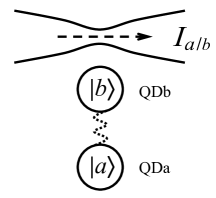
Figure 1: Schematic setup of a solid–state charge qubit measured continuously by a quantum point contact. The qubit is represented by an extra electron tunneling between the coupled quantum dots. The tunneling amplitude of the QPC is susceptible to changes in the surrounding electrostatic environment, and can therefore be used to sense the position of the extra electron.

II Model description

The system under investigation is schematically shown in Fig. 1. The qubit is represented by an extra electron tunneling between two coupled quantum dots (QDa and QDb). When the electron occupies the QDa (QDb), the qubit is said to be in the localized state $|a\rangle$ ($|b\rangle$). A nearby QPC serves as the charge detector to continuously monitor the position of the electron. Occupation of the electron in different dots leads to distinct influence on the transport current through the QPC. It is right this mechanism that makes it possible to read out the qubit-state information. The entire system is described by the Hamiltonian $H_{\rm T}=H_{\rm qu}+H_{\rm D}+H^{\prime}$, where

$$H_{\rm qu}=\frac{1}{2}\epsilon\sigma_{z}+\Omega\sigma_{x},$$ (1a)

$$H_{\rm D}=\sum_{k\in{\rm L}}\varepsilon_{k}\hat{c}_{k}^{\dagger}\hat{c}_{k}+\sum_{q\in{\rm R}}\varepsilon_{q}\hat{c}_{q}^{\dagger}\hat{c}_{q}\,,$$ (1b)

$$H^{\prime}=\sum_{s=a,b}\sum_{k,q}t^{s}_{kq}\hat{c}_{k}^{\dagger}\hat{c}_{q}\cdot|s\rangle\langle s|+{\rm h.c.}.$$ (1c)

Here, $H_{\rm qu}$ denotes the qubit Hamiltonian, where the pseudospin operators are defined as $\sigma_{z}\equiv|a\rangle\langle a|-|b\rangle\langle b|$ and $\sigma_{x}\equiv|a\rangle\langle b|+|b\rangle\langle a|$, respectively. Each dot has only one bound state, i.e., the logic states $|a\rangle$ and $|b\rangle$, with level detuning $\epsilon$ and interdot coupling $\Omega$.

The second component $H_{\rm D}$ depicts the left and right QPC reservoirs, where $\hat{c}_{k}$ ($\hat{c}_{q}$) denotes the annihilation operator for an electron in the left (right) QPC reservoir. The electron reservoirs are characterized by the Fermi distributions $f_{\alpha}{(\omega)}=\{1+e^{\beta(\omega-\mu_{\alpha})}\}^{-1}$, where $\mu_{\alpha}$ is the Fermi energy of the left ($\alpha$=L) or right ($\alpha$=R) reservoir, and $\beta=(k_{\rm B}T)^{-1}$ is the inverse temperature. Hereafter, the Planck’s constant $\hbar$ and the electron charge $e$ are set to unity, i.e. $\hbar=e=1$, unless stated otherwise. Throughout this work, we define $\mu^{\rm eq}_{\rm L}=\mu^{\rm eq}_{\rm R}=0$ for the equilibrium chemical potentials (or Fermi energies) of the QPC reservoirs. An applied measurement voltage thus is modeled by the difference in chemical potentials of the left and right electrodes: $V=\mu_{\rm L}-\mu_{\rm R}$.

The tunneling Hamiltonian for the QPC detector is represented by the last component $H^{\prime}$. The amplitude $t^{s}_{kq}$ of electron tunneling through two reservoirs of the QPC depends explicitly on the qubit state $|s\rangle$ ($s=a$ or $b$). Thus the quantum operator to be measured is $\sigma_{z}$. By denoting $Q_{s}\equiv|s\rangle\langle s|$, the qubit–QPC detector coupling in the $H_{\rm D}$–interaction picture can be rewritten as $H^{\prime}(t)=\sum_{s}[\hat{f}_{s}(t)+\hat{f}^{{\dagger}}_{s}(t)]\cdot Q_{s}$, with $\hat{f}_{s}(t)\equiv e^{{\rm i}H_{\rm D}t}\big{(}\sum_{kq}t_{kq}^{s}\hat{c}_{k}^{\dagger}\hat{c}_{q}\big{)}e^{-{\rm i}H_{\rm D}t}$. The effects of the stochastic QPC reservoirs on measurement are characterized by the reservoir correlation functions $C_{ss^{\prime}}^{(+)}(t-\tau)\equiv\langle\hat{f}_{s}^{\dagger}(t)\hat{f}_{s^{\prime}}(\tau)\rangle$ and $C_{ss^{\prime}}^{(-)}(t-\tau)\equiv\langle\hat{f}_{s}(t)\hat{f}_{s^{\prime}}^{\dagger}(\tau)\rangle$. By introducing the reservoir spectral density function

$$J_{ss^{\prime}}(\omega,\omega^{\prime})=\sum_{k,q}t_{kq}^{s}t_{kq}^{s^{\prime}}\delta(\omega-\varepsilon_{k})\delta(\omega^{\prime}-\varepsilon_{q}),$$ (2)

these QPC coupling correlation functions can be recast as

$$C_{ss^{\prime}}^{(\pm)}(t)=\!\int\!\!\!\int\!\!{\rm d}\omega{\rm d}\omega^{\prime}J_{ss^{\prime}}(\omega,\omega^{\prime})f_{\rm L}^{(\pm)}(\omega)f_{\rm R}^{(\mp)}(\omega^{\prime})e^{\pm{\rm i}(\omega-\omega^{\prime})t},$$ (3)

where $f_{\alpha}^{(+)}(\omega)$ is the usual Fermi function, and $f_{\alpha}^{(-)}(\omega)\equiv 1-f_{\alpha}^{(+)}(\omega)$.

In order to characterize finite cutoff energy of the QPC reservoirs, we introduce a single Lorentzian to model the band structure. For the sake of constructing analytical results, we assume a simple Lorentzian function of cutoff “w” centered at the Fermi energy for the spectral density Eq. (2). Moreover, the bias voltage is conventionally described by a relative shift of the entire energy-bands, thus the centers of the Lorentzian functions would fix at the Fermi levels $\mu_{\rm L}$ and $\mu_{\rm R}$. Without loss of generality, we set Luo et al. (2009)

$$J_{ss^{\prime}}(\omega,\omega^{\prime})=\chi_{s}\chi_{s^{\prime}}\frac{\Gamma_{\rm L}^{0}{\rm w}^{2}}{(\omega-\mu_{\rm L})^{2}+{\rm w}^{2}}\cdot\frac{\Gamma_{\rm R}^{0}{\rm w}^{2}}{(\omega^{\prime}-\mu_{\rm R})^{2}+{\rm w}^{2}},$$ (4)

where $\Gamma_{\rm L}^{0}$ $(\Gamma_{\rm R}^{0})$ is the maximum of the spectral in the left (right) electrode; $\chi_{s}$ and $\chi_{s^{\prime}}$ are qubit-QPC coupling parameters, which are of $\chi_{a}>\chi_{b}$, as can be inferred from Fig. 1. In the limit of w$\rightarrow\infty$, the QPC spectral density Eq. (4) becomes energy-independent and reduces to the constant WBL spectral density used in the literature.

III Non-Markovian Dynamics

The non–Markovian dynamics of the reduced system is described by a generalized time-nonlocal quantum master equation. An equation of this type can be obtained from the partitioning scheme devised by Nakajima and Zwanzig Zwanzig (2001); Breuer and Petruccione (2002), or in the real-time diagrammatic technique for the dynamics of the reduced density matrix on the Keldysh contour Makhlin et al. (2001),

$$\dot{\rho}(t)=-{\rm i}{\cal L}\rho(t)-\!\int_{-\infty}^{t}\!{\rm d}\tau\Pi(t-\tau)\rho(\tau),$$ (5)

where the first term ${\cal L}(\cdots)\equiv[H_{\rm qu},(\cdots)]$ is the qubit Liouvillian. The influence of the QPC detector on the dynamics of the qubit is described by the memory kernel (the second term), which is given by Yan (1998),

$$\!\!\Pi(t-\tau)\rho(\tau)=\sum_{ss^{\prime}}[ Q_{s},C_{ss^{\prime}}(t-\tau)G(t-\tau)Q_{s^{\prime}}\rho(\tau)$$

$$\;\;-C^{\ast}_{ss^{\prime}}(t-\tau)G(t-\tau)\rho(\tau)Q_{s^{\prime}}],$$ (6)

where $C_{ss^{\prime}}(t-\tau)=C^{(+)}_{ss^{\prime}}(t-\tau)+C^{(-)}_{ss^{\prime}}(t-\tau)$, and $G(t-\tau)\equiv e^{-{{\rm i}\cal L}(t-\tau)}$ is the free propagator associated with the qubit Hamiltonian alone. In deriving Eq. (5), the only approximation made is the second-order perturbation in the system-reservoir coupling. This equation thus is valid for arbitrary reservoir temperatures, cutoff energies, and measurement voltages, as long as the second-order perturbation holds.

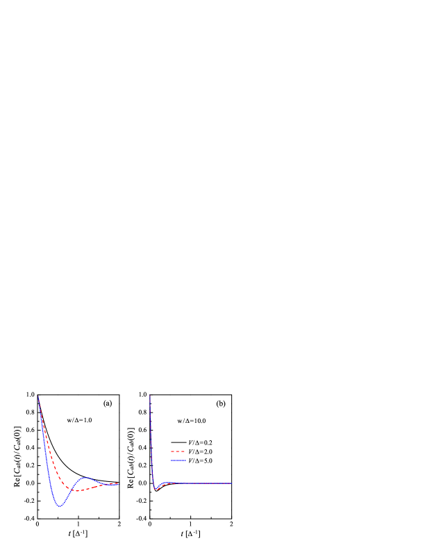
Figure 2: Real part of reservoir correlation function $C_{ab}(t)$ at (a) a small cutoff energy w$/\Delta=1.0$ and (b) a large cutoff energy w$/\Delta=10.0$ for different bias voltages: $V/\Delta=0.2$ (solid lines), $V/\Delta=2.0$ (dashed lines), and $V/\Delta=5.0$ (dotted lines). The temperature is $\beta\Delta=1.0$.

The Markovian approximation is valid only when the correlation time of the reservoir is much shorter than the characteristic time of the reduced quantum system. The former one is defined as the time scale at which the profiles of the QPC reservoir two-time correlation function decays. It is closely associated with the following time scales, the time scale of the QPC spectral density ($\sim$w^-1), the time scale of the applied bias ($\sim V^{-1})$, and the time scale of the QPC reservoir temperature ($\sim\beta$). In what follows, we first study numerically how the reservoir correlation time is varied as a function of different parameters of the QPC reservoirs.

Fig. 2 shows the real parts of the QPC reservoir correlation function $C_{ab}(t)$ versus time for various values of cutoff energy and voltage at a given temperature $\beta\Delta=1.0$. The correlation time decreases as the voltage increases, which is particularly prominent for a narrow cutoff w$/\Delta=1.0$ as displayed in Fig. 2(a). By comparing Fig. 2 (a) and (b), it is revealed that the dependence of reservoir correlation time on the bias voltage is much weaker than that on the cutoff. In the limit of w$\rightarrow 0$, one finds $J_{ss^{\prime}}(\omega,\omega^{\prime})\propto\delta(\omega-\mu_{\rm L})\delta(\omega^{\prime}-\mu_{\rm R})$, which leads to QPC correlation functions proportional to $e^{\pm{\rm i}Vt}$, i.e. completely non-local in time. The opposite limit of WBL (w$\rightarrow\infty$) corresponds to a channel-mixture regime, where a great number of possible transitions of electron tunneling between the two reservoirs of the QPC take place. It was shown in this regime the QPC reservoir correlation time and memory effect are remarkably reduced Lee and Zhang (2008). Thus, the larger the cutoff is, the shorter the correlation time is. The reservoir correlation time is mainly restricted by the cutoff.

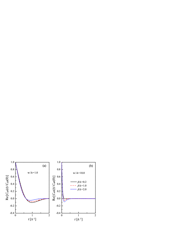
Figure 3: Real part of reservoir correlation function $C_{ab}(t)$ vs time “$t$” for (a) w$/\Delta=10.0$ and (b) w$/\Delta=1.0$ at different temperatures: $\beta\Delta=0.2$ (solid lines), $\beta\Delta=1.0$ (dashed lines), and $\beta\Delta=2.0$ (dotted lines). The measurement voltage is $V/\Delta=2.0$.

To explore the influence of the temperature, we plot in Fig. 3 the reservoir correlation function for various temperatures. Analogous to that on the measurement voltage, the correlation time deceases as the reservoir temperature rises. Nevertheless, the effect of the temperature on the reservoir correlation time is less sensitive than that on the voltage, as can be seen by comparing Fig. 2 and Fig. 3. Therefore, the cutoff energy has the dominant role to play in determining the QPC reservoir correlation time.

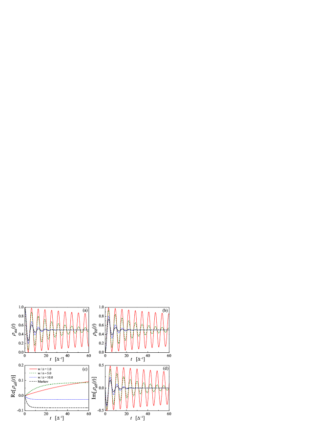
Figure 4: Non-Markovian dynamics of the qubit for different values of cutoff energy: w$/\Delta=1.0$ (solid lines), w$/\Delta=5.0$ (dashed lines), and w$/\Delta=10.0$ (dotted lines). (a) The probability of finding the electron in the localized state $|a\rangle$: $\rho_{aa}(t)\equiv\langle a|\rho(t)|a\rangle$, (b) in the localized state $|b\rangle$: $\rho_{bb}(t)\equiv\langle b|\rho(t)|b\rangle$, (c) real part of the off-diagonal matrix element $\rho_{ab}(t)$, and (d) imaginary part of $\rho_{ab}(t)$. The Markovian WBL results are also plotted in dash-dotted lines for comparison. The qubit is assumed to be symmetric ($\epsilon=0$), and initially in the state $\rho_{\rm ini}=|a\rangle\langle a|$. Other parameters used are $V/\Delta=5.0$, $\beta\Delta=1.0$, $\eta\Delta^{2}=2.0$, and the tunneling amplitudes $\chi_{a}/\Delta=1.0$ and $\chi_{b}/\Delta=0.8$.

With the knowledge of these time scales, we are now in a position to discuss the non-Markovian dynamics of the qubit under the continuous measurement of the QPC. The numerical propagation of the time-nonlocal QME is facilitated by employing the approach of auxiliary density operators Welack et al. (2006); Jin et al. (2008); Croy and Saalmann (2009, 2010). The calculation of the time evolution is then reduced to the propagation of coupled differential equations. The numerical results of the non-Markovian dynamics of the qubit are plotted in Fig. 4 for different values of the cutoff energy. For comparison, we have also plotted the Markovian result by the dash-dotted lines for the same parameters.

The measurement backaction-induced dephasing leads to a coherent to incoherent transition of the qubit electron tunneling. In the coherent regime, the tunneling leads to the well-known Rabi oscillations with frequency given by $\Delta$, as indicated in Fig. 4(a) and (b). For a symmetric qubit ($\epsilon=0$), the occupation probability in each dot finally reaches 1/2 for both Markovian and non-Markovian cases. However, for a small cutoff, such as w$/\Delta=1.0$ (solid lines), the non-Markovian relaxation behavior shows a considerable difference to the Markovian case (dash-dotted lines). As the cutoff energy increases, the qubit relaxation gets close to that of the Markovian result, due to reduced reservoir correlation time [see the dotted lines in Fig. 4(a) and (b)].

The backaction-induced dephasing behavior is described by the off-diagonal density-matrix element, as displayed in Fig. 4(c) and (d). The real part of $\rho_{ab}$ approaches a nonzero constant at long times. The nonzero stationary result stems from the energy exchange between the qubit and QPC detector Li et al. (2004, 2005); Luo et al. (2009). For both Markovian and non-Markovian cases, the imaginary part of $\rho_{ab}$ goes to zero in the stationary limit. However, for a small cutoff energy, the dephasing rate is much lower than that of the Markovian case, as displayed by the solid line in Fig. 4(d). In Markovian processes, information flows continuously from the qubit to its environment. Yet, in the presence of non-Markovian behavior, a reversed flow of information from the environment back to the reduced system occurs, which leads to the reduction of the dephasing rate.

To clearly demonstrate this unique feature, we employ the “trace distance” of two quantum states $\rho_{1}$ and $\rho_{2}$, which is defined as Nielsen and Chuang (2000); Breuer et al. (2009); Laine et al. (2010)

$$D[\rho_{1}(t),\rho_{2}(t)]=\frac{1}{2}{\rm tr}|\rho_{1}(t)-\rho_{2}(t)|.$$ (7)

Here the norm is given by $|A|=\sqrt{A^{\dagger}A}$, and $\rho_{1,2}(t)$ are the dynamical qubit states for a given pair of initial states $\rho_{1,2}(0)$. The trace distance describes the probability of distinguishing those states. In Markovian processes, the distinguishability between any two states are continuously reduced, and thus the trace distance $D(\rho_{1},\rho_{2})$ decreases monotonically. The essential property of non-Markovian behavior is the growth of this distinguishability. An increase of the trace distance during any time intervals implies the emergence of non-Markovianity (inverse flow of the information). One is therefore inspired to utilize the rate of change of the trace distance “$\kappa$” to exhibit unambiguously this process

$$\kappa[t,\rho_{1,2}(0)]=\frac{{\rm d}}{{\rm d}t}D[\rho_{1}(t),\rho_{2}(t)].$$ (8)

Apparently, for a Markovian process the monotonically reduction of the trace-distance implies $\kappa\leq 0$. The existence of $\kappa>0$ during any time intervals identifies the non-Markovian process.

The numerical results are plotted in Fig. 5. For a small cutoff energy (w$/\Delta=1.0$) as shown in Fig. 5(a), there exist certain times in which $\kappa>0$. In those regimes, the information flows from the environment back to the reduced system, i.e. the non-Markovian process. It explains the suppression of the dephasing rate in Fig. 4(d). An increase in cutoff energy reduces reservoir correlation time, and thus leads to the inhibition of the non-Markovianity [see Fig. 5(b) for w$/\Delta=10.0$]. While in Markovian processes, measurements tend to wash out more and more characteristic features of the two states, resulting thus in an uncovering of these features. The rate of change of the trace distance “$\kappa$” stays below zero, as shown in Fig. 5(c). The suppression of the dephasing rate due to non-Markovian dynamics has an important impact on noise characteristics of the measurement, which will be discussed in the next section.

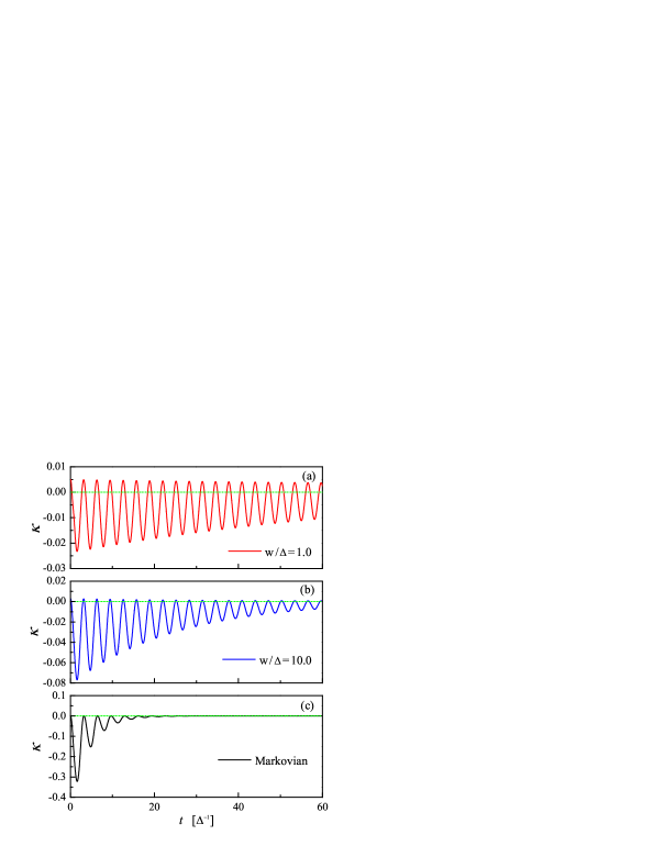
Figure 5: The rate of change $\kappa$ of the trace distance as a function of time for (a) w$/\Delta=1.0$, (b) w$/\Delta=10.0$, and (c) Markovian WBL result. The initial pair of states used are $\rho_{1}(0)=|a\rangle\langle a|$ and $\rho_{2}(0)=|b\rangle\langle b|$. The other parameters are the same as those in Fig. 4.

IV Noise Characteristics

In this section, we first introduce the “$N$”-resolved non-Markovian master equation for the calculation of the output noise characteristics of the QPC detector. Next, the numerical results for QPC noise are presented, with special emphasis on the measurement SNR under various conditions.

IV.1 Particle-Number-Resolved Master Equation

To achieve the description of the output characteristics, the reduced density matrix $\rho(t)$ is unraveled into components $\rho^{(N)}(t)$, in which “$N$” is the number of electrons passing though the QPC during the time span $[0,t]$. The resultant time-nonlocal “$N$”–resolved quantum master equation reads Makhlin et al. (2001); Flindt et al. (2008); Aguado and Brandes (2004); Braggio et al. (2006); Jin et al. (2011)

$$\dot{\rho}^{(N)}(t)=-{\rm i}{\cal L}\rho^{(N)}(t)-\!\int_{0}^{t}\!{\rm d}\tau\bigg{\{}\Pi_{0}(t-\tau)\rho^{(N)}(\tau)-\sum_{\pm}\Pi_{\pm}(t-\tau)\rho^{(N\pm 1)}(\tau)\bigg{\}}+\varrho^{(N)}(t),$$ (9)

with

$$\Pi_{0}(t-\tau)(\cdots)=\sum_{ss^{\prime}}\{C_{ss^{\prime}}(t-\tau)Q_{s}G(t-\tau)Q_{s^{\prime}}(\cdots)+[C_{ss^{\prime}}(t-\tau)]^{\ast}G(t-\tau)(\cdots)Q_{s^{\prime}}Q_{s}\},$$ (10a)

$$\Pi_{\pm}(t\!-\!\tau)(\cdots)=\sum_{ss^{\prime}}\{C^{(\pm)}_{ss^{\prime}}(t-\tau)G(t-\tau)Q_{s^{\prime}}(\cdots)Q_{s}+[C^{(\pm)}_{ss^{\prime}}(t-\tau)]^{\ast}Q_{s}G(t\!-\!\tau)(\cdots)Q_{s^{\prime}}\}.$$ (10b)

Here, the memory kernel $\Pi_{0}$ corresponds to “continuous” evolution of the system, and $\Pi_{\pm}$ denotes forward and backward jumps of the transfer of an electron from the left electrode to the right one. By summing up Eq. (9) over all possible electron numbers “$N$”, one straightforwardly recovers the unconditional master equation (5). Hereafter, we assume that the system evolves from $t_{0}=-\infty$, such that the electronic occupation probabilities at $t=0$, where electron counting begins, have reached the stationary state, i.e., $\rho^{(N)}(t=0)=\delta_{N,0}\rho_{\rm st}$, with $\rho_{\rm st}=\rho(t\rightarrow\infty)$. The effects of the memory of its history prior to time $t=0$ are incorporated in the inhomogeneity $\varrho^{(N)}$ Emary and Aguado (2011).

The unraveling of the density matrix in Eq. (9) enables us to evaluate the probability distribution for the number of transferred charge $P(N,t)={\rm tr}\{\rho^{(N)}(t)\}$, where the trace is over degrees of freedom of the reduced system. In principle, all the cumulants of the current distribution can be obtained, consisting thus a spectrum of full counting statistics. For instance, the first cumulant is directly related to the average current through the QPC, $I(t)=\sum_{N}N\dot{P}(N,t)$. By using Eq. (9), the current is given by

$$I(t)=\int_{0}^{t}{\rm d}\tau\,{\rm tr}\{[\Pi_{-}(t-\tau)-\Pi_{+}(t-\tau)]\rho(\tau)\}.$$ (11)

The stationary current thus reads

$$\bar{I}\equiv I(t\rightarrow\infty)={\rm tr}\{J_{-}(z)\rho_{\rm st}\}|_{z\rightarrow 0},$$ (12)

with

$$J_{\pm}(z)=\tilde{\Pi}_{-}(z)\pm\tilde{\Pi}_{+}(z).$$ (13)

Here $\tilde{\Pi}_{0}(z)$ and $\tilde{\Pi}_{\pm}(z)$, the resolvents of the corresponding kernels in Eq. (9), are obtained by performing the Laplace transform

$$\!{\tilde{\Pi}}_{0}(z)(\cdots)=\sum_{ss^{\prime}}\Big{\{} Q_{s}\,\tilde{{\cal Q}}_{ss^{\prime}}(z+{\rm i}{\cal L})Q_{s^{\prime}}(\cdots)$$

$$+\tilde{{\cal Q}}_{ss^{\prime}}(z^{\ast}-{\rm i}{\cal L})(\cdots)\,Q_{s^{\prime}}Q_{s}\Big{\}},$$ (14a)

$$\!{\tilde{\Pi}}_{\pm}(z)(\cdots)=\sum_{ss^{\prime}}\Big{\{} \tilde{{\cal Q}}^{(\pm)}_{ss^{\prime}}(z+{\rm i}{\cal L})Q_{s^{\prime}}(\cdots)Q_{s}$$

$$+\!Q_{s}\tilde{{\cal Q}}^{(\pm)}_{ss^{\prime}}(z^{\ast}-{\rm i}{\cal L})(\cdots)Q_{s^{\prime}}\Big{\}},$$ (14b)

where ${\cal Q}_{ss^{\prime}}={\cal Q}_{ss^{\prime}}^{(+)}+{\cal Q}_{ss^{\prime}}^{(-)}$, with

$$\tilde{\mathcal{Q}}_{ss^{\prime}}^{(\pm)}(z)\equiv\int_{0}^{\infty}{\rm d}tC_{ss^{\prime}}^{(\pm)}(t)e^{-zt}.$$ (15)

In the limit $z\rightarrow{\rm i}\omega$, it can be further simplified to

$$\tilde{\mathcal{Q}}_{ss^{\prime}}^{(\pm)}(z)|_{z\rightarrow{\rm i}\omega}=\tilde{C}^{(\pm)}_{ss^{\prime}}(\omega)+{\rm i}\tilde{D}^{(\pm)}_{ss^{\prime}}(\omega).$$ (16)

The first term denotes the coupling spectral function

$$\tilde{C}^{(\pm)}_{ss^{\prime}}(\omega)\equiv\int_{-\infty}^{\infty}{\rm d}tC_{ss^{\prime}}^{(\pm)}(t)e^{-{\rm i}\omega t},$$ (17)

which is associated with particle transfer processes, with interactions between the qubit and QPC being properly accounted for. For a Lorentzian band structure [see Eq. (4)], it can be evaluated explicitly as

$$\tilde{C}_{ss^{\prime}}^{(\pm)}(\omega)= \frac{\eta\chi_{s}\chi_{s^{\prime}}}{e^{\beta(\omega\pm V)}-1}\frac{4{\rm w}^{2}}{(\omega\pm V)^{2}+4{\rm w}^{2}}\bigg{\{}\frac{{\rm w}}{2}\varphi(\omega\pm V)$$

$$+\frac{{\rm w}^{2}}{\omega\pm V}[\phi(\omega\pm V)-\phi(0)]\bigg{\}},$$ (18)

where $\eta=2\pi\Gamma_{\rm L}^{0}\Gamma_{\rm R}^{0}$, $\phi(x)$ and $\varphi(x)$ denote the real and imaginary parts of the digamma function $\Psi(\frac{1}{2}+\beta\frac{{\rm w}+{\rm i}x}{2\pi})$, respectively. Note here due to finite cutoff energy of the QPC detector and quasistep feature in the Fermi functions in Eq. (3), $\tilde{\mathcal{Q}}_{ss^{\prime}}^{(\pm)}(\omega)$ decays exponentially when $\omega$ goes beyond the cutoff energy. As a result, the resolvents of the kernels $\tilde{\Pi}_{0}(z)$ and $\tilde{\Pi}_{\pm}(z)$ vanish in the limit $\omega\rightarrow\infty$. It should also be stressed that the present spectrum functions satisfy the detailed–balance relation, i.e. $\tilde{C}_{ss^{\prime}}^{(+)}(\omega)=e^{-\beta(\omega+V)}\tilde{C}_{ss^{\prime}}^{(-)}(-\omega)$, which means that our approach properly accounts for the energy exchange between the qubit and the detector during measurement. This is the reason we get nonzero stationary value for the real part of the off-diagonal matrix element $\rho_{ab}$, in contrast to that obtained in Ref. Gurvitz, 1997.

With the Knowledge of the spectral function, the dispersion function $\tilde{D}_{ss^{\prime}}^{(\pm)}(\omega)$ can be obtained via the Kramers-Kronig relation

$$\tilde{D}_{ss^{\prime}}^{(\pm)}(\omega)=\frac{1}{\pi}\,{\cal P}\!\!\int_{-\infty}^{\infty}d\omega^{\prime}\frac{\tilde{C}_{ss^{\prime}}^{(\pm)}(\omega^{\prime})}{\omega-\omega^{\prime}},$$ (19)

where ${\cal P}$ stands for Cauchy’s principal value. Physically, the dispersion accounts for the coupling-induced energy renormalization of the internal energies Xu and Yan (2002); Yan and Xu (2005); Caldeira and Leggett (1983); Weiss (2008).

The second cumulant of the current distribution corresponds to the shot noise. To study the finite-frequency spectrum, we employ the MacDonald’s formula MacDonald (1962)

$$S(\omega)=2\omega\int_{0}^{\infty}{\rm d}t\sin(\omega t)\frac{{\rm d}}{{\rm d}t}[\langle N^{2}(t)\rangle-(\bar{I}t)^{2}],$$ (20)

with $\langle N^{2}(t)\rangle\equiv\sum_{N}N^{2}P(N,t)$. By utilizing Eq. (9), it is simplified to

$$S(\omega)=S_{0}+4\omega{\rm Im}[{\rm tr}\{J_{-}(z)\tilde{N}(z)\}]|_{z\rightarrow{\rm i}\omega},$$ (21)

where the noise pedestal $S_{0}=2{\rm tr}\{J_{+}(0){\rho}_{\rm st}\}$ is the shot noise of the QPC detector alone. In the WBL and large voltage, it reproduces the well-known result $S_{0}=2e\bar{I}$ Korotkov (1999). Rich information about qubit measurement dynamics is contained in the excess noise (second term) in Eq. (21). Here, $\tilde{N}(z)$ is the Laplace space counterpart of $N(t)\equiv\sum_{N}N\rho^{(N)}(t)$. By employing the “$N$”-resolved quantum master equation (9), it can be solved from the following algebraic equation

$$z\tilde{N}(z)=-{\rm i}{\cal L}\tilde{N}(z)-\tilde{\Pi}(z)\tilde{N}(z)+\frac{J_{-}(0)\tilde{\rho}_{\rm st}}{z},$$ (22)

with $\tilde{\Pi}(z)\equiv\tilde{\Pi}_{0}(z)-\tilde{\Pi}_{+}(z)-\tilde{\Pi}_{-}(z)$.

IV.2 Noise characteristics

The basic physics of the measurement process is the trade–off between acquisition of information about the state of the qubit and backaction dephasing of this system. For a quantum-limited detector, the rates of the two processes coincide, while for a less efficient detector, the qubit dephasing is more rapid than information acquisition. It imposes a fundamental limit on the SNR for a weakly measured qubit, known as the K-A bound Korotkov and Averin (2001). An interesting feature is that the K-A bound is closely related to oscillation peak (around the hybridization energy $\Delta=\sqrt{\epsilon^{2}+(2\Omega)^{2}}$) in the noise spectrum of the QPC detector, i.e. the maximum peak height can reach 4 times larger than the noise pedestal for a quantum-limited detector.

To see how this bound emerges, let us first briefly derive this inequality for the Markovian case. We start with the current-correlation function $K(t)=\langle\hat{I}(t+\tau)\hat{I}(t)\rangle_{t\rightarrow\infty}$, where the average is taken over the whole system. The evolution of the QPC current operator $\hat{I}(t)$ is determined by the entire system Hamiltonian, which yields Korotkov and Averin (2001)

$$K(\tau)=e\bar{I}\delta(\tau)+\frac{(\delta I)^{2}}{4}{\rm tr}[\sigma_{z}\sigma_{z}(\tau)\rho_{\rm st}],$$ (23)

with $\bar{I}$ the stationary current and $\rho_{\rm st}$ is the steady state of the qubit. The tr[$\cdots$] denotes the trace over the state of the reduced system. The current change $\delta I=I_{a}-I_{b}$ reflects the current response to electron oscillations between the dots, where $I_{a}(I_{b})$ corresponds to the QPC current when the electron occupies the state $|a\rangle(|b\rangle)$. Apparently, $K(\tau)$ reflects the correlation function of the electron position in the dots given by $\sigma_{z}$. The evolution of the $\sigma_{z}(\tau)$ can be found by expanding the evolution operator of the entire system to the second order in the coupling constant, and then averaging over the reservoir states to obtain the equations of motion, with dephasing rate given by $\Gamma_{\rm d}$. In the case of $\epsilon=0$, the noise spectrum is given by Korotkov and Averin (2001)

$$S(\omega)=S_{0}+\frac{(\delta I)^{2}\Gamma_{\rm d}\Delta^{2}}{(\omega^{2}-\Delta^{2})^{2}+\Gamma_{\rm d}^{2}\omega^{2}},$$ (24)

where $S_{0}=2e\bar{I}$ is the output noise of the QPC detector alone, i.e. the noise pedestal. At the qubit oscillation frequency $\omega=\Delta$, the noise spectrum has a maximum “signal” of $(\delta I)^{2}/\Gamma_{\rm d}$. The SNR thus is limited:

$${\rm SNR}\equiv\frac{S(\Delta)-S_{0}}{S_{0}}\leq 4.$$ (25)

This is the K-A bound. It has been confirmed in Refs. Goan and Milburn, 2001; Ruskov and Korotkov, 2003; Shnirman et al., 2004, generalized in Refs. Mao et al., 2004, 2005, and measured in Ref. Il’ichev et al., 2003. However, several schemes have been proposed recently to overcome the K-A bound, which can be divided into two categories. The first one concerns with increasing the signal, such as quantum nondemolition measurements Averin (2002); Jordan and Büttiker (2005a) and quantum feedback control Wang et al. (2007b); Vijay et al. (2012). The second type is to reduce the pedestal noise by employing a strongly responding SET Jiao et al. (2009) or twin detectors Jordan and Büttiker (2005b). In this work, we find the non-Markovian processes allow a violation of the K-A bound on the SNR. The details together with an interpretation will be provided later.

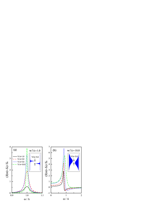
Figure 6: Noise feature for a symmetric qubit ($\epsilon=0$) under different measurement voltages for (a) w$/\Delta=1.0$ and (b) w$/\Delta=10.0$. The inset in (a) and (b) shows the reservoir’s spectral density for corresponding cutoff energies and fixed measurement voltage $V/\Delta=5.0$. The temperature and other parameters are the same as those in Fig. 4.

The computed noise is shown in Fig. 6 for different cutoff energies and voltages. For a small cutoff energy (w$/\Delta=1.0$), prominent non-Markovian processes take place, which leads to a strongly suppressed dephasing rate [cf. Fig. 4(d)]. It is reflected in the noise spectrum as the narrow width of the oscillation peak. As the measurement voltage increases, the qubit will be excited, which leads to the rising peak height (“signal”) and SNR. However, the SNR cannot exceed the limit of “4”, even in the limit of $V/\Delta\rightarrow\infty$, as we have verified.

In the case of large cutoff energy (w$/\Delta=10.0$), however, violation the K-A bound is observed unambiguously [see, for instance, the dotted curve in Fig. 6(b)]. The violation is due to the presence of non-Markovian processes, in which reversed flow of information from the environment back to the reduced system takes place. This mechanism is analogous to the quantum feedback scheme Wang et al. (2007b); Vijay et al. (2012). Yet, there, one has to implement an extra procedure in which the measurement information in the detector is converted into the evolution of a qubit state. Our analysis thus serves a direct and transparent way to improve the efficiency in quantum measurement.

One may ask why the K-A bound is not violated in the case of a small cutoff (w$/\Delta=1.0$), where prominent non-Markovian processes are present. This is actually associated with the energy that needed to excite the qubit. Let us consider the situation of a voltage $V/\Delta=5.0$. For a small cutoff (w$/\Delta=1.0$), the number of channels for electrons to tunnel though the detector is remarkably suppressed, see the schematic density spectral in the inset of Fig. 6(a). It restricts the number of electrons that can provide energy to excite the qubit, and eventually results in the SNR below the limit of “4”. Unlike the cases of w$/\Delta=1.0$, the number of channels are considerably increased for a large cutoff energy (w$/\Delta=10.0$), as shown in the inset of Fig. 6(b). Therefore, sufficient energy is provided to excite the qubit, which leads eventually to the violation of the K-A bound. However, even in the case of large cutoff energy, the number of channels does not necessarily increase with rising voltage. For instance, there are less effective channels in the case of $V/\Delta=10.0$ than that of $V/\Delta=5.0$. One thus observes a suppressed SNR for $V/\Delta=10.0$ in comparison with that of $V/\Delta=5.0$, as shown by the dot-dashed curve in Fig. 6(b).

Furthermore, the qubit-QPC coupling gives rise to a dynamical renormalization of the qubit energies [see Eq. (19)], which vanishes at “w$\rightarrow 0$ and increases with the cutoff Luo et al. (2009). On one hand, it leads to the shift of the oscillation peaks towards low frequencies, as shown in Fig. 6(b). One the other hand, the energy renormalization gives rise to incoherent jumps between the two states. The detector attempts to localize the electron in one of the states for a longer time, leading thus to the quantum Zeno effect, which is manifested as the non-zero noise at zero frequency, as displayed in Fig. 6(b).

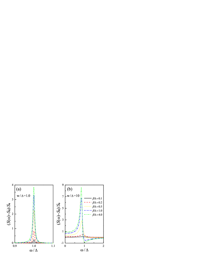
Figure 7: Noise spectrum of a symmetric qubit at various temperatures and cutoff energies (a) w$/\Delta=1.0$ and (b) w$/\Delta=10.0$. The measurement voltage is $V/\Delta=5.0$. The other parameters are the same as those in Fig. 4.

We are now in a position to discuss the influence of the temperature on the noise spectrum. The numerical results are plotted in Fig. 7. For a small cutoff energy (w$/\Delta=1.0$), the presence of a prominent non-Markovian effect inhibits the dephasing rate, which is insensitive to the temperature, as shown in Fig. 3(b). The width of the oscillation peak thus is strongly suppressed for all the temperatures. Furthermore, it is found that the height of the oscillation peak decreases rapidly with rising temperature. The reason is attributed to the enhanced qubit relaxation rate as the temperature grows, analogous to the finding in the the Markovian limit Li et al. (2005). In this regime of small cutoff energy, the SNR cannot exceed the K-A bound as we have checked. It is again owing to the limited number of channels that electrons can transfer through the QPC. However, in the case of large bandwidth w$/\Delta=10.0$ strong violation of the K-A bond is observed at a low temperature $\beta\Delta=4.0$ [see Fig. 7(b)]. As the temperature grows, the oscillation peak is again reduced due to qubit relaxation, similar to the situation of w$/\Delta=1.0$.

To complete this section, we discuss the situation under which the violation of the K-A bound may take place. In the case of small cutoff energy (w$<\Delta$), the SNR cannot exceed the limit of “4” under arbitrary voltage and temperature, even though there is a strong non-Markovian effect. It is ascribed to the limited number of channels that electrons can transfer though the detector. It cannot provide enough energy to fully excite the qubit, thus restricts the “efficiency” of the measurement. In this sense, a small cutoff energy works as a suppression mechanism to the “effectiveness” of the voltage and temperature. In the opposite WBL (w$\rightarrow\infty$), one expects very short reservoir correlation time, approaching thus to the Markovian case. Our result reproduces to the previous Markovian ones. In this case, the information flows purely from the reduced system to the reservoir and the SNR is limited to 4. Therefore, the violation of the K-A bound only occurs for moderate cutoff energies, together with an appropriately large measurement voltage and a low temperature. In this regime, enough energy will be provided to excite the qubit, while relaxation to the ground state takes places slowly. Moreover, the presence of finite non-Markovian dynamics results in the opportunity for the information to flow from the reservoir back to the system, which eventually lead to an SNR exceeding the K-A bound. In comparison with the quantum feedback scheme, the present work serves as a straightforward and transparent way to improve the “efficiency” in quantum measurement.

V Conclusions

In summary, we have investigated the dynamics of a charge qubit under continuous measurement by a quantum point contact, with special attention paid to the non-Markovian measurement characteristics. We identified the regimes where prominent non-Markovian memory effects are present by analyzing how the reservoir’s correlation time is varied as function of different parameters of the QPC detector. In comparison with the Markovian case, considerable differences in qubit relaxation and dephasing behaviors were observed in the non-Markovian domain. Furthermore, the non-Markovian dynamics was found to have a vital role to play in the output noise features of the detector. In particular, we observed unambiguously that the signal-to-noise ratio can exceed the limit of “4”, leading thus to the violation of the Korotkov-Averin bound. In comparison with other approaches, such as quantum feedback scheme, our results might open new possibilities to enhance measurement efficiency in a straightforward and transparent way.