Meta-models for structural reliability and uncertainty quantification

Abstract

A meta-model (or a surrogate model) is the modern name for what was traditionally called a response surface. It is intended to mimic the behaviour of a computational model ${\mathcal{M}}$ (e.g. a finite element model in mechanics) while being inexpensive to evaluate, in contrast to the original model ${\mathcal{M}}$ which may take hours or even days of computer processing time. In this paper various types of meta-models that have been used in the last decade in the context of structural reliability are reviewed. More specifically classical polynomial response surfaces, polynomial chaos expansions and kriging are addressed. It is shown how the need for error estimates and adaptivity in their construction has brought this type of approaches to a high level of efficiency. A new technique that solves the problem of the potential biasedness in the estimation of a probability of failure through the use of meta-models is finally presented.

Fifth Asian-Pacific Symposium on Structural Reliability and its Applications (5APSSRA).
Edited by Phoon, K. K., Beer, M., Quek, S. T. & Pang, S. D.2011981-973-0000-00-0

1 Introduction

The coupling of mechanical models and probabilistic approaches has gain a lot of interest in the literature in the last 30 years. More specifically the field of structural reliability has emerged in the mid 70’s in order to provide methods for assessing structures by accounting for uncertainties in both the models and the parameters describing the structures (e.g. geometrical parameters, material properties and applied forces). Structural reliability is nowadays a mature field with industrial applications in domains ranging from civil, environmental, mechanical & aero-space engineering (Ditlevsen and Madsen, 1996). It has given a sound basis for the semi-probabilistic structural codes such as the Eurocodes and has lead to performance-based engineering.

In the last 10 years the field of stochastic spectral methods has blown up based on the pioneering work by Ghanem and Spanos (1991). It has become a field in itself which is at the interface of computational physics, statistics and applied mathematics as shown in the literature on this topic, which is published in scientific journals of these various domains, namely Prob. Eng. Mech., Structural Safety, Reliab. Eng. Sys. Safety, J. Comput. Phys., Comput. Methods Appl. Mech. Engrg., Comm. Comput. Physics on the one hand, SIAM J. Sci. Comput., SIAM J. Num. Anal., J. Royal Stat. Soc. on the other hand, among others.

The large majority of computational methods associated with structural safety and uncertainty quantification rely upon repeated calls to the underlying computational model of the structure or system. For instance Monte Carlo simulation is based on the sampling of the input parameters according to their distribution, and the evaluation of the model response (or system performance in the context of reliability) for each realization. The large number of calls that is required for precise predictions is usually not compatible with costly computational models such as finite element models, even when high-performance computing platforms are at hand. This has opened a new field of research broadly called meta-modelling. This is the goal of this paper to provide some overview of meta-modelling techniques with a focus on their use in structural reliability.

The paper is organized as follows. Section 2 describes the ingredients of uncertainty quantification and recalls the limitations of Monte Carlo simulation for structural reliability analysis. Section 3 describes the general philosophy of meta-modelling and addresses in details three types of meta-models: polynomial response surfaces, polynomial chaos expansions and kriging. Section 4 shows how a meta-model can be used in the context of importance sampling in order to provide unbiased estimators of a probability of failure. Finally Section 5 gathers some application examples.

2 Problem statement

2.1 Computational model

Let us consider a mechanical system whose behavior is modelled by a set of governing equations, e.g. partial differential equations describing its evolution in time. After proper discretization using e.g. a finite element (resp. finite difference) scheme, and using some suitable solving scheme, the computational model may be cast as follows:

$$\boldsymbol{y}={\mathcal{M}}(\boldsymbol{x})$$ (1)

In this equation $\boldsymbol{x}\in{\mathcal{D}}_{\boldsymbol{X}}\in\textrm{I\!R}^{M}$ is a vector describing the input parameters of the model. It usually gathers the parameters describing the geometry of the system, the constitutive laws of the materials and the applied loading. Vector $\boldsymbol{y}\in\textrm{I\!R}^{Q}$ gathers the response quantities which may contain:

• the displacement vector or selected components of the latter;

• the components of the strain (resp. stress) tensor at specific points;

• internal variables (e.g. plastic strain, damage variables, etc.);

• a combination of the latter, at a specific point-in-time or at various time instants.

In the sequel the computational model ${\mathcal{M}}$ is considered as a black box, which is only known point-by-point: if a given set of input parameters $\boldsymbol{x}_{0}$ is selected, running the model provides a unique response vector. It is also assumed that this model is purely deterministic: running twice the model using the same input vector will yield exactly the same output.

Note that in practice evaluating such a computational model may be almost instantaneous if some analytical solution to the constitutive equations exists, whereas it can take hours on high performance computers if it results from a large size finite element model (or a workflow of chained models).

In the sequel the various methods reviewed for uncertainty quantification and reliability analysis consider that the model cannot be modified by the analyst but only run for a set of input vectors. These methods are termed non intrusive in the context of uncertainty propagation.

2.2 Probabilistic model

Let us consider that the uncertainties in the model input parameters are modelled by a random vector $\boldsymbol{X}$ with support ${\mathcal{D}}_{\boldsymbol{X}}\in\textrm{I\!R}^{M}$ and prescribed probability density function $f_{\boldsymbol{X}}(\boldsymbol{x})$. It is beyond the scope of this paper to describe in details how such a probabilistic model can be built from the available information (resp. data). However the following guidelines may be found in the literature:

• When some natural variability of a parameter is evidenced through a set of measured values, the classical approach consists in using statistical inference methods in order to fit the best distribution selected among one or several families (e.g. Gaussian, lognormal, Gamma, Weibull, etc.) using e.g. the maximum likelihood principle. The goodness-of-fit shall be checked using appropriate tests (Stuart et al., 1999). Eventually the best distribution may be selected using criteria such as the Akaike (resp. Bayesian) information criterion (Akaike, 1973; Schwartz, 1978).

• In contrast when no data is available, expert judgment should be resorted to. The available information may be “objectively” modelled using the principle of maximum entropy (Jaynes, 1982; Kapur and Kesavan, 1992). Guidelines such as the JCSS probabilistic model code (Vrouwenvelder, 1997) are available in the literature for modelling loads and material properties in civil engineering (see updated versions of the code at http://www.jcss.byg.dtu.dk).

• In situations where few data is available, a prior expert judgment can be combined with measurements using the framework of Bayesian statistics.

2.3 Structural reliability

In structural reliability analysis the performance of the system is mathematically described by a failure criterion which depends on:

• the (uncertain) mechanical response of the system, say ${\mathcal{M}}(\boldsymbol{X})$;

• possibly additional deterministic parameters $\boldsymbol{d}$ (e.g. a codified threshold) or random variables $\boldsymbol{X}^{\prime}$ (e.g. uncertain resistance)

The failure criterion is mathematically represented by a limit state function (also called performance function) which is conventionally defined as follows:

• The set of parameters $\{\boldsymbol{x},{\boldsymbol{x}^{\prime}},\boldsymbol{d}\}$ such that $g\left({\mathcal{M}}({\boldsymbol{x}}),\boldsymbol{x}^{\prime},\boldsymbol{d}\right)>0$ defines the safe domain ${\mathcal{D}}_{s}$.

• The set of parameters $\{\boldsymbol{x},{\boldsymbol{x}^{\prime}},\boldsymbol{d}\}$ such that $g\left({\mathcal{M}}({\boldsymbol{x}}),\boldsymbol{x}^{\prime},\boldsymbol{d}\right)\leq 0$ defines the failure domain ${\mathcal{D}}_{f}$.

• The limit state surface corresponds to the zero-level of the $g$-function.

Gathering all the parameters into a single notation $\boldsymbol{x}\in{\mathcal{D}}_{\boldsymbol{X}}\subset\textrm{I\!R}^{M}$ for the sake of simplicity, the probability of failure of the system is defined by:

$$P_{f}=\textrm{I\!P}\left[g(\boldsymbol{X})\leq 0\right]=\int_{{\mathcal{D}}_{f}=\left\{\boldsymbol{x}:g(\boldsymbol{x})\leq 0\right\}}f_{\boldsymbol{X}}(\boldsymbol{x})\,d\boldsymbol{x}$$ (2)

The main difficulty in evaluating the probability of failure in Eq.(2) leads in the fact that the integration domain is defined implicitely. Moreover the dimension of the integral is equal to the number of uncertain parameters $M$ which is usually large.

2.4 Classical computational methods

2.4.1 Monte Carlo simulation

Monte Carlo simulation is the basic and universal approach to solving the reliability problem (Rubinstein and Kroese, 2008). Recasting Eq.(2) as:

$$P_{f}=\int_{\textrm{I\!R}^{M}}\boldsymbol{1}_{{\mathcal{D}}_{f}}(\boldsymbol{x})\,f_{\boldsymbol{X}}(\boldsymbol{x})\,d\boldsymbol{x}\equiv\textrm{I\!E}\left[\boldsymbol{1}_{{\mathcal{D}}_{f}}(\boldsymbol{X})\right]$$ (3)

the probability of failure is equal to the expectation of the indicator function of the failure domain, which may be given the following estimator using a $N$-sample $\mathfrak{X}=\left\{\boldsymbol{X}^{(k)},\;k=1,\,\dots\,,N\right\}$ made of $N$ independent copies of $X$:

$${\hat{P}_{f}}=\frac{1}{N}\sum\limits_{k=1}^{N}1_{{\mathcal{D}}_{f}}\,\left(\boldsymbol{X}^{(k)}\right)=\frac{N_{f}}{N}$$ (4)

where $N_{f}$ is the number of samples that fall into the failure domain. This estimator is unbiased and mean-square convergent, since its variance $\displaystyle{{\rm Var}\left[\hat{P}_{f}\right]=P_{f}(1-P_{f})/N}$. The slow convergence rate $\propto 1/\sqrt{N}$ makes the approach particularly inefficient. It is easily shown that the coefficient of variation of the estimator reads:

$$CV_{P_{f}}\equiv\frac{\sqrt{{\rm Var}\left[\hat{P}_{f}\right]}}{\textrm{I\!E}\left[\hat{P}_{f}\right]}\approx\frac{1}{\sqrt{N\,P_{f}}}$$ (5)

From the above equation one can see that a typical evaluation of a probability of failure of the order of magnitude $10^{-r}$ with $CV_{P_{f}}\leq 10\%$ requires about $10^{r+2}$ simulations. This number is not affordable for low probabilities ($10^{-3}-10^{-6}$) as soon as the computational cost of each evaluation of $g$ (which includes a run of ${\mathcal{M}}$) is non negligible, e.g. when finite element analysis is involved.

2.4.2 Beyond Monte Carlo simulation

Various methods have been proposed in the past 30 years in order to solve the reliability problem efficiently. Broadly speaking they can be classified as follows:

• methods that aim at decreasing the computational cost after introducing some approximation in the reliability estimation. The First Order (resp. Second Order) reliability methods (FORM/SORM) are well established in this area, see Hasofer and Lind (1974); Rackwitz and Fiessler (1978); Breitung (1984); Hohenbichler et al. (1987); Breitung (1989); Der Kiureghian et al. (1987); Der Kiureghian and de Stefano (1991) among others.

• methods that are derived from Monte Carlo simulation with the goal of improving the convergence: directional simulation (Ditlevsen et al., 1987; Bjerager, 1988), importance sampling (Hohenbichler and Rackwitz, 1988; Melchers, 1990; Maes et al., 1993; Au and Beck, 1999) and more recently subset simulation (Au and Beck, 2001; Katafygiotis and Cheung, 2005; Hsu and Ching, 2010) and line sampling (Pradlwarter et al., 2007).

• Methods that rely on the use of a surrogate model $\tilde{{\mathcal{M}}}$ which is fast to evaluate and may be used in place of the original model ${\mathcal{M}}$ for reliability analysis

A detailed presentation of the various classical methods can be found in the textbooks by Ditlevsen and Madsen (1996); Melchers (1999); Lemaire (2009). This is the aim of the present paper to address the last point and review different classes of surrogate models and their use in structural reliability.

3 Meta-models for structural reliability

3.1 Introduction

As introduced above, a meta-model is an analytical function with the following properties :

• it belongs to a specific class of functions (the “type” of the meta-model) and it is fully characterized by a set of parameters once the class is selected;

• it is fast to evaluate: carrying out some large size Monte Carlo simulation on the meta-model will be affordable;

• it is fitted to the original model (also called “true” model in the sequel, e.g. the limit state function $g$) using a set of “observations” of the true model, i.e. a collection of input/output pairs (each observation is a computer experiment in the present context):

  $$\mathfrak{X}=\left\{\left(\boldsymbol{x}^{(i)},{y}^{(i)}=g\left(\boldsymbol{x}^{(i)}\right)\right),\;i=1,\,\dots\,,N\right\}$$ (6)

In the sequel, we will review the following classical types of meta-models:

• linear (resp. quadratic) polynomial response surfaces

• polynomial chaos expansions

• Gaussian processes (also known as kriging surrogates)

Note that support vector machines have been recently introduced in the field of structural reliability by Hurtado (2004a, b). Coming from the world of statistical learning this technique is well adapted to the classification of a labelled population, e.g. a set of “failure” (resp. “safe”) points in the context of reliability. It has been recently combined with subset simulation to provide a highly efficient way of assessing small probabilities of failure (Deheeger and Lemaire, 2007; Deheeger, 2008; Bourinet et al., 2011), see also Basudhar and Missoum (2008); Basudhar et al. (2008). The detailed presentation of this approach is beyond the scope of the present paper.

3.2 FOSM and FORM method viewed as linear response surfaces

The first-order second moment method (FOSM) (Cornell, 1969) may be interpreted as a type of linear response surface. Indeed Cornell’s reliability index is defined as the ratio between the mean value and standard deviation of the safety margin defined by the performance function $g$:

$$\beta_{C}=\frac{\mu_{g}(\boldsymbol{X})}{\sqrt{{\rm Var}\left[g(\boldsymbol{X})\right]}}$$ (7)

The latter variance is then obtained from a Taylor series expansion of the performance function around the mean value of the input vector denoted by $\boldsymbol{\mu}$, which reads:

$$g(\boldsymbol{x})=g(\boldsymbol{\mu})+\nabla g^{\textsf{T}}\left(\boldsymbol{\mu}\right)\cdot\left(\boldsymbol{x}-\boldsymbol{\mu}\right)+o\left(\parallel\boldsymbol{x}-\boldsymbol{\mu}\parallel^{2}\right)$$ (8)

From the above equation one gets :

$${\rm Var}\left[g(\boldsymbol{X})\right]\approx\textrm{I\!E}\left[\left[g(\boldsymbol{X})-g(\boldsymbol{\mu})\right]^{2}\right]=\nabla g^{\textsf{T}}\left(\boldsymbol{\mu}\right)\cdot\mathbf{C}\cdot\nabla g\left(\boldsymbol{\mu}\right)$$ (9)

where:

$$\mathbf{C}=\textrm{I\!E}\left[\left(\boldsymbol{X}-\mu\right)\left(\boldsymbol{X}-\mu\right)^{\textsf{T}}\right]$$ (10)

is the covariance matrix of $\boldsymbol{X}$. In other words, Cornell’s reliability index is implicitly based on a linear response surface built up around the input parameters’ mean values.

Due to a well-known lack of invariance when changing the performance function (Ditlevsen and Madsen, 1996, Chap. 5), the famous Hasofer-Lind reliability index $\beta_{HL}$ has been proposed (Hasofer and Lind, 1974), whose derivation may be summarized as follows in the context of the so-called first-order reliability method (FORM):

• the input variables are transformed into a standard normal space by a suitable isoprobabilistic transform ${\mathcal{T}}:\,\boldsymbol{x}\mapsto\boldsymbol{u}={\mathcal{T}}(\boldsymbol{x})$;

• the reliability index $\beta_{HL}$ is defined as the algebraic distance between the origin of this space and the (transformed) limit state surface;

• the associated probability of failure is obtained from the linearization of the limit state surface at the design point $\boldsymbol{u}^{*}$:

  $$P_{f,{\text{FORM}}}=\Phi(-\beta_{HL})$$ (11)

  where:

  $$\beta_{HL}=\text{sign}\,g\left({\mathcal{T}}^{-1}(\boldsymbol{0})\right)\parallel\boldsymbol{u}^{*}\parallel\qquad\boldsymbol{u}^{*}=\arg\underset{\boldsymbol{u}\in\textrm{I\!R}^{M}}{\min}\left\{\parallel\boldsymbol{u}\parallel^{2}\;:\;g({\mathcal{T}}^{-1}(\boldsymbol{u}))\leq 0\right\}$$ (12)

In this respect again, the probability of failure is evaluated after constructing a particular linear response surface, namely that obtained by a Taylor series expansion of the transformed limit state (in the standard normal space) around the design point $\boldsymbol{u}^{*}$.

3.3 Quadratic response surfaces

Using a more classical setting, quadratic polynomial response surfaces may be defined as follows:

$$\tilde{g}(\boldsymbol{x})=a_{0}+\sum_{i=1}^{M}a_{i}\,x_{i}+\sum_{i=1}^{M}a_{ii}\,x_{i}^{2}+\sum_{1\leq i<j\leq M}a_{ij}\,x_{i}x_{j}$$ (13)

which may be condensed as follows:

$$\begin{split}\tilde{g}(\boldsymbol{x})&=\boldsymbol{f}(\boldsymbol{x})^{\textsf{T}}\cdot\boldsymbol{a}\\ \boldsymbol{a}^{\textsf{T}}&=\left(a_{0},\,a_{1},\,\dots\,,a_{M}\,,\,a_{11},\,\dots\,,a_{MM}\,,\,\left\{a_{ij}\;,\;1\leq i<j\leq M\right\}\right)\\ \boldsymbol{f}(\boldsymbol{x})^{\textsf{T}}&=\left(1,\,x_{1},\,\dots,x_{M}\,,x_{1}^{2},\,\dots,x_{M}^{2}\,,\,\left\{x_{i}x_{j}\;,\;1\leq i<j\leq M\right\}\right)\end{split}$$ (14)

In order to fit the response surface a set of observations $\mathfrak{X}=\left\{\left(\boldsymbol{x}^{(i)},g\left(\boldsymbol{x}^{(i)}\right)\right),\;i=1,\,\dots\,,N\right\}$ is selected and the vector of coefficients $\boldsymbol{a}$ (of size $P$) is computed by minimizing the least-square error between $g$ and $\tilde{g}$:

$$\boldsymbol{a}_{MS}=\arg\underset{\boldsymbol{a}\in\textrm{I\!R}^{P}}{\min}\sum_{i=1}^{N}\left[g(\boldsymbol{x}^{(i)})-\boldsymbol{f}^{\textsf{T}}(\boldsymbol{x}^{(i)})\cdot\boldsymbol{a}\right]^{2}$$ (15)

The solution to this problem reads:

$$\boldsymbol{a}_{MS}=\left(\mathbf{F}^{\textsf{T}}\mathbf{F}\right)^{-1}\mathbf{F}^{\textsf{T}}\boldsymbol{\Gamma}$$ (16)

where $\mathbf{F}$ is the information matrix of size $N\times P$ :

$$\mathbf{F}_{ij}=f_{j}(\boldsymbol{x}^{(i)})\qquad\qquad\boldsymbol{\Gamma}=\left(g(\boldsymbol{x}^{(1)}),\,\dots\,,g(\boldsymbol{x}^{(N)})\right)^{\textsf{T}}$$ (17)

The use of quadratic polynomial response surfaces as a surrogate of the limit state function has been pioneered by Faravelli (1989). Various variants have been proposed throughout the 90’s depending on the choice of the polynomials (e.g. taking the cross terms $x_{i}x_{j}$ into account or not) and the experimental design used for the model fitting, see Bucher and Bourgund (1990); Rajashekhar and Ellingwood (1993); Kim and Na (1997); Das and Zheng (2000). The use of these approaches together with finite element models has been popularized by Lemaire (1998) and Pendola et al. (2000) where the response surfaces are refined in an adaptive manner around the design point obtained at each iteration (see also Gayton et al. (2003)). Further applications may be found in Duprat and Sellier (2006) (concrete structures) and Leira et al. (2005), among others.

As a conclusion, quadratic response surfaces have been widely used in the last 20 years for reliability analysis. However they lack of versatility in the sense that a second order polynomial function can only mimic models with smooth behaviours. Moreover it is implicitely supposed that there is a single design point as in FORM, around which the approximation may be built. This condition is seldom encountered in industrial problems, which has lead to the use of more versatile meta-models.

3.4 Polynomial chaos expansions

3.4.1 Some history

Polynomial chaos (PC) expansions have been introduced in the literature on stochastic mechanics in the early 90’s by Ghanem and Spanos (1991) and have been limited to solving stochastic finite element problems throughout the 90’s. In the original setting, a boundary value problem is considered in which some parameters are modelled by random fields. The quantities of interest are the resulting stochastic displacement and stress fields. Thus the use of PC expansions has been intimately associated with spatial variability and considered as a separate topic with respect to structural reliability for a while.

Considering the expansion in itself as a meta-model that is suitable for reliability analysis has been originally explored by Sudret and Der Kiureghian (2000, 2002); Sudret et al. (2003). Later on, the use of PC expansions has blown up with the emergence of so-called non intrusive methods. More specifically the regression approach has been developed and applied to reliability analysis in Berveiller et al. (2004); Choi et al. (2004); Berveiller et al. (2006), among others.

3.4.2 Polynomial chaos basis

Without going into too much mathematical details, one may consider polynomial chaos expansions as an intrinsic representation of a random variable that is defined as a function of the input random vector $\boldsymbol{X}$ . In the context of structural reliability the limit state function leads to define the “random margin” $G={\mathcal{M}}(\boldsymbol{X})$. The probability of failure is then defined by $P_{f}={\textrm{I\!P}}\left(G\leq 0\right)$. Assuming that this variable has a finite variance and that the input parameters in $\boldsymbol{X}$ are independent (for the sake of simplicity in this presentation ), the following representation holds (Soize and Ghanem, 2004):

$$G=g(\boldsymbol{X})=\displaystyle{\sum_{\boldsymbol{\alpha}\in\textrm{I\!N}^{M}}a_{\boldsymbol{\alpha}}\,\Psi_{\boldsymbol{\alpha}}(\boldsymbol{X})}$$ (18)

In this equation the $\Psi_{\boldsymbol{\alpha}}(\boldsymbol{X})$ are multivariate orthonormal polynomials in the input variables and $a_{\boldsymbol{\alpha}}$ are coefficients to be computed. Since the component of $\boldsymbol{X}$ are independent, the joint PDF is the product of the margins. For each marginal distribution $f_{X_{i}}(x_{i})$ a functional inner product is defined:

$$\langle\phi_{1},\phi_{2}\rangle_{i}\equiv\int_{{\mathcal{D}}_{i}}\phi_{1}(x)\,\phi_{2}(x)\,f_{X_{i}}(x)\,dx$$ (19)

For each variable $i=1,\,\dots\,,M$ a family of polynomials is then built which satisfies the following orthogonality properties:

$$\left\langle{P_{j}^{(i)},P_{k}^{(i)}}\right\rangle=\int_{{\mathcal{D}}_{i}}{P_{j}^{(i)}(x)\;P_{k}^{(i)}(x)\;{f_{{X_{i}}}}(x)\,dx=}\;a_{j}^{i}\;{\delta_{jk}}$$ (20)

where $\delta_{jk}$ is the Kronecker symbol which is equal to 1 if $j=k$ and 0 otherwise. The norm of polynomial $P_{j}^{(i)}$ is $a_{j}^{i}$ which is usually not equal to 1. Thus in order to build an orthonormal family, the above polynomials are rescaled. Classical families of polynomials correspond to classical types of PDFs, namely Hermite polynomials are orthogonal w.r.t to the Gaussian PDF, Legendre polynomials w.r.t to the uniform PDF, etc. (Xiu and Karniadakis, 2002), see Table 3.4.2 for their expressions and the associated normalization.

Classical orthogonal polynomials          Distribution          PDF          Orthogonal polynomials          Orthonormal basis $\psi_{k}(x)$          Uniform          ${\mathbf{1}}_{]-1,1[}(x)/2$          Legendre $P_{k}(x)$          $P_{k}(x)/\sqrt{\frac{1}{2k+1}}$          Gaussian          $\frac{1}{\sqrt{2\pi}}e^{-x^{2}/2}$          Hermite $H_{e_{k}}(x)$          $H_{e_{k}}(x)/\sqrt{k!}$          Gamma          $x^{a}\,e^{-x}\,{\mathbf{1}}_{\textrm{I\!R}^{+}}(x)$          Laguerre $L^{a}_{k}(x)$          $L^{a}_{k}(x)/\sqrt{\frac{\Gamma(k+a+1)}{k!}}$          Beta          ${\mathbf{1}}_{]-1,1[}(x)\,\frac{(1-x)^{a}(1+x)^{b}}{B(a)\,B(b)}$          Jacobi $J^{a,b}_{k}(x)$          $J^{a,b}_{k}(x)/{\mathfrak{J}}_{a,b,k}$          $\mathfrak{J}_{a,b,k}^{2}=\frac{2^{a+b+1}}{2k+a+b+1}\frac{\Gamma(k+a+1)\Gamma(k+b+1)}{\Gamma(k+a+b+1)\Gamma(k+1)}$         

Once the univariate orthonormal polynomials are available, the multivariate polynomials are built by tensorization. To each $M$-tuple $\boldsymbol{\alpha}=\left\{\alpha_{1},\,\dots\,,\alpha_{M}\right\}\in\textrm{I\!N}^{M}$ one associates the polynomial $\Psi_{\boldsymbol{\alpha}}(\boldsymbol{x})$ as follows:

$$\Psi_{\boldsymbol{\alpha}}(\boldsymbol{x})=\prod_{i=1}^{M}\Psi_{\alpha_{i}}^{(i)}(x_{i})$$ (21)

The family of $\Psi_{\boldsymbol{\alpha}}$’s naturally inherits from the orthonormality of univariate polynomials so that:

$$\textrm{I\!E}\left[\Psi_{\boldsymbol{\alpha}}\,\Psi_{\boldsymbol{\beta}}\right]=\delta_{\boldsymbol{\alpha}\boldsymbol{\beta}}$$ (22)

where $\delta_{\boldsymbol{\alpha}\boldsymbol{\beta}}$ is equal to 1 if the $M$-tuples $\boldsymbol{\alpha}$ and $\boldsymbol{\beta}$ are identical and zero otherwise. Once the basis is built, a troncature scheme has to be selected in order to carry out the computation of the coefficients. The classical setting consists in selecting all the polynomials of total degree $|\boldsymbol{\alpha}|=\displaystyle{\sum_{i=1}^{M}\alpha_{i}}$ not greater than a given $p$, i.e. :

$$g(\boldsymbol{X})\approx g^{PC}(\boldsymbol{X})\equiv\displaystyle{\sum_{\boldsymbol{\alpha}\in{\mathcal{A}}}a_{\boldsymbol{\alpha}}\,\Psi_{\boldsymbol{\alpha}}(\boldsymbol{X})}\qquad\text{where}\quad{\mathcal{A}}=\left\{\boldsymbol{\alpha}\in\textrm{I\!N}^{M}\,:\,|\boldsymbol{\alpha}|\leq p\right\}$$ (23)

This type of a priori truncation is somehow arbitrary although a value of $p=2$ usually provides fair results for estimating the mean and variance of the margin $G$ whereas $p=3$ is required in order to compute probabilities of failure downto $10^{-4}$ with a satisfactory accuracy (Sudret, 2007). Note that error estimates have been recently proposed together with adaptive algorithms in order to avoid the problem of the a priori selection of ${\mathcal{A}}$, as shown in Blatman and Sudret (2010a, 2011)

3.4.3 Computation of the coefficients

The original approach to computing the coefficients of a truncated PC expansion in computational stochastic mechanics is of Galerkin-type (Ghanem and Spanos, 1991) and it is termed intrusive since it requires the ad-hoc derivation of a weak formulation of the underlying mechanical problem and its discretization. Non intrusive methods have emerged in the literature as of 2002 and may classified as follows:

• projection methods that make a direct use of the orthogonality properties of the PC basis:

  $$a_{\boldsymbol{\alpha}}=\textrm{I\!E}\left[G\,\Psi_{\boldsymbol{\alpha}}(\boldsymbol{X})\right]=\int_{{\cal D}_{\boldsymbol{X}}}g(\boldsymbol{x})\,\Psi_{\boldsymbol{\alpha}}(\boldsymbol{x})\,f_{\boldsymbol{X}}(\boldsymbol{x})\,d\boldsymbol{x}$$ (24)

  The latter integral may be computed using either tensorized or sparse quadrature rules (Ghiocel and Ghanem, 2002; Le Maître et al., 2002; Keese and Matthies, 2005)

• stochastic collocation methods, which are based on Lagrange interpolation in the stochastic space and are essentially equivalent to the former (Xiu and Hesthaven, 2005; Xiu, 2009);

• regression methods which were introduced in the field of PC expansions in Berveiller et al. (2006) and recently improved through error estimation and adaptivity by Blatman (2009); Blatman and Sudret (2010a, 2011).

In this paper we will concentrate on the latter approach which is similar in essence to building a quadratic polynomial response surface as shown in Section 3.3, except that the basis functions are now the members of the truncated PC expansion. The key idea consists in considering the random margin $G$ as the sum of a truncated PC expansion and a residual.

$$G=g(\boldsymbol{X})=\sum_{\boldsymbol{\alpha}\in{\mathcal{A}}}a_{\boldsymbol{\alpha}}\,\Psi_{\boldsymbol{\alpha}}(\boldsymbol{X})+\varepsilon$$ (25)

The coefficients $a_{\boldsymbol{\alpha}}$ are obtained by minimizing the mean square residual:

$$\boldsymbol{a}=\arg\underset{\boldsymbol{a}\in\textrm{I\!R}^{\text{card}{\mathcal{A}}}}{\min}\textrm{I\!E}\left[\left(g(\boldsymbol{X})-\sum_{\boldsymbol{\alpha}\in{\mathcal{A}}}a_{\boldsymbol{\alpha}}\,\Psi_{\boldsymbol{\alpha}}(\boldsymbol{X})\right)^{2}\right]$$ (26)

which is approximated by using an experimental design of size $N$ as in Eq.(15):

$$\boldsymbol{a}_{MS}=\arg\underset{\boldsymbol{a}\in\textrm{I\!R}^{\text{card}{\mathcal{A}}}}{\min}\sum_{i=1}^{N}\left[g(\boldsymbol{x}^{(i)})-\sum_{\boldsymbol{\alpha}\in{\mathcal{A}}}a_{\boldsymbol{\alpha}}\,\Psi_{\boldsymbol{\alpha}}(\boldsymbol{x}^{(i)})\right]^{2}$$ (27)

This leads to solving a linear system as in Eq.(16). In contrast to the projection and the stochastic collocation methods which make use of sparse grids, the experimental design is selected here so as to be space-filling: Latin Hypercube sampling (McKay et al., 1979) or quasi-random numbers are used for this purpose. Empirically the size of the experimental design is selected as follows: $N$=2-3 Card${\mathcal{A}}$ (Blatman, 2009).

3.4.4 Adaptive PC expansions and application to structural reliability

Once the basis is built and the coefficients have been computed the PC expansion is treated as a global polynomial response surface and substituted for the “true” limit state function for computing the probability of failure:

$$P_{f}\approx P_{f}^{PC}\equiv{\textrm{I\!P}}\left(G^{PC}\leq 0\right)=\int_{\left\{\boldsymbol{x}\,:\,g^{PC}(\boldsymbol{x})\leq 0\right\}}f_{\boldsymbol{X}}(\boldsymbol{x})\,d\boldsymbol{x}$$ (28)

As $g^{PC}(\boldsymbol{x})=\displaystyle{\sum_{\boldsymbol{\alpha}\in{\mathcal{A}}}a_{\boldsymbol{\alpha}}\,\Psi_{\boldsymbol{\alpha}}(\boldsymbol{X})}$ is polynomial and straightforward to evaluate, crude Monte Carlo simulation may be used to compute $P_{f}^{PC}$, although more advanced simulation techniques such as subset simulation may be used.

The main difference between this approach and the traditional quadratic response surfaces are:

• an arbitrary high degree of polynomials may be used, which allows one to fit complex limit state functions beyond a quadratic approximation.

• error estimates based on cross-validation techniques (Stone, 1974) are available (Blatman and Sudret, 2010a) which may be coupled with adaptive algorithms that automatically detect the best sparse PC representation (Blatman and Sudret, 2011) and increase the maximal degree of the PC expansion as long as the prescribed admissible error is not attained.

• in order to avoid overfitting when computing the coefficients, the size of the experimental design $N$ is increased automatically so as to always satisfy the condition $N\leq 2-3\,\text{Card}\,{\mathcal{A}}$.

• by construction the PC expansion readily provides useful information on the moments of the performance $G^{PC}=g^{PC}(\boldsymbol{X})$ as well as useful information on sensitivity analysis (Sudret, 2008).

A synthesis of such an approach with applications in structural reliability may be found in Sudret et al. (2011).

3.5 Kriging meta-models

3.5.1 Introduction

Building surrogate models in order to reduce the computational cost associated with reliability analysis, stochastic or optimization problems has been given the generic name of computer experiments in the statistical literature. In this respect kriging has emerged in the last two decades as a powerful tool for building meta-models. It has not been used in structural reliability until recently though.

Historically kriging was named after the South African engineer D. Krige who initiated a statistical method for evaluating the mineral ressources and reserves (Krige, 1951). This opened the field of geostatistics later formalized by Matheron (1963), see also Cressie (1993); Chilès and Delfiner (1999). The term kriging has been coined in order to honor the seminal work of D. Krige. The basic idea is to model some function known only at a finite number of sampling points as the realization of a Gaussian random field. In this setting the sampling space is a “physical” two- or three-dimensional space.

Later, Sacks et al. (1989) introduced the key idea that kriging may also be used in the analysis of computer experiments in which:

• the data is not measured but results from evaluating a computer code, i.e. a simulator such as a finite element code;

• the points where data is collected are not physical coordinates in a 2D or 3D space, but parameters in an abstract space of arbitrary size $M$.

In contrast to polynomial chaos expansions kriging provides a meta-model that does not depend on the probabilistic model for the input random vector $\boldsymbol{X}$.

3.5.2 Mathematical setting

The modern setting of kriging for computer experiments (also called Gaussian process modelling (Santner et al., 2003)) reads as follows. The function-to-surrogate (e.g. the limit state function $g$ in the context of structural reliability) is supposed to be a realization of a Gaussian process denoted by $Y(\boldsymbol{x},\omega)$ defined as follows:

$$Y\left(\boldsymbol{x},\,\omega\right)=\boldsymbol{f}\left(\boldsymbol{x}\right)^{\textsf{T}}\,\boldsymbol{a}+Z\left(\boldsymbol{x},\omega\right)$$ (29)

In this equation $\boldsymbol{f}\left(\boldsymbol{x}\right)^{\textsf{T}}\,\boldsymbol{a}$ is the mean of the process, which is represented by a set of basis functions $\left\{f_{i},\;i=1,\,\dots\,,P\right\}$ (e.g. polynomial functions) and $Z\left(\boldsymbol{x},\omega\right)$ is a stationary zero mean Gaussian process with variance $\sigma_{Y}^{2}$ and autocorrelation function:

$$C_{YY}\left(\boldsymbol{x},\,\boldsymbol{x}^{\prime}\right)=\sigma_{Y}^{2}\,R\left(\boldsymbol{x}-\boldsymbol{x}^{\prime}\,,\,\boldsymbol{\theta}\right),\quad\left(\boldsymbol{x},\,\boldsymbol{x}^{\prime}\right)\in{\mathcal{D}}_{\boldsymbol{X}}\times{\mathcal{D}}_{\boldsymbol{X}}$$ (30)

In the above equation $\boldsymbol{\theta}$ gathers all the parameters defining $C_{YY}$. In practice, square exponential models are generally postulated:

$$R\left(\boldsymbol{x}-\boldsymbol{x}^{\prime},\boldsymbol{\theta}\right)=\exp\left(\sum\limits_{k=1}^{M}-\left(\frac{x_{k}-x_{k}^{\prime}}{\theta_{k}}\right)^{2}\right)$$ (31)

although other types of autocorrelation models such as generalized exponentials or the Matérn kernel may be used (Santner et al., 2003).

In order to establish the kriging surrogate a set of computer experiments is run and gathered in a vector $\boldsymbol{\Gamma}=\left(g(\boldsymbol{x}^{(1)}),\,\dots\,,g(\boldsymbol{x}^{(N)})\right)^{\textsf{T}}$. The kriging estimator at a given point $\boldsymbol{x}\in{\mathcal{D}}_{\boldsymbol{X}}$ is by definition a Gaussian random variate $\widehat{Y}\left(\boldsymbol{x}\right)\sim{\mathcal{N}}\left(\mu_{\widehat{Y}}\left(\boldsymbol{x}\right),\,\sigma_{\widehat{Y}}\left(\boldsymbol{x}\right)\right)$ obtained by requiring that it is the best linear unbiased estimator (BLUE) of $g(\boldsymbol{x})$ conditioned to the observations gathered in $\mathfrak{X}$. In other words it is obtained as a linear combination of the observations and it is unbiased with minimum variance. After some rather lengthy algebra the kriging estimator reads as follows (see Santner et al. (2003), Dubourg (2011, Chap. 1)):

$$\mu_{\widehat{Y}}\left(\boldsymbol{x}\right)=\boldsymbol{f}\left(\boldsymbol{x}\right)^{\textsf{T}}\,\hat{\boldsymbol{a}}+\boldsymbol{r}\left(\boldsymbol{x}\right)^{\textsf{T}}{\textbf{{R}}}^{-1}\left(\boldsymbol{\Gamma}-\textbf{{F}}\,\hat{\boldsymbol{a}}\right)$$ (32)

In this equation the following notation $\boldsymbol{r}$, R et F is used:

$$r_{i}(\boldsymbol{x}) = R\left(\boldsymbol{x}-\boldsymbol{x}^{(i)},\,\boldsymbol{\theta}\right),\;i=1,\,\dots\,,N$$ (33)

$$\textbf{{R}}_{ij} = R\left(\boldsymbol{x}^{(i)}-\boldsymbol{x}^{(j)},\,\boldsymbol{\theta}\right),\;i=1,\,\dots\,,N,\;j=1,\,\dots\,,N$$ (34)

$$\textbf{{F}}_{ij} = f_{j}\left(\boldsymbol{x}^{(i)}\right),\;i=1,\,\dots\,,p,\;j=1,\,\dots\,,N$$ (35)

On top of the mean prediction given in Eq.(32), the kriging approach yields the so-called kriging variance $\sigma_{\widehat{Y}}\left(\boldsymbol{x}\right)$ which corresponds to an epistemic uncertainty of prediction that is related to the finite size of the available observation data gathered in $\mathfrak{X}$. This variance reads:

$$\sigma_{\widehat{Y}}^{2}\left(\boldsymbol{x}\right) = \sigma_{Y}^{2}\,\left(1-\left\langle\begin{array}[]{cc}\boldsymbol{f}\left(\boldsymbol{x}\right)^{\textsf{T}}&\boldsymbol{r}\left(\boldsymbol{x}\right)^{\textsf{T}}\end{array}\right\rangle\,\left[\begin{array}[]{cc}\textbf{{0}}&\textbf{{F}}^{\textsf{T}}\\ \textbf{{F}}&\textbf{{R}}\end{array}\right]^{-1}\,\left[\begin{array}[]{c}\boldsymbol{f}\left(\boldsymbol{x}\right)\\ \boldsymbol{r}\left(\boldsymbol{x}\right)\end{array}\right]\right)$$ (41)

So far the “regression” part of the kriging estimator $\boldsymbol{f}\left(\boldsymbol{x}\right)^{\textsf{T}}\,\hat{\boldsymbol{a}}$ in Eq.(32) and the parameters $\boldsymbol{\theta}$ in Eq.(31) have not been solved for. The classical approach consists in building an empirical BLUE by using a likelihood function from the joint (Gaussian) distribution of the observations. Indeed by the underlying assumption of kriging, the values gathered in $\boldsymbol{\Gamma}$ form a single realization of a Gaussian vector $\left\{Y^{(1)},\,\dots\,,Y^{(N)}\right\}$. Then the likelihood of the observations in $\boldsymbol{\Gamma}$ is maximized with respect to $\left\{\boldsymbol{a},\sigma_{Y}^{2},\boldsymbol{\theta}\right\}$. It may be shown that this optimization yields an analytical expression for $\left\{\boldsymbol{a},\sigma_{Y}^{2}\right\}$ as a function of $\boldsymbol{\theta}$:

$$\boldsymbol{a} = \left(\textbf{{F}}^{\textsf{T}}\,\textbf{{R}}^{-1}\,\textbf{{F}}\right)^{-1}\,\textbf{{F}}^{\textsf{T}}\,\textbf{{R}}^{-1}\,\boldsymbol{\Gamma}$$ (42)

$$\sigma_{Y}^{2} = \frac{1}{N}\left(\boldsymbol{\Gamma}-\textbf{{F}}\,\boldsymbol{a}\right)^{\textsf{T}}\,{\textbf{{R}}}^{-1}\,\left(\boldsymbol{\Gamma}-\textbf{{F}}\,\boldsymbol{a}\right)$$ (43)

In these expressions the dependence $\textbf{{R}}(\boldsymbol{\theta})$ (see Eq.(31)) has been omitted for the sake of clarity. The best fit values of $\boldsymbol{\theta}$ are eventually obtained from a numerical optimization, see e.g. Marrel et al. (2008); Dubourg (2011) for details.

The great features of kriging compared to the polynomial response surfaces presented in Sections 3.3-3.4 are summarized below:

• The mean kriging estimator given in Eq.(32) is interpolating the data, meaning that $\mu_{\widehat{Y}}\left(\boldsymbol{x}^{(i)}\right)=g\left(\boldsymbol{x}^{(i)}\right)$ and the kriging variance is zero in these points: $\sigma^{2}_{\widehat{Y}}\left(\boldsymbol{x}^{(i)}\right)=0$

• The kriging variance $\sigma^{2}_{\widehat{Y}}(\boldsymbol{x})$ is interpreted as a measure of the epistemic uncertainty of prediction in each point $\boldsymbol{x}$. It shall not to be confused with the aleatoric uncertainty represented through random vector $\boldsymbol{X}$ that is related to the probability measure $\textrm{I\!P}\left[d\boldsymbol{x}\right]=f_{\boldsymbol{X}}(\boldsymbol{x})\,d\boldsymbol{x}$. Thus $\sigma^{2}_{\widehat{Y}}(\boldsymbol{x})$ may be used as an indicator for adaptively enrich the experimental design and refine the meta-model.

3.5.3 Adaptive kriging and applications to structural reliability

Kriging has been first used for structural reliability problems in the contributions by Romero et al. (2004) and Kaymaz (2005). In these early papers the experimental design is either fixed or enriched “passively”, i.e. not taking into account the information brought by the kriging variance.

Enriching sequentially the experimental design by using a criterion that leads to adding points in the vicinity of the limit state function has been proposed by Bichon et al. (2008) under the acronym EGRA (efficient global reliability analysis). The authors define an expected feasibility function $EFF(\boldsymbol{x})$ that provides an indication on the vicinity of the current point to the true limit state function. Starting from the premise that only points close to the limit state function bring additional information to build the surrogate, they maximize this criterion at each step to get the next point to be added to the experimental design for the next iteration.

Recently a similar approach called AK-MCS (for “active kriging + Monte Carlo simulation”) has been devised by Echard et al. (2011), who propose an epistemic error function which is directly based on the kriging variance. The so-called $U$-function is defined by:

$$U(\boldsymbol{x})=\frac{|\mu_{\widehat{Y}}\left(\boldsymbol{x}\right)|}{\sigma_{\widehat{Y}}\left(\boldsymbol{x}\right)}$$ (44)

A small value of $U(\boldsymbol{x})$ means that either the kriging-limit state function (kriging-LSF) $\mu_{\widehat{Y}}\left(\boldsymbol{x}\right)$ is close to zero (vicinity of $\boldsymbol{x}$ to the surrogate limit state function ) or $\sigma_{\widehat{Y}}\left(\boldsymbol{x}\right)$ is large (large uncertainty prediction) or both. Once a first kriging prediction has been carried out using a small size experimental design, this $U$-function is evaluated on a large-size Monte Carlo sample. Note that it does not require new calls to the $g$-function. The point leading to the smallest value of $U(\boldsymbol{x})$ is added to the experimental design for improving the kriging predictor at the next iteration.

In both approaches, the active enrichment of the experimental design is carried out sequentially, i.e. one single point is added from one iteration to the other. This may be considered as a weakness since usually the criteria to optimize show several local extrema (in other words, there are several candidate points that could be equally added at each iteration). Moreover it is nowadays common to have distributed computing facilities which enables parallel evaluations of the limit state function for a set of values of $\boldsymbol{x}$.

Starting from this observation Dubourg (2011); Dubourg et al. (2011) have proposed to define the following probabilistic classification function:

$$\pi(\boldsymbol{x},t)={\mathcal{P}}\left[\hat{Y}(\boldsymbol{x})\leq t\right]=\Phi\left(\frac{t-\mu_{\widehat{Y}}\left(\boldsymbol{x}\right)}{\sigma_{\widehat{Y}}\left(\boldsymbol{x}\right)}\right)$$ (45)

In this equation again, ${\mathcal{P}}\left[\bullet\right]$ denotes the Gaussian probability measure associated with the epistemic uncertainty of kriging and not the aleatoric uncertainty in $\boldsymbol{X}$ (probability measure denoted by $\textrm{I\!P}\left[\bullet\right]$). The vicinity of any point $\boldsymbol{x}$ to the kriging-LSF defined by $\left\{\boldsymbol{\xi}:\mu_{\widehat{Y}}(\boldsymbol{\xi})=0\right\}$ is measured by $\pi(\boldsymbol{x},0)$, which shows some similarity with the $U$-function in Eq.(44). From this function a margin of uncertainty $\mathfrak{M}$ is defined which corresponds to “confidence intervals” around the kriging-LSF:

$$\mathfrak{M}=\left\{\boldsymbol{x}\,:\,-k\,\sigma_{{\widehat{Y}}}\left(\boldsymbol{x}\right)\leq\mu_{\widehat{Y}}\left(\boldsymbol{x}\right)\leq+k\,\sigma_{{\widehat{Y}}}\left(\boldsymbol{x}\right)\right\}$$ (46)

where $k$ is a “number of standard deviations”, e.g. $k=1.96$ for a 95% confidence interval. The enrichement criterion is then defined as the probability of being in the margin of uncertainty at point $\boldsymbol{x}$ which turns out to be:

$${\mathcal{C}}({\boldsymbol{x}})={\mathcal{P}}\left[\widehat{Y}(\boldsymbol{x})\in\mathfrak{M}\right]=\pi(\boldsymbol{x},k\,\sigma_{\widehat{Y}}(\boldsymbol{x}))-\pi(\boldsymbol{x},-k\,\sigma_{\widehat{Y}}(\boldsymbol{x}))$$ (47)

This quantity ${\mathcal{C}}(\boldsymbol{x})$ is then considered as a probability density function (up to a constant) from which it is simulated using a Markov chain Monte Carlo algorithm such as the slice sampling (Neal, 2003). Instead of picking up a single point as in AK-MCS or EGRA, this approach yields a large set of points which concentrate in the margin (see Figure 1).

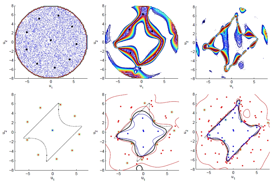
Figure 1: Illustration of the adaptive kriging technique (after Dubourg et al. (2011)). The original sample set is space-filling. In the later iterations, the sample points fall mainly within the margin of uncertainty defined by the kriging variance. Clustering is used in each step in order to select a few points to enrich the experimental design.

A limited number $K$ of new experimental points (to be added to $\mathfrak{X}$) is then obtained by clustering the large sample set and added to the experimental design. Convergence criteria are established based on the bounds on $P_{f}$ obtained by the boundaries of the margin $\mathfrak{M}$, see Dubourg et al. (2011) for details.

3.6 Conclusion

Quadratic response surfaces, polynomial chaos expansions and kriging techniques have been reviewed as meta-modelling techniques for structural reliability analysis. Whatever their respective advantages and drawbacks, all these meta-models are usually used as substitutes for the original limit state function, meaning that the probability of failure is simply evaluated as in Eq.(28). In principle there is no guarantee that the probability of failure evaluated on the surrogate is equal or sufficiently close to the that obtained from the surrogate. A way of addressing this issue is now proposed.

4 Meta-models as a means for importance sampling

4.1 Introduction

As shown in the previous sections meta-models are usually built in a first step of the reliability analysis and then substituted for the “true” limit state function. Even if some adaptive scheme allows one to ensure the closeness of the original function and its surrogate, the unbiasedness of the estimator of $P_{f}$ based on the surrogate cannot be guaranteed.

In order to solve this problem, Dubourg et al. (2011) propose to combine the well-known importance sampling technique with kriging in order to get unbiased estimates of the probability of failure. As shown below, the surrogate is used to build a “smart” importance sampling density instead of being substituted as in Eq.(28).

4.2 Reminder on importance sampling

The reason why crude Monte Carlo simulation is inefficient for evaluating probabilities of failure is that a typical sample will contain a majority of points located in the central part of the input distributions whereas the realizations that lead to failure are in the tails. The key idea of importance sampling is to use an instrumental density which allows one to concentrate the drawn samples in the region of interest. Consider a non zero probability density function $h(\boldsymbol{x})$ defined on $\textrm{I\!R}^{M}$. Eq.(3) may be recast as:

$$\begin{split}P_{f}&=\int_{\textrm{I\!R}^{M}}\boldsymbol{1}_{{\mathcal{D}}_{f}}(\boldsymbol{x})\,\frac{f_{\boldsymbol{X}}(\boldsymbol{x})}{h(\boldsymbol{x})}h(\boldsymbol{x})\,d\boldsymbol{x}\\ &={\textrm{I\!E}}_{h}\left[\boldsymbol{1}_{{\mathcal{D}}_{f}}(\boldsymbol{X})\frac{f_{\boldsymbol{X}}(\boldsymbol{X})}{h(\boldsymbol{X})}\right]\end{split}$$ (48)

where the subscript in ${\textrm{I\!E}}_{h}\left[\bullet\right]$ means that the expectation is taken with respect to the probability measure associated with $h$. The classical importance sampling (IS) estimator is built from a sample set drawn from the instrumental distribution, say $\mathfrak{X}_{h}=\left\{\boldsymbol{x}_{h}^{(i)},\;i=1,\,\dots\,,N\right\}$:

$$\hat{P}_{f,IS}\equiv\frac{1}{N}\sum_{i=1}^{N}\boldsymbol{1}_{{\mathcal{D}}_{f}}(\boldsymbol{x}^{(i)}_{h})\frac{f_{\boldsymbol{X}}(\boldsymbol{x}^{(i)}_{h})}{h(\boldsymbol{x}^{(i)}_{h})}$$ (49)

The art of importance sampling consists in using an instrumental density that minimizes the variance of the latter estimator. Rubinstein and Kroese (2008) shows that the optimal density (which actually reduces the variance of the estimator to 0) reads:

$$h^{*}(\boldsymbol{x})=\frac{\boldsymbol{1}_{{\mathcal{D}}_{f}}(\boldsymbol{X})\,f_{\boldsymbol{x}}(\boldsymbol{x})}{\int_{{\mathcal{D}}_{\boldsymbol{x}}}\boldsymbol{1}_{{\mathcal{D}}_{f}}(\boldsymbol{X})\,f_{\boldsymbol{X}}(\boldsymbol{x})}=\frac{\boldsymbol{1}_{{\mathcal{D}}_{f}}(\boldsymbol{x})\,f_{\boldsymbol{X}}(\boldsymbol{x})}{P_{f}}$$ (50)

However this density cannot be used in practice since it depends on the unknown quantity of interest $P_{f}$. The key idea of meta-model-based importance sampling (called meta-IS for short) is to surrogate this optimal instrumental density by kriging.

4.3 Sub-optimal instrumental density

Assuming that some kriging meta-model $\widehat{Y}$ of the limit state function is available, the indicator function of the failure domain may be replaced by the probabilistic classification function (see Eq.(45)) evaluated for $t=0$:

$$\pi(\boldsymbol{x})\equiv\Phi\left(\frac{0-\mu_{\widehat{Y}}\left(\boldsymbol{x}\right)}{\sigma_{\widehat{Y}}\left(\boldsymbol{x}\right)}\right)$$ (51)

Indeed if the surrogate is accurate in a given point $\boldsymbol{x}_{0}$ then $\sigma_{\widehat{Y}}(\boldsymbol{x}_{0})$ is close to zero and $\mu_{\widehat{Y}}(\boldsymbol{x}_{0})$ is close to $g(\boldsymbol{x}_{0})$. If the latter is negative then $\mu_{\widehat{Y}}(\boldsymbol{x}_{0})/\sigma_{\widehat{Y}}(\boldsymbol{x}_{0})\rightarrow-\infty$ and $\pi(\boldsymbol{x}_{0})\approx 0$. In contrast, if $g(\boldsymbol{x}_{0})>0$ then $\mu_{\widehat{Y}}(\boldsymbol{x}_{0})/\sigma_{\widehat{Y}}(\boldsymbol{x}_{0})\rightarrow+\infty$ and $\pi(\boldsymbol{x}_{0})\approx 1$. Thus $\pi(\boldsymbol{x})$ is a kind of “smoothed” version of the indicator function $\boldsymbol{1}_{{\mathcal{D}}_{f}}$. This leads to the meta-IS instrumental density (to be compared with Eq.(50)) :

$$\tilde{h}(\boldsymbol{x})\equiv\frac{\pi(\boldsymbol{x})\,f_{\boldsymbol{X}}(\boldsymbol{x})}{P_{f\varepsilon}}=\frac{\Phi\left(-\mu_{\widehat{Y}}(\boldsymbol{x})/\sigma_{\widehat{Y}}(\boldsymbol{x})\right)\,f_{\boldsymbol{X}}(\boldsymbol{x})}{P_{f\varepsilon}}$$ (52)

where the normalization constant $P_{f\varepsilon}$ reads:

$$P_{f\varepsilon}\equiv\int_{{\mathcal{D}}_{\boldsymbol{X}}}\Phi\left(-\mu_{\widehat{Y}}(\boldsymbol{x})/\sigma_{\widehat{Y}}(\boldsymbol{x})\right)\,f_{\boldsymbol{X}}(\boldsymbol{x})\,d\boldsymbol{x}$$ (53)

As an example the optimal instrumental density and that obtained from the above procedure is shown in Figure 2 where the quadratic limit state is taken from Der Kiureghian and Dakessian (1998).

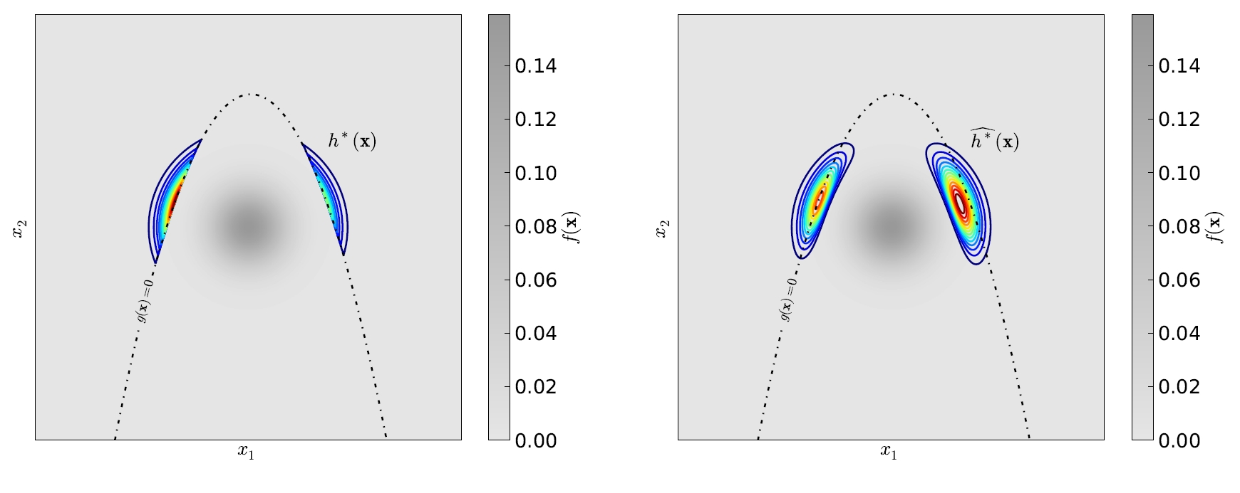
Figure 2: Comparison of the optimal (left) and the meta-IS (right) instrumental probability density functions (after Dubourg et al. (2011))

4.4 Meta-IS estimator of the probability of failure

Substituting for Eq.(52) in Eq.(48) and using Eq.(53) one gets:

$$P_{f}=\alpha_{corr}\,P_{f\varepsilon}$$ (54)

where:

$$\alpha_{corr}={\textrm{I\!E}}_{\tilde{h}}\left[\frac{\boldsymbol{1}_{{\mathcal{D}}_{f}}(\boldsymbol{X})}{\pi(\boldsymbol{X})}\right]$$ (55)

is a correction factor that quantifies the error that has been made by substituting the probabilistic classification function $\pi(\boldsymbol{x})$ to the indicator function $\boldsymbol{1}_{{\mathcal{D}}_{f}}(\boldsymbol{X})$. The Monte Carlo estimate of the latter then reads:

$$\begin{split}\widehat{P_{f}}_{metaIS}&=\widehat{\alpha}_{corr}\,\widehat{P_{f\varepsilon}}\\ \text{where:}\qquad\widehat{\alpha}_{corr}&={\frac{1}{N_{corr}}\sum_{k=1}^{N_{corr}}\frac{\boldsymbol{1}_{{\mathcal{D}}_{f}}(\tilde{\boldsymbol{x}}^{(k)})}{\pi(\tilde{\boldsymbol{x}}^{(k)})}}\\ \widehat{P_{f\varepsilon}}&={\frac{1}{N_{\varepsilon}}\sum_{l=1}^{N_{\varepsilon}}\pi(\boldsymbol{x}^{(l)})}\end{split}$$ (56)

In the above equation, the first sum is computed using $N_{corr}$ realizations following the meta-IS PDF $\tilde{h}$ while the second sum is computed using $N_{\varepsilon}$ realizations of $\boldsymbol{X}$.

The estimator in Eq.(56) is proven to be unbiased and its variance may be derived straightforwardly Dubourg et al. (2011). From a computational point of view, it is important to note that $\widehat{P_{f\varepsilon}}$ is evaluated at low cost since it only requires the evaluation of the probabilistic classification function Eq.(51) which is analytical when the kriging surrogate is available. Thus $N_{\varepsilon}=10^{5-6}$ is affordable, leading to an almost exact value of $P_{f\varepsilon}$. In contrast, computing $\widehat{\alpha}_{corr}$ requires the evaluation the “true” indicator function of the failure domain. Thus $N_{corr}$ shall be limited to a few hundredw in practice.

4.5 Meta-IS estimator of the probability of failure

As a conclusion, using meta-models as a tool for defining a quasi-optimal instrumental density for importance sampling solves the problem of possible biasedness resulting from a direct substitution. This is a great advantage of meta-IS compared to the approaches by Bichon et al. (2008); Echard et al. (2011).

In order to optimize the efficiency a trade-off between a) the number of calls to the $g$-function (say, $N$) required for building the meta-model $\widehat{Y}$ and b) the number of samples $N_{corr}$ shall be found, since the “total cost” is $N+N_{corr}$. A large $N$ will provide a very accurate meta-model that will lead to $\alpha_{corr}\approx 1$ at a high computational cost though. In contrast a “medium accurate” surrogate will be compensated for by a correction factor $\alpha_{corr}\neq 1$. In order to balance these two aspects a procedure based on cross-validation is proposed by Dubourg et al. (2011) for stopping the iterative improvement of the kriging surrogate (Section 3.5.3) when $P_{f\varepsilon}$ is sufficiently close to $P_{f}$.

5 Application examples

5.1 Frame structure - Polynomial chaos expansion (Blatman and Sudret, 2010a)

Let us consider a 3-span, 5-storey frame structure as the one sketched in Figure 3. Of interest is the top floor displacement when the structure is submitted to lateral loads. The associated serviceability limit state function reads:

$$g(\boldsymbol{X})\,=\,u_{max}-\text{{FEModel}}(\boldsymbol{X})$$ (57)

where $u_{max}$ is a given threshold, FEModel$(\bullet)$ is the finite element model (considered as a black box) that evaluates the top floor horizontal displacement, and $\boldsymbol{X}$ gathers 21 correlated random variables which describe the uncertainty in the member’s cross section, inertia and applied loads, see Blatman and Sudret (2010a) for the complete description. The probability of failure is investigated for different values of the threshold, namely $u_{max}=4-9$ cm. Reference values are obtained by FORM followed by importance sampling ($500,000$ model evaluations are used to get a coefficient of variation less than $1.0\%$ on $P_{f}$).

Figure 3: Sketch of a 3-span, 5-story frame structure subjected to lateral loads

Estimates of the reliability index are computed by post-processing a full third-order PC expansion as well as a sparse PC approximation. The latter is built up by setting the target approximation error equal to $10^{-3}$ (this is an overall mean square error that drives the convergence of the adaptive PC expansion, see the original paper for details). The estimates of the various generalized reliability indices $\beta=-\Phi^{-1}(P_{f})$ are reported in Table 5.1.

Frame structure - Estimates of the generalized reliability index $\beta=-\Phi^{-1}(P_{f})$ for various values of the threshold displacement   Threshold (cm)   Reference Full PCE Sparse PCE $\beta^{REF}$ $\widehat{\beta}$ $\epsilon\;(\%)$ $\widehat{\beta}$ $\epsilon\;(\%)$ 4 2.27 2.26 0.4 2.29 0.9 5 2.96 3.00 1.4 3.01 1.7 6 3.51 3.60 2.6 3.61 2.8 7 3.96 4.12 4.0 4.11 3.8 8 4.33 4.58 5.8 4.56 5.3 9 4.65 4.99 7.3 4.94 6.2 Relative error $1\cdot 10^{-3}$ $1\cdot 10^{-3}$ # terms in PCE 2,024 138 # FE runs 53,240 3,724 450

From the results in Table 5.1 it is seen that the sparse polynomial chaos expansion allows one to evaluate accurately reliability indices up to $\beta=4$ with less than 5% error. The parametric analysis w.r.t the threshold is obtained for free since the PC expansion is computed once and for all. As a whole the analysis has required 450 calls to the finite element model. Note that it also yields the statistical moments of the response as well as sensitivity results at the same cost (see Blatman and Sudret (2010b) for details).

It should be emphasized that PC expansions provide an approximation whose accuracy is controlled globally, i.e. in a least-square sense. It does not guarantee a perfect control of the accuracy in the tail of the distribution of the limit state function though. This means that this approach should not be used for very small probabilities. Results reported in the literature show that it is robust up to $P_{f}=10^{-4/-5}$.

5.2 System reliability - meta-IS (Dubourg, 2011)

As an illustration consider the following system limit state function (Waarts, 2000):

$$g(\boldsymbol{x})=\min\left(\begin{array}[c]{c}3+(x_{1}-x_{2})^{2}/10-(x_{1}+x_{2})/\sqrt{2}\\ 3+(x_{1}-x_{2})^{2}/10+(x_{1}+x_{2})/\sqrt{2}\\ x_{1}-x_{2}+7/\sqrt{2}\\ x_{2}-x_{1}+7/\sqrt{2}\end{array}\right)$$ (58)

where the two components of the input random vector $\boldsymbol{X}$ are independent standard normal variables.

Meta-importance sampling – system reliability analysis (after Dubourg (2011)) Monte Carlo Subset simulation Meta-IS Computational cost 172,000 284,195 40 + 200 $\hat{P}_{f}$ $2.26\;10^{-3}$ $2.28\;10^{-3}$ $2.38\;10^{-3}$ C.o.V $<$ 5% $<$3% $<$ 5%

The reference results are obtained by crude Monte Carlo simulation so as to obtain a coefficient of variation less than 5%. They are reported in Table 5.2 together with the results obtained by meta-importance sampling. It is shown that only 40 runs of the limit state function are required in order to build a sufficiently accurate surrogate. Then only 200 runs of the true model are required using the sub-optimal instrumental density in order to compute the probability of failure within 5% accuracy. The computational cost is thus decreased by two order of magnitude.

6 Conclusions

Meta-modelling techniques have become inescapable in modern engineering since they allow one to address real-world reliability problems at an affordable computational cost. In this paper, well-established reliability methods such as FOSM and FORM/SORM are reinterpreted as basic meta-models. More advanced techniques such as polynomial chaos expansions and kriging have been reviewed and show promising features in terms of performance and accuracy.

This paper also emphasizes the need for engineers to catch up with the latest technologies developed in computer science and applied mathematics (including statistics) in order to further innovate in their respective fields.

References

- Akaike (1973) Akaike, H. (1973). Information theory and maximum likelihood principles. In B. Petrov and F. Csaki (Eds.), Proc. 2nd Int. Symposium on information theory, Budapest, pp. 281–297.
- Au and Beck (1999) Au, S. and J. Beck (1999). A new adaptive importance sampling scheme for reliability calculations. Structural Safety 21(2), 135–158.
- Au and Beck (2001) Au, S. and J. Beck (2001). Estimation of small failure probabilities in high dimensions by subset simulation. Prob. Eng. Mech. 16(4), 263–277.
- Basudhar and Missoum (2008) Basudhar, A. and S. Missoum (2008). Adaptive explicit decision functions for probabilistic design and optimization using support vector machines. Computers & Structures 86(19-20), 1904–1917.
- Basudhar et al. (2008) Basudhar, A., S. Missoum, and A. Sanchez (2008). Limit state function identification using Support Vector Machines for discontinuous responses and disjoint failure domains. Prob. Eng. Mech 23, 1–11.
- Berveiller et al. (2004) Berveiller, M., B. Sudret, and M. Lemaire (2004). Presentation of two methods for computing the response coefficients in stochastic finite element analysis. In Proc. 9th ASCE Specialty Conference on Probabilistic Mechanics and Structural Reliability, Albuquerque, USA.
- Berveiller et al. (2006) Berveiller, M., B. Sudret, and M. Lemaire (2006). Stochastic finite elements: a non intrusive approach by regression. Eur. J. Comput. Mech. 15(1-3), 81–92.
- Bichon et al. (2008) Bichon, B., M. Eldred, L. Swiler, S. Mahadevan, and J. McFarland (2008). Efficient global reliability analysis for nonlinear implicit performance functions. AIAA Journal 46(10), 2459–2468.
- Bjerager (1988) Bjerager, P. (1988). Probability integration by directional simulation. J. Eng. Mech. 114(8), 1285–1302.
- Blatman (2009) Blatman, G. (2009). Adaptive sparse polynomial chaos expansions for uncertainty propagation and sensitivity analysis. Ph. D. thesis, Université Blaise Pascal, Clermont-Ferrand.
- Blatman and Sudret (2010a) Blatman, G. and B. Sudret (2010a). An adaptive algorithm to build up sparse polynomial chaos expansions for stochastic finite element analysis. Prob. Eng. Mech. 25(2), 183–197.
- Blatman and Sudret (2010b) Blatman, G. and B. Sudret (2010b). Efficient computation of global sensitivity indices using sparse polynomial chaos expansions. Reliab. Eng. Sys. Safety 95, 1216–1229.
- Blatman and Sudret (2011) Blatman, G. and B. Sudret (2011). Adaptive sparse polynomial chaos expansion based on Least Angle Regression. J. Comput. Phys. 230, 2345–2367.
- Bourinet et al. (2011) Bourinet, J.-M., F. Deheeger, and M. Lemaire (2011). Assessing small failure probabilities by combined subset simulation and support vector machines. Structural Safety 33(6), 343–353.
- Breitung (1984) Breitung, K. (1984). Asymptotic approximation for multinormal integrals. J. Eng. Mech. 110(3), 357–366.
- Breitung (1989) Breitung, K. (1989). Asymptotic approximations for probability integrals. Prob. Eng. Mech. 4(4), 187–190.
- Bucher and Bourgund (1990) Bucher, C. and U. Bourgund (1990). A fast and efficient response surface approach for structural reliability problems. Structural Safety 7, 57–66.
- Chilès and Delfiner (1999) Chilès, J.-P. and P. Delfiner (1999). Geostatistics: Modeling Spatial Uncertainty. Wiley, New York.
- Choi et al. (2004) Choi, S., R. Grandhi, and R. Canfield (2004). Structural reliability under non-Gaussian stochastic behavior. Computers & Structures 82, 1113–1121.
- Cornell (1969) Cornell, C.-A. (1969). A probability-based structural code. J. American Concrete Institute 66(12), 974–985.
- Cressie (1993) Cressie, N. (1993). Statistics for spatial data. John Wiley & Sons Inc.
- Das and Zheng (2000) Das, P.-K. and Y. Zheng (2000). Cumulative formation of response surface and its use in reliability analysis. Prob. Eng. Mech. 15(4), 309–315.
- Deheeger (2008) Deheeger, F. (2008). Couplage mécano-fiabiliste : SMART - méthodologie d’apprentissage stochastique en fiabilité. Ph. D. thesis, Université Blaise Pascal, Clermont-Ferrand.
- Deheeger and Lemaire (2007) Deheeger, F. and M. Lemaire (2007). Support vector machine for efficient subset simulations: 2smartmethod. In Proc. 10th Int. Conf. on Applications of Stat. and Prob. in Civil Engineering (ICASP10), Tokyo, Japan.
- Der Kiureghian and Dakessian (1998) Der Kiureghian, A. and T. Dakessian (1998). Multiple design points in first and second-order reliability. Structural Safety 20(1), 37–49.
- Der Kiureghian and de Stefano (1991) Der Kiureghian, A. and M. de Stefano (1991). Efficient algorithms for second order reliability analysis. J. Eng. Mech. 117(12), 2906–2923.
- Der Kiureghian et al. (1987) Der Kiureghian, A., H. Lin, and S. Hwang (1987). Second order reliability approximations. J. Eng. Mech. 113(8), 1208–1225.
- Ditlevsen and Madsen (1996) Ditlevsen, O. and H. Madsen (1996). Structural reliability methods. J. Wiley and Sons, Chichester.
- Ditlevsen et al. (1987) Ditlevsen, O., R. Olesen, and G. Mohr (1987). Solution of a class of load combination problems by directional simulation. Structural Safety 4, 95–109.
- Dubourg (2011) Dubourg, V. (2011). Adaptive surrogate models for reliability analysis and reliability-based design optimization. Ph. D. thesis, Universit Blaise Pascal – Clermont II.
- Dubourg et al. (2011) Dubourg, V., J.-M. Bourinet, B. Sudret, and M. Cazuguel (2011). Reliability-based design optimization of an imperfect submarine pressure hull. In M. Faber (Ed.), Proc. 11th Int. Conf. on Applications of Stat. and Prob. in Civil Engineering (ICASP11), Zurich, Switzerland.
- Dubourg et al. (2011) Dubourg, V., F. Deheeger, and B. Sudret (2011). Metamodel-based importance sampling for the estimation of rare event probabilities. Prob. Eng. Mech.. Submitted for publication.
- Dubourg et al. (2011) Dubourg, V., B. Sudret, and J.-M. Bourinet (2011). Reliability-based design optimization using kriging and subset simulation. Struct. Multidisc. Optim. 44(5), 673–690.
- Duprat and Sellier (2006) Duprat, F. and A. Sellier (2006). Probabilistic approach to corrosion risk due to carbonation via an adaptive response surface method. Prob. Eng. Mech. 21(3), 207–216.
- Echard et al. (2011) Echard, B., N. Gayton, and M. Lemaire (2011). AK-MCS: an active learning reliability method combining kriging and monte carlo simulation. Structural Safety 33(2), 145–154.
- Faravelli (1989) Faravelli, L. (1989). Response surface approach for reliability analysis. J. Eng. Mech. 115(12), 2763–2781.
- Gayton et al. (2003) Gayton, N., J. Bourinet, and M. Lemaire (2003). CQ2RS: a new statistical approach to the response surface method for reliability analysis. Structural Safety 25(1), 99–121.
- Ghanem and Spanos (1991) Ghanem, R. and P. Spanos (1991). Stochastic finite elements – A spectral approach. Springer Verlag. (Reedited by Dover Publications, 2003).
- Ghiocel and Ghanem (2002) Ghiocel, D. and R. Ghanem (2002). Stochastic finite element analysis of seismic soil-structure interaction. J. Eng. Mech. 128, 66–77.
- Hasofer and Lind (1974) Hasofer, A.-M. and N.-C. Lind (1974). Exact and invariant second moment code format. J. Eng. Mech. 100(1), 111–121.
- Hohenbichler et al. (1987) Hohenbichler, M., S. Gollwitzer, W. Kruse, and R. Rackwitz (1987). New light on first- and second order reliability methods. Structural Safety 4, 267–284.
- Hohenbichler and Rackwitz (1988) Hohenbichler, M. and R. Rackwitz (1988). Improvement of second-order reliability estimates by importance sampling. J. Eng. Mech. 114(12), 2195–2199.
- Hsu and Ching (2010) Hsu, W.-C. and J. Ching (2010). Evaluating small failure probabilities of multiple limit states by parallel subset simulation. Prob. Eng. Mech. 25(3), 291–304.
- Hurtado (2004a) Hurtado, J. (2004a). An examination of methods for approximating implicit limit state functions from the viewpoint of statistical learning theory. Structural Safety 26, 271–293.
- Hurtado (2004b) Hurtado, J. (2004b). Structural reliability – Statistical learning perspectives, Volume 17 of Lecture notes in applied and computational mechanics. Springer.
- Isukapalli (1999) Isukapalli, S. S. (1999). Uncertainty Analysis of Transport-Transformation Models. Ph. D. thesis, The State University of New Jersey.
- Jaynes (1982) Jaynes, E. (1982). On the rationale of maximum-entropy methods. Proc. IEEE 70(9), 939–952.
- Kapur and Kesavan (1992) Kapur, J. and H. Kesavan (1992). Entropy optimization principles with application. Academic Press, New York.
- Katafygiotis and Cheung (2005) Katafygiotis, L. and S. Cheung (2005). A two-stage subset simulation-based approach for calculating the reliability of inelastic structural systems subjected to Gaussian random excitations. Comput. Methods Appl. Mech. Engrg. 194(12-16), 1581–1595.
- Kaymaz (2005) Kaymaz, I. (2005). Application of kriging method to structural reliability problems. Structural Safety 27(2), 133–151.
- Keese and Matthies (2005) Keese, A. and H.-G. Matthies (2005). Hierarchical parallelisation for the solution of stochastic finite element equations. Computers & Structures 83, 1033–1047.
- Kim and Na (1997) Kim, S.-H. and S.-W. Na (1997). Response surface method using vector projected sampling points. Structural Safety 19(1), 3–19.
- Krige (1951) Krige, D. (1951). A statistical approach to some basic mine valuation problems on the Witwatersrand. J. of the Chem., Metal. and Mining Soc. of South Africa 52(6), 119–139.
- Le Maître et al. (2002) Le Maître, O., M. Reagan, H. Najm, R. Ghanem, and O. Knio (2002). A stochastic projection method for fluid flow – II. Random process. J. Comput. Phys. 181, 9–44.
- Leira et al. (2005) Leira, B., T. Holm s, and K. Herfjord (2005). Application of response surfaces for reliability analysis of marine structures. Reliab. Eng. Sys. Safety 90(2-3), 131–139.
- Lemaire (1998) Lemaire, M. (1998). Finite element and reliability : combined methods by response surfaces. In G. Frantziskonis (Ed.), Probamat-21st Century, Probabilities and Materials : Tests, Models and Applications for the 21st century, pp. 317–331. Kluwer Academic Publishers.
- Lemaire (2009) Lemaire, M. (2009). Structural reliability. Wiley.
- Maes et al. (1993) Maes, M., K. Breitung, and D. Dupuis (1993). Asymptotic importance sampling. Structural Safety 12, 167–183.
- Marrel et al. (2008) Marrel, A., B. Iooss, F. Van Dorpe, and E. Volkova (2008). An efficient methodology for modeling complex computer codes with Gaussian processes. Comput. Stat. Data Anal. 52, 4731–4744.
- Matheron (1963) Matheron, G. (1963). Principles of geostatistics. Economic Geology 58, 1246–1266.
- McKay et al. (1979) McKay, M. D., R. J. Beckman, and W. J. Conover (1979). A comparison of three methods for selecting values of input variables in the analysis of output from a computer code. Technometrics 2, 239–245.
- Melchers (1990) Melchers, R. (1990). Radial importance sampling for structural reliability. J. Eng. Mech. 116, 189–203.
- Melchers (1999) Melchers, R.-E. (1999). Structural reliability analysis and prediction. John Wiley & Sons.
- Neal (2003) Neal, R. (2003). Slice sampling. Annals Stat. 31, 705–767.
- Pendola et al. (2000) Pendola, M., A. Mohamed, M. Lemaire, and P. Hornet (2000). Combination of finite element and reliability methods in nonlinear fracture mechanics. Reliability Engineering & System Safety 70(1), 15–27.
- Pradlwarter et al. (2007) Pradlwarter, H., G. Schuëller, P. Koutsourelakis, and D. Charmpis (2007). Application of line sampling simulation method to reliability benchmark problems. Structural Safety 29(3), 208–221.
- Rackwitz and Fiessler (1978) Rackwitz, R. and B. Fiessler (1978). Structural reliability under combined load sequences. Computers & Structures 9, 489–494.
- Rajashekhar and Ellingwood (1993) Rajashekhar, M.-R. and B.-R. Ellingwood (1993). A new look at the response surface approach for reliability analysis. Structural Safety 12, 205–220.
- Romero et al. (2004) Romero, V., L. Swiler, and A. Giunta (2004). Construction of response surfaces based on progressive lattice-sampling experimental designs with application to uncertainty propagation. Structural Safety 26(2), 201–219.
- Rubinstein and Kroese (2008) Rubinstein, R. and D. Kroese (2008). Simulation and the Monte Carlo method. Wiley Series in Probability and Statistics. Wiley.
- Sacks et al. (1989) Sacks, J., W. Welch, T. Mitchell, and H. Wynn (1989). Design and analysis of computer experiments. Stat. Sci. 4, 409–435.
- Santner et al. (2003) Santner, T., B. Williams, and W. Notz (2003). The Design and Analysis of Computer Experiments. Springer, New York.
- Schwartz (1978) Schwartz, G. (1978). Estimating the dimension of a model. Annals Stat. 6(2), 461–464.
- Soize and Ghanem (2004) Soize, C. and R. Ghanem (2004). Physical systems with random uncertainties: chaos representations with arbitrary probability measure. SIAM J. Sci. Comput. 26(2), 395–410.
- Stone (1974) Stone, M. (1974). Cross-validatory choice and assessment of statistical predictions. J. Royal Stat. Soc., Series B 36, 111–147.
- Stuart et al. (1999) Stuart, A., K. Ord, and S. Arnold (1999). Kendall’s advanced theory of statistics Vol. 2A – Classical inference and the linear model (6th ed.). Arnold.
- Sudret (2007) Sudret, B. (2007). Uncertainty propagation and sensitivity analysis in mechanical models – Contributions to structural reliability and stochastic spectral methods. Université Blaise Pascal, Clermont-Ferrand, France. Habilitation à diriger des recherches, 173 pages.
- Sudret (2008) Sudret, B. (2008). Global sensitivity analysis using polynomial chaos expansions. Reliab. Eng. Sys. Safety 93, 964–979. In press.
- Sudret et al. (2003) Sudret, B., M. Berveiller, and M. Lemaire (2003). Application of a stochastic finite element procedure to reliability analysis. In M. Maes and L. Huyse (Eds.), Proc 11th IFIP WG7.5 Conference on Reliability and Optimization of Structural Systems, Banff, Canada, pp. 319–327. Balkema, Rotterdam.
- Sudret et al. (2011) Sudret, B., G. Blatman, and M. Berveiller (2011). Response surfaces based on polynomial chaos expansions, Chapter 8, pp. 147–168. Construction reliability – safety, variability and sustainability (J. Baroth, F. Schoefs, and D. Breysse (Eds)). ISTE/Wiley.
- Sudret and Der Kiureghian (2000) Sudret, B. and A. Der Kiureghian (2000). Stochastic finite elements and reliability: a state-of-the-art report. Technical Report UCB/SEMM-2000/08, University of California, Berkeley. 173 pages.
- Sudret and Der Kiureghian (2002) Sudret, B. and A. Der Kiureghian (2002). Comparison of finite element reliability methods. Prob. Eng. Mech. 17, 337–348.
- Vrouwenvelder (1997) Vrouwenvelder, T. (1997). The JCSS probabilistic model code. Structural Safety 19(3), 245–251.
- Waarts (2000) Waarts, P.-H. (2000). Structural reliability using finite element methods: an appraisal of DARS: Directional Adaptive Response Surface Sampling. Ph. D. thesis, Technical University of Delft, The Netherlands.
- Xiu (2009) Xiu, D. (2009). Fast numerical methods for stochastic computations: a review. Comm. Comput. Phys. 5(2-4), 242–272.
- Xiu and Hesthaven (2005) Xiu, D. and J. Hesthaven (2005). High-order collocation methods for differential equations with random inputs. SIAM J. Sci. Comput. 27(3), 1118–1139.
- Xiu and Karniadakis (2002) Xiu, D. and G. Karniadakis (2002). The Wiener-Askey polynomial chaos for stochastic differential equations. SIAM J. Sci. Comput. 24(2), 619–644.