X-ray spectral curvature of High Frequency Peaked BL Lacs:
a predictor for the TeV flux

Abstract

Most of the extragalactic sources detected at TeV energies are BL Lac objects. They belong to the subclass of “high frequency peaked BL Lacs” (HBLs) exhibiting spectral energy distributions with a lower energy peak in the X-ray band; this is widely interpreted as synchrotron emission from relativistic electrons. The X-ray spectra are generally curved, and well described in terms of a log-parabolic shape. In a previous investigation of TeV HBLs (TBLs) we found two correlations between their spectral parameters. (1) The synchrotron peak luminosity $L_{p}$ increases with its peak energy $E_{p}$; (2) the curvature parameter $b$ decreases as $E_{p}$ increases. The first is consistent with the synchrotron scenario, while the second is expected from statistical/stochastic acceleration mechanisms for the emitting electrons. Here we present an extensive X-ray analysis of a sample of HBLs observed with XMM-Newton and Swift but undetected at TeV energies (UBLs), to compare their spectral behavior with that of TBLs. Investigating the distributions of their spectral parameters and comparing the TBL X-ray spectra with that of UBLs, we develop a criterion to select the best HBLs candidates for future TeV observations.

1 Introduction

The great majority ($\geq$ 80%) of the extragalactic sources detected to April 2011 in $\gamma$ rays at TeV energies are BL Lac objects. These are a class of active galactic nuclei (AGNs) characterized by strong and highly variable non-thermal radiations from radio frequencies to TeV energies. Their observational properties include weak or absent emission lines, two-hump shaped spectral energy distributions (SEDs, i.e., log $\nu F_{\nu}$ $vs$ log $\nu$), high radio and optical polarization, and superluminal motions. These are interpreted as the result of radiation from a relativistic jet closely aligned to the line of sight (Blandford & Rees, 1978).

BL Lacs come in two flavors: the “high-frequency peaked BL Lacs” (HBLs) in which the low energy component of the SED peaks between the UV band and X-rays, and the “low-frequency peaked BL Lacs” (LBLs) when the SED peak falls in the IR-optical range (Padovani & Giommi, 1995). It is widely agreed that this low-energy component is produced by synchrotron radiation of ultrarelativistic particles (i.e., electrons) accelerated in the jets, while the high energy component is likely due to inverse-Compton scattering of the synchrotron photons by the same electron population (Synchrotron Self-Compton, SSC, see e.g. Marscher & Gear 1985; Inoue & Takahara 1996).

In the following, we distinguish the HBLs detected at TeV energies from those not yet detected; we refer to the former as TBLs, and to the latter as UBLs.

A useful phenomenological description of the BL Lac X-ray spectra was introduced by Landau et al. (1986) in terms of a log-parabolic (LP) model (i.e., a parabolic shape in a double-log plot); subsequently, this model has been frequently adopted for the low energy bump, e.g., by Tanihata et al. (2004), Massaro et al. (2004) and other authors. Recently, the high energy component at TeV energies has also been successfully modeled with the same spectral shape (Massaro et al., 2006; Aharonian et al., 2009; Aleksic et al., 2011; acciari11; Abdo et al., 2011). We note that such LP synchrotron spectra are emitted by log-parabolic particle energy distributions (PEDs), obtained via the Fokker-Planck equation from a mono-energetic electron injection subjected to systematic and stochastic accelerations (Kardashev, 1962; Massaro et al., 2006; Stawarz & Petrosian, 2008; Paggi et al., 2009).

The LP model has been used also to describe the SED of other classes of jet-dominated sources: plerions (Campana et al., 2009), high frequency peaked (HFPs) radio sources (Maselli & Massaro, 2009), and, recently, Solar Flares(Grigis & Benz, 2008) and Gamma-Ray Bursts (GRBs) (Massaro et al., 2010a, 2011a).

Adopting the LP model, the X-ray SED of HBLs is described in terms of 3 parameters: (1) the peak energy, $E_{p}$, in $\nu F_{\nu}$ space, (2) the maximum height of the SED, $S_{p}$, evaluated at $E_{p}$ (or the corresponding peak luminosity $L_{p}$ $\simeq$ $4\pi D^{2}_{L}S_{p}$, with $D_{L}$ being the luminosity distance), and (3) the spectral curvature, $b$, around $E_{p}$ (Tramacere et al. 2007, Massaro et al. 2008a, hereafter M08).

Extensive investigations of the TBLs, based on all the X-ray observations available in the BeppoSAX, XMM-Newton and Swift archives between 1997 and 2007, have shown that several TBLs trace two correlations in the ($E_{p},L_{p},b$) parameter space: (1) the peak luminosity $L_{p}$ increases with $E_{p}$, as expected in the synchrotron scenario, (2) the curvature parameter $b$ decreases as $E_{p}$ increases (M08) as expected in a stochastic acceleration scenario (e.g., Tramacere et al. 2007).

As a result, TBLs cover a well-constrained region in the $E_{p}-b$ plane (hereinafter the “acceleration plane”). The correlation between $b$ and $E_{p}$ is evident for the 16 TBLs in M08, whilst no clear trend in the $E_{p}-L_{p}$ plane has been found for the whole sample.

Many HBLs have been targeted at TeV energies by HESS, Magic and VERITAS, but by no means all of them have been detected. It is striking that 19 out of 24 TBLs (to 2010, August 1st) belong to the Einstein Slew Survey Sample of BL Lacertae Objects (1ES, Elvis et al. 1992; Perlman et al. 1996), which includes only the brightest X-ray extragalactic sources at $\sim$ 1 keV. The remaining TBLs belong to three different samples, namely: 1) The ROSAT All-Sky Survey-Green Bank BL Lac catalog (RGB, Laurent-Muehleisen et al. 1999); 2) The sedentary survey of extreme high energy peaked BL Lacs (SHBL, Giommi et al. 2005); 3) The Hubble Space Telescope Survey of BL Lacertae Objects; (HST, Scarpa et al. 1999; Urry et al. 2000) (see Table 1). Consequently, we selected all the UBLs in the above four samples to search for possible differences between these sources and the TBLs.

In this paper, we present the sample selection criteria, the data reduction and data analysis procedures adopted to perform our investigation. Finally, comparing the distribution of the X-ray spectral parameters, we define criteria to predict future TBLs on the basis of X-ray observations only. The theoretical aspects and the interpretation of the observational results will be presented in Massaro et al. (2011b).

We use cgs units unless stated otherwise and we assume a flat cosmology with $H_{0}=72$ km s^-1 Mpc^-1, $\Omega_{M}=0.26$ and $\Omega_{\Lambda}=0.74$ (Dunkley, 2009).

2 Sample selection

We chose all the sources classified as BL Lac objects or BL Lac candidates in the ROMA BZCAT (Massaro et al., 2009, 2010b) that are present in the four samples in which TBLs are found (see Section 1), excluding the TBLs.

To compare the behavior of TBLs and UBLs, we selected a sample of UBLs on adopting the following criteria.

• We calculated the ratio $\Phi_{XR}$ between the X-ray flux $F_{X}$ (0.1 - 2.4 keV) and the radio flux $S_{1.4}$ (at 1.4 GHz), $\Phi_{XR}$ (i.e., $\Phi_{XR}=10^{-3}\,F_{X}/(S_{1.4}\,\Delta\nu)$ erg cm^-2 s^-1Jy^-1 with $\Delta\nu$ = 1GHz), using the values of $F_{X}$ and $S_{1.4}$ reported in the ROMA BZCAT (Massaro et al., 2009, 2010b). We select BL Lacs with $\Phi_{XR}$ $\geq$ 0.1 that corresponds to HBLs, according to the criterion established by Maselli & Massaro (2009).

• We restricted our sample to those sources with redshift $z\leq 0.539$, the highest redshift for an extragalactic TeV source (i.e., 3C 279, see Albert et al. 2008). Using this cut in redshift, we assumed that any extragalactic source with $z\geq 0.539$ could not be detected at TeV energies, because of the absorption by the extragalactic background light (Dwek & Krennrich, 2005).

• We considered only UBLs with X-ray observations, up to the end of October 2010, in the XMM-Newton or Swift archives, as performed for the TBLs by M08 that have an exposure longer than 150 s, in order to have a good chance of detection and a sufficient number of counts to perform the X-ray spectral analysis (see also M08).

There are 118 UBLs with known redshift. in the four samples considered. However, 71 UBLs are excluded by requiring $\Phi_{XR}\geq 0.1$, $z\leq$ 0.539 and with X-ray observations with exposure longer than 150 s. The remaining 47 UBLs constitute the sample we analyze below.

These 47 UBLs a total of 135 X-ray observations: 123 Swift observations and 12 by XMM-Newton. Only 19 UBLs out of the total 47 selected targets have been detected by Fermi during the first year of operations (Abdo et al., 2010).

Table 1: The properties of the BL Lac samples.

(1)	(2)	(3)	(4)	(5)	(6)
Sample	zmax	Total	TBLs	HBLs	UBLs
1ES	0.940	55	18	46	7
HST	0.940	94	19	57	3
SHBL	0.702	122	9	122	29
RGB	0.664	109	7	70	7

Col.(2) Total number of BL Lacs in the sample. Col.(3) Highest redshift in the sample. Col.(4) Number of TBLs present in the sample. Col.(5) Number of HBLs in the sample. Col.(6) Number of UBLs selected.

Table 1 reports: the highest redshift for the sample (Col. 2), the number of BL Lacs identified in the ROMA BZCAT (Col. 3), the number of TBLs in the sample (Col. 4), the number of HBLs present (Col. 5) and the UBLs selected according to the criteria defined above (Col. 6).

The basic data for all the 47 selected UBLs are reported in Table 2: the ROMA BZCAT name (Col. 1) and sample name (Col. 2), the equatorial coordinates (J2000) (Col. 3 and Col. 4), the redshift (Col. 5, from Massaro et al. 2010b), the luminosity distance $D_{L}$ (Col. 6), the value of the Galactic column density $N_{H,Gal}$ (Col. 7, see Kalberla et al. 2005), the X-ray to radio flux ratio $\Phi_{XR}$ (Col. 8) and the number of both the XMM-Newton and Swift observations (Col. 9 and Col. 10 respectively). Finally, in Col. (11) we show the TeV candidate class provided by our investigation discussed in Section 6.

Table 2: UBLs selected.

(1)	(2)	(3)	(4)	(5)	(6)	(7)	(8)	(9)	(10)	(11)	(12)
BZCAT Name	Other Name	RA	DEC	z	DL	NH,Gal	$\Phi_{XR}$	Swift	XMM	Fermi	TeV
		(J2000)	(J2000)		[Mpc]	$[10^{20}cm^{-2}]$					class
BZB J0013-1854	1RXS J001356.6-18540	00 13 56.0	-18 54 06.0	0.094	420.1	2.13	2.24	4	—	—	3
BZB J0123+3420	1ES 0120+340	01 23 08.5	+34 20 47.0	0.272	1359.7	5.20	5.74	17	1	—	3
BZB J0201+0034	1ES 0158+003	02 01 06.1	+00 34 00.0	0.298	1511.2	2.23	2.71	1	—	—	-
BZB J0208+3523	1RXS J020837.5+35231	02 08 38.2	+35 23 13.0	0.318	1629.9	6.27	5.76	—	2	y	2
BZB J0214+5144	RGB J0214+517	02 14 17.8	+51 44 52.0	0.049	212.0	14.4	0.16	3	—	—	3
BZB J0227+0202	1RXS J022716.6+02015	02 27 16.5	+02 02 00.0	0.456	2499.3	2.67	5.05	2	—	—	-
BZB J0325-1646	1RXS J032540.8-16460	03 25 41.1	-16 46 14.9	0.291	1470.1	3.27	10.1	3	—	y	-
BZB J0326+0225	1ES 0323+022	03 26 13.9	+02 25 14.0	0.147	681.2	7.87	1.77	3	1	y	1
BZB J0441+1504	1RXS J041112.1-39413	04 41 27.4	+15 04 54.0	0.109	492.3	14.0	7.28	1	1	—	-
BZB J0442-0018	1RXS J044229.8-00182	04 42 29.8	-00 18 34.9	0.449	2453.2	4.83	3.35	4	—	y	1
BZB J0621-3411	1RXS J062150.0-34114	06 21 49.4	-34 11 53.9	0.529	2991.5	4.08	2.30	1	—	—	-
BZB J0744+7433	1ES 0737+746	07 44 05.2	+74 33 56.9	0.314	1606.0	3.28	2.74	—	2	y	1
BZB J0751+1730	1RXS J075124.3+17304	07 51 25.0	+17 30 51.0	0.185	878.4	4.93	1.78	1	—	—	-
BZB J0753+2921	1RXS J075322.4+29215	07 53 24.6	+29 21 31.0	0.161	752.9	3.44	0.28	1	—	—	-
BZB J0847+1133	1RXS J084713.3+11334	08 47 12.8	+11 33 50.0	0.199	953.2	3.17	3.34	1	—	y	-
BZB J0916+5238	RGB J0916+526	09 16 51.8	+52 38 27.9	0.190	905.0	1.43	0.53	1	—	—	-
BZB J0930+4950	1RXS J093037.1+49502	09 30 37.5	+49 50 25.0	0.187	889.1	1.38	7.94	1	—	—	-
BZB J0952+7502	1RXS J095225.8+75021	09 52 24.1	+75 02 12.9	0.179	846.8	2.23	2.07	2	—	—	-
BZB J1010-3119	1RXS J101015.9-31190	10 10 15.9	-31 19 08.0	0.143	660.9	8.48	1.37	2	—	—	3
BZB J1022+5124	1RXS J102212.5+51240	10 22 12.6	+51 23 59.9	0.142	655.9	1.02	6.88	1	—	—	-
BZB J1053+4929	RGB J1053+494	10 53 44.0	+49 29 56.0	0.140	645.8	1.50	0.13	1	—	y	-
BZB J1056+0252	1RXS J105607.0+02521	10 56 06.6	+02 52 13.0	0.236	1155.7	3.82	17.3	1	—	—	-
BZB J1111+3452	1RXS J111131.2+34521	11 11 30.7	+34 52 02.9	0.212	1023.5	1.64	5.71	1	—	—	-
BZB J1117+2014	1RXS J111706.3+20141	11 17 06.1	+20 14 08.0	0.139	640.7	1.35	3.26	1	—	y	-
BZB J1136+6737	1136+676	11 36 29.9	+67 37 04.0	0.136	625.7	1.09	3.28	5	—	y	2
BZB J1145-0340	1RXS J114535.8-03394	11 45 35.1	-03 40 00.9	0.167	784.0	2.22	2.28	2	—	—	-
BZB J1154-0010	1RXS J115404.9-00100	11 54 04.5	-00 10 09.0	0.254	1256.9	2.06	2.75	1	—	—	-
BZB J1231+6414	1229+643	12 31 31.3	+64 14 17.9	0.163	763.3	2.12	0.43	—	1	—	-
BZB J1237+6258	1RXS J123739.2+62584	12 37 38.9	+62 58 41.9	0.297	1505.3	0.97	1.90	13	2	—	-
BZB J1253-3931	1RXS J125341.2-39320	12 53 41.2	-39 31 59.0	0.179	846.8	7.66	1.47	1	—	—	3
BZB J1257+2412	1ES 1255+244	12 57 31.9	+24 12 39.9	0.141	650.8	1.25	5.16	1	1	—	-
BZB J1341+3959	RGB J1341+399	13 41 05.1	+39 59 44.9	0.172	810.0	0.80	1.26	4	—	y	-
BZB J1417+2543	1RXS J141756.8+25432	14 17 56.5	+25 43 26.0	0.237	1161.3	1.54	1.72	5	—	y	2
BZB J1439+3932	1RXS J143917.7+39324	14 39 17.5	+39 32 42.0	0.344	1787.1	1.14	2.64	2	—	y	-
BZB J1442+1200	1ES 1440+122	14 42 48.1	+12 00 39.9	0.163	763.3	1.58	1.13	4	—	y	2
BZB J1510+3335	1RXS J151040.8+33351	15 10 41.1	+33 35 04.0	0.114	516.7	1.54	3.16	—	1	—	-
BZB J1534+3715	RGB J1534+372	15 34 47.2	+37 15 54.0	0.143	660.9	1.33	0.10	1	—	—	-
BZB J1605+5421	1RXS J160518.5+54210	16 05 19.0	+54 21 00.0	0.212	1023.5	0.89	5.53	1	—	—	-
BZB J1626+3513	RGB J1626+352	16 26 25.8	+35 13 41.0	0.497	2773.1	1.36	0.35	—	2	—	-
BZB J1728+5013	1728+502	17 28 18.5	+50 13 09.9	0.055	239.0	2.35	1.01	4	—	y	2
BZB J1743+1935	1ES 1741+196	17 43 57.7	+19 35 08.9	0.080	354.0	7.36	0.14	3	—	y	1
BZB J2131-0915	1RXS J213135.5-09152	21 31 35.3	-09 15 21.9	0.449	2453.2	3.62	1.74	1	—	y	-
BZB J2201-1707	1RXS J220156.0-17065	22 01 55.8	-17 07 00.0	0.169	794.4	2.91	5.92	2	—	—	-
BZB J2250+3824	RGB J2250+384	22 50 05.7	+38 24 37.0	0.119	541.2	10.4	0.24	16	—	y	2
BZB J2308-2219	1RXS J230846.7-22195	23 08 46.8	-22 19 49.0	0.137	630.7	1.86	7.12	1	—	—	-
BZB J2322+3436	RGB J2322+346	23 22 43.9	+34 36 14.0	0.098	439.3	6.83	0.11	2	—	y	-
BZB J2343+3439	1RXS J234332.5+34395	23 43 33.5	+34 39 48.9	0.366	1922.6	6.75	1.60	2	—	y	-

Col. (1) ROMA BZCAT source names. Col. (2) the name in the selected sample. Cols.(3,4) the right ascension and declination, respectively. Col. (4) gives the redshift (from ROMA BZCAT). Col. (5) reports the luminosity distance. Cols. (6) the Galactic column density along the line of sight (Kalberla et al., 2005). Col. (8) the X-ray to radio flux ratio $\Phi_{XR}$ (see Section 2). Cols. (9,10) report the number of X-ray observations per satellite. Col. (11) indicates if the source has been detected in the Fermi LAT 1st year catalog, wile Col. (12) the TeV candidate class derived from our analysis (see Section 6)

3 Data reduction procedures

The reduction procedure for the XMM-Newton data follows that described in Tramacere et al. (2007); additional details on both the XMM-Newton and Swift data reduction procedures can be found in M08 and Massaro et al. (2008b). In the following subsections we report only the basic details.

3.1 XMM-Newton observations

The sources were observed with XMM-Newton by means of all EPIC CCD cameras: the EPIC-PN (Struder et al., 2001), and EPIC-MOS (Turner et al., 2001).

Extractions of light curves, source and background spectra were done with the XMM-Newton  Science Analysis System (SAS) v6.5.0. The Calibration Index File (CIF) and the summary file of the Observation Data File (ODF) were generated using Updated Calibration Files (CCF) following the “User’s Guide to the XMM-Newton  Science Analysis System” (issue 3.1, Loiseau et al. 2004) and “The XMM-Newton  ABC Guide” (vers. 2.01, Snowden et al. 2004). Event files were produced by the EMCHAIN pipeline.

Light curves for each dataset were extracted, and all high-background intervals filtered out to exclude time intervals contaminated by solar flares. Then, by visual inspection, we selected good time intervals (GTI) far from solar flare peaks that have no count rate variations on time scales shorter than 500 seconds. Photons are extracted from an annular region using different apertures to minimize pile-up, which affects MOS data. The mean value of the external radius used for the annular region is $40$ $\prime\prime$.

A slightly restricted energy range (0.5–10 keV) is used to minimize residual calibration uncertainties. To ensure the validity of Gaussian statistics, data have been grouped by combining instrumental channels so that each bin contains 30 counts or more.

Figure 1: An example of the XMM-Newton spectrum of BZB J0208+3523 performed on Feb. 14, 2001 (Obs. ID 0084140101) is here reported to show the goodness of the fitting procedure with the LP model relative to the standard power-law. Left: the systematic deviations on both sides of the residuals from a best fit power-law with fixed $N_{H,Gal}$ show the need of intrinsic curvature. Right: the deviations disappear on using the LP model with fixed $N_{H,Gal}$.

3.2 Swift observations

The XRT data analysis was performed with the XRTDAS software (v. 2.1), developed at the ASI Science Data Center (ASDC) and included in the HEAsoft package (v. 6.0.2). Event files were calibrated and cleaned with standard filtering criteria using the xrtpipeline task.

Events in the energy range 0.3–10 keV with grades 0–12 (photon counting mode, PC) and 0–2 (windowed timing mode, WT) are used in the analyses; we refer to Hill et al. (2004) for a description of readout modes, and to Burrows et al. (2005) for a definition of XRT event grades. This slightly broader band than for XMM-Newton has no effect on the spectral fits (see M08). For the WT mode data, events were selected for temporal and spectral analysis using a 40 pixel wide (1 pixel $=2.36$ $"$) rectangular region centered on the source, and aligned along the WT one dimensional stream in sky coordinates. Background events were extracted from a nearby source-free rectangular region of 40 x 20 pixels.

For PC mode data, when the source count rate is above 0.45 counts s^-1, the data are significantly affected by pile-up in the inner part of the point spread function (Moretti et al., 2005). To remove the pile-up contamination, we extract only events contained in an annular region centered on the source (e.g., Perri et al. 2007). The inner radius of the region was determined by comparing the observed profiles with the analytical model derived by Moretti et al. (2005), and typically has a 4 or 5 pixels radius, while the outer radius is 20 pixels for each observation.

For Swift observations in which the source count rate was below the pile-up limit, events are instead extracted using a 20 pixel radius circle. The background for PC mode is estimated from a nearby source-free circular region of 20 pixel radius.

As for XMM-Newton, source spectra are binned to ensure a minimum of 30 counts per bin in order to ensure the validity of $\chi^{2}$ statistics.

4 X-ray Spectral analysis

We performed our spectral analysis primarily with the Sherpa modeling and fitting application (Freeman et al., 2001) and we used the xspec software package, version 11.3.2 (Arnaud, 1996) as a check of our results.

We describe the X-ray continuum with different spectral models: 1) an absorbed power-law with column density either free, or fixed at the Galactic value $N_{H,Gal}$; 2) an LP model; 3) a power-law with an exponential cutoff (PEC) adopting the new expression described below. In all models with fixed Galactic column density, we use $N_{H,Gal}$ values from the LAB survey (Kalberla et al., 2005) reported in Table 2.

The LP model in the form:

$$F(E)=K~{}E^{-a-b~{}log(E)}~{},$$ (1)

and the equivalent SED representation used by Tramacere et al. (2007) and M08 expressed as:

$$F(E)=\frac{S_{p}}{E^{2}}~{}{\left(\frac{E}{E_{p}}\right)}^{-b~{}log(E/E_{p})}~{},$$ (2)

with $S_{p}=E_{p}^{2}\,F(E_{p})$. Both these representations are in units of $photons~{}cm^{-2}~{}s^{-1}~{}keV^{-1}$. In particular, on using Equation 2, the values of the parameters $E_{p}$ (the SED energy peak), $S_{p}$ (the SED peak height at $E_{p}$), and $b$ (the curvature parameter) can be evaluated independently in the fitting procedure (Massaro et al., 2006; Tramacere et al., 2007).

We used the following expression to define the PEC model:

$$F(E)=\frac{\Sigma_{p}}{\epsilon_{p}^{2}}\left(\frac{E}{\epsilon_{p}}\right)^{\alpha}exp\left[\left(1-\frac{E}{\epsilon_{p}}\right)(2-\alpha)\right]~{}~{}~{}.$$ (3)

With Equation 3, the three parameters: $\epsilon_{p}$(the SED energy peak), $\Sigma_{p}$ (the SED height at the peak energy) and the photon index, $\alpha$, can be evaluated independently in the fitting procedure. We emphasize that the independent estimates of spectral parameters in both LP and PEC models performed by Equation 2 and Equation 3, allow us to investigate possible correlations among those parameters without the introduction of functional biases.

The results of the LP fits are reported in Appendix; the statistical uncertainties quoted refer to the 68% confidence level (one Gaussian standard deviation).

In some cases, a combination of poor statistics (due to short observational exposures or low count rate), restricted instrumental energy range, or the location of $E_{p}$ outside the observational energy range, make it difficult to evaluate the spectral curvature. In all these cases the single power-law model is an acceptable description of the X-ray spectra.

For 31 out of the remaining 107 (29%) of the complete sample of X-ray observations the spectral curvature is consistent with zero within 1$\sigma$. For 28 out of 135 observations the number of counts did not allow us to perform a good spectral analysis. In these 59 observations, we added together several low S/N observations for each sources (see the Appendix), and found that the co-added spectra are significantly curved in all cases.

5 Results

5.1 X-ray spectral properties

We present below the results of our X-ray spectral analysis performed on the UBL sample, and compare them with the known X-ray spectral behavior of TBLs (see M08).

We excluded the case of PKS 2155-204 from the TBL sample, because on several occasions this source has shown a high energy component dominating over the low energy one (e.g., Aharonian et al. (2009); Abdo et al. (2011); acciari11), making PKS 2155-204 more similar to a flat spectrum radio quasar than to a HBL.

We also excluded Mrk 421, because it has at least ten times the number of X-ray observations than any other TBL, and so could dominate the parameter distributions.

Finally, we excluded from our analysis the giant flare of Mrk 501 in 1997 (Massaro et al., 2006) and that of 1H 1426+428 (M08), because we are interested in investigating the spectral behavior in long-term quiescent states, rather than in rare, giant, flaring episodes.

We then compared all the UBLs and TBLs observations to search for possible differences in their X-ray spectral behavior that could lead to a possible criterion to identify TBL candidates.

Our results are summarized as follows:

1. Spectral models. We find that the absorbed power-law model gave unacceptable values of $\chi^{2}_{r}$ (i.e., $\chi^{2}_{r}\geq 1.5$) in all cases with sufficient statistics, for which the spectral curvature $b$ could be estimated, even when the intrinsic low energy absorption is left as a free parameter. This model is also inadequate to describe the high energy tail of the X-ray spectra above $\sim$ 4 keV (see Figure 1 left panel).

Such a lack of intrinsic absorption agrees with the X-ray spectral analyses of TBLs, that are featureless over a broad energy range (i.e., 0.1 - 10 keV, Giommi et al. 2005; Perri et al. 2007; Tramacere et al. 2007; M08). An absence of spectral features related to any absorbing material was confirmed by Blustin et al. (2004), based on the XMM-Newton RGS spectra.

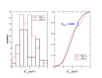
Figure 2: The X-ray $E_{p}$ distribution of UBLs (red) and TBLs (black). The sample of TBLs considered here does not include Mrk 421 and PKS 2155-304 and giant flares of Mrk 501 and 1H 1426+421, as described in Section 5. The maximum separation $D_{KS}$, of the two cumulative distributions, corresponding to the variable of the KS test, is also shown on the plot.

On the other hand, both the LP and the PEC models provide acceptable $\chi^{2}_{r}$ values for all the UBLs (Appendix and Figure 1, right panel), and neither model can be favored over the other in terms of $\chi^{2}_{r}$ and residuals. We performed a Kolmogorov-Smirnoff (KS) test of the two distributions of $\chi^{2}_{r}$ and found that they are similar at the 99% level of confidence.

However, it is noteworthy that the $E_{p}$ values derived using the PEC model have larger uncertainties than those derived with the LP model. This is because with the PEC model, $E_{p}$ is directly related to the exponential cut-off, which is determined by the high energy tail of the X-ray spectra, which is not well sampled.

On the other hand, the LP model provides a systematically better description than PEC function for the TBL X-ray spectra (M08). Thus to compare the TBL and UBL X-ray spectral properties, we adopted the LP model description.

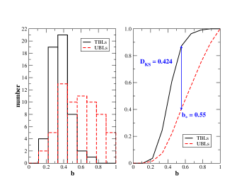
Figure 3: The X-ray curvature $b$ distribution of UBLs (red) and TBLs (black). The sample of TBLs considered here does not include Mrk 421, PKS 2155-304 and the giant flares of Mrk 501 and 1H 1426+421, as described in Section 5. The maximum separation, $D_{KS}$, of the two cumulative distributions (i.e., the variable used for the KS test) and the corresponding boundary value of the curvature $b_{*}$ are also shown on the plot.

We found the following trends among the spectral parameters:

2. Peak energy $E_{p}$. The $E_{p}$ distribution for the UBLs is consistent with that of TBLs, exhibiting a peak around a value $\sim$ 1.75 keV (Figure 2, left panel). There is a hint of a difference above the $E_{p}=$ 2.5 keV; a KS test (Figure 2, right panel) shows that the two distributions do not differ at a confidence level of 99%.

In addition, if we identify X-ray flares of HBLs as states where both $E_{p}$ and $L_{p}$ increase above their average values, then the scarcity of high $E_{p}$ (i.e., higher than $\sim$ 5 keV) values found in our analysis suggests that TBLs are more variable than UBLs, because in random observations UBLs always appear in their quiescent state.

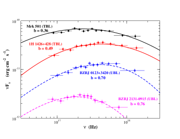
Figure 4: The unfolded X-ray SEDs for 4 HBLs: 2 UBLs (dashed lines), BZBJ 0123+3420 (blue open squares, 2009-08-28) and BZBJ 2131-0915 (magenta open squares, 2009-03-30), in comparison with 2 archival observations of the TBLs (solid lines): Mrk 501 (black filled circles, 2006-20-07) and 1H 1426+428 (red filled circles, 2006-03-07) (see M08 for more details). The TBL X-ray spectra are broader than the UBLs.

3. Spectral curvature $b$. There is a systematic difference in $b$ values between TBLs and UBLs (Figure 3, left panel). It is clear that the curvature in the latter is systematically higher, indicating that the UBL X-ray spectra spectra are narrower around $E_{p}$ than those of TBLs. Applying a KS test, the two distributions are different at a confidence level of 90%, and the maximum separation of the two cumulative distributions of $b$occurs at the boundary value $b_{*}$ = 0.55 (Figure 3, right panel). This implies that, given the two $b$ distributions , there is a low probability ($\sim$ 12%) of finding to find a TBL with X-ray spectral curvature higher than the boundary value $b_{*}$ (Figure 3, right panel). Thus $b_{*}$ permit us us to distinguish between TBLs and UBLs based on the X-ray spectral behavior. The stronger curvature in UBLs is also seen in the acceptable $\chi^{2}_{r}$ values when the PEC model is adopted. This occurs because the PEC model mimics high values of the spectral curvature due to its exponential cut-off than a typical LP model with $b\sim$ 0.5.

4. Spectral parameter trends. There is no clear correlation for the UBLs in the acceleration plane ($E_{p}$ vs $b$), while for TBLs $E_{p}$ and $b$ anti-correlate (M08). On the other hand, there is no significant trend between $L_{p}$ and $b$ in either the UBLs or the TBLs (M08). All correlation coefficients evaluated between spectral parameters are lower than 0.1 for both LP and PEC models.

5.2 Variability

The UBL X-ray fluxes derived from our archival Swift andXMM-Newton  analysis (from December 2004 to October 2010) are consistent within a factior of $\sim$2 with those measured, in the same energy range (i.e. 0.1-2.4 keV), $\sim$ 15 years earlier ROSAT observations (from June 1990 to February 1999), as listed in the ROMA BZCAT (Massaro et al. 2010b). The ROSAT fluxes and those derived from our spectral analysis are reported in Appendix. Only 18% of the selected UBLs show a flux ratio: $\rho=<F_{0.1-2.4keV}>/F_{ROSAT}$ higher than 2 (see Figure 5). This suggests that UBLs vary little on a 20 year timescale, unlike TBLs which can show variability by a factor of $\sim$ 5-10 over 1 year timescale.

Figure 5: The ratio $\rho$ between the ROSAT X-ray flux and the one derived from our analysis, for the selected UBLs. evaluated in the same energy range (i.e. $<$F_0.1-2.4keV$>$)

5.3 Fermi LAT Properties

The majority, 80%,of TBLs known up to October 2010 (19 out of 24) have been also detected in the “GeV” Fermi  LAT energy range (30 MeV - 100 GeV) (Abdo et al., 2010). We searched the Fermi catalog for detections of UBLs and we found that only $\sim$ 20% (24 out of 118) were detected. However, for the selected sample of 47 sources investigated here $\sim$ 40% (19 out of 47) were detected by the Fermi  LAT. Because the majority of TBLs have been detected by Fermi, this could appear to be a requirement for being a TeV source. However spectral variability may make them undetectable if they lie close to the Fermi detection threshold.

We compared the properties of TBLs and UBLs detected by Fermi to see if there are differences in their $\gamma$-ray properties. The Fermi LAT “GeV” luminosity $L_{\gamma}$ vs. redshift is shown in Figure 6a. There is a marginal indication that for the Fermi detections the UBLs are less luminous than TBLs, in particular at low redshifts, in agreement with the fact that a most ($\sim$ 50%) of them in our have not been detected.

The range of values of the $\gamma$-ray spectral index $a_{\gamma}$ is a similar between the TBLs and the UBLs detected by the Fermi LAT (Figure 6b), the variance of the two distributions are 0.06 and 0.07, respectively. Figure 6b shows the $\gamma$-ray photon index $a_{\gamma}$ vs. the average X-ray photon index $<a_{X}>$ from the LP model, weighted with the inverse of the variance.

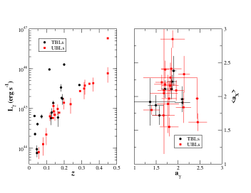
Figure 6: The $\gamma$-ray (30 MeV - 100 GeV) luminosity for UBLs (red squares) and TBLs (black circles) evaluated using the $\gamma$-ray fluxes reported in the first year Fermi catalog (Abdo et al., 2010). The Fermi LAT$\gamma$-ray photon index $\Gamma$ for UBLs (red square) and TBLs (black circles) with respect to the mean X-ray photon index $<a>$.

We conclude that the MeV-GeV $\gamma$-ray spectral behavior of the UBLs is similar to that of the TBLs, and the only differences appear to reside in the normalization of their $\gamma$-ray flux. However, this conclusions are valid for those UBLs bright enough in the LAT energy range to be detected by Fermi during one year. The non-detected HBL could have a different $\gamma$-ray spectral behavior that cannot be investigated with the present data set.

6 HBLs Detectable at TeV Energies

From comparing the distribution of the X-ray spectral curvature and the GeV Fermi LAT detections, we propose criteria to predict which UBLs are more likely to be detectable at TeV energies.

TeV energies lie beyond the inverse Compton peak of the HBL SEDs. Hence to be detectable they need both a high GeV flux level and a small GeV - TeV spectral curvature. In the SSC scenario, the X-ray spectral curvature, $b$, of HBLs, evaluated at the synchrotron SED peak, $E_{p}$, is a good predictor of the curvature of the inverse Compton peak at GeV - TeV energies, although they are not always identical (Massaro et al., 2006).

We can define three levels of confidence (i.e., TeV classes) in the prediction of TeV detectability (see Table 2, Col. 12):

Class 1: the best candidates for the future TeV detections are provided by UBLs with a GeV Fermi LAT detection and a curvature, $b$, lower than $b_{*}$ in all the X-ray observations (see Figure 3b). We found that four UBLs satisfy both conditions and so are the most likely new TeV detectable extragalactic sources: BZB J0326+0225, BZB J0442-0018, BZB J0744+7433 and BZB J1743+1953. Spectral variability could limit this prediction but UBLs appear to be less variable in the X-ray band than TBLs (see Section 6.2 and Figure 5).

Class 2: six more UBLs have some X-ray observations with $b<b_{*}$, and are also detected by Fermi LAT and so are still TeV candidates: BZB J0208+3523, BZB J1136+6737, BZB J1417+2543, BZB J1442+1200, BZB J1728+5013, BZB J2250+3824 The variability of $b$ leads us to expect the discovery of other new TBLs when their X-ray spectrum has $b$ $\leq$ $b_{*}$.

Class 3: UBLs with $b$ $\leq$ $b_{*}$ in at least one X-ray observations and $F_{X}$ $\geq$ 10^-11 erg s^-1 cm^-2 in the 0.5-10 keV energy range, but no LAT detection, make up our third class. The lower GeV normalization makes these less likely TeV candidates. However, in the single zone SSC scenario (e.g., Paggi et al., 2009), the X-ray flux is similar to the detection threshold of 1yr Fermi LAT $\gamma$-ray flux ((Atwood et al., 2009)) and the curvature is as broad as that of TBLs, we suggest that such UBLs can be detected at TeV energies. Five more UBLs fit class 3: BZB J0013-1854, BZB J0123+3420, BZB J0214+5144, BZB J1010-3119 and BZB J1253-3931.

Our source selection was concluded at the beginning of August 2010. Since then, of the 15 total candidates, the sources BZB J1442+1200 and BZB J2250+3824 from our class 2 and BZB J0013-1854 and BZB J1010-3119 from class 3 have been detected at TeV energies (see the TeV CAT for new announced TeV sources).

7 Summary

We have carried out an extensive X-ray spectral analysis of HBLs to compare the spectral behavior of those undetected at TeV energies (UBLs) with those already known as TeV emitters (TBLs). We analyzed all 135 X-ray observations of a sample of 47 UBLs present in the XMM-Newton and Swift archives up to August 2010.

We found that the $E_{p}$ distributions of UBLs and TBLs are similar, and symmetric around a value of a few keV for both subclasses. Instead the X-ray spectral curvature, $b$, of UBLs, is systematically lower than in TBLs, implying that the UBL X-ray spectra are narrower.

In addition, in the first year Fermi catalog (Abdo et al., 2010), we found that the UBL and TBL MeV-GeV $\gamma$-ray spectral behavior is similar, yet only $\sim$ 40% of our selected UBLs have been detected in the Fermi LAT energy range vs 80% of TBLs (Abdo et al., 2010).

On the basis of our analysis, we have developed criteria to predict likely TBLs. We present three lists with different levels of confidence for TeV detectability based on MeV-GeV flux level and keV spectral curvature, comprising a total of 15 TeV candidates. By December 2010, four of our candidates have already been detected at TeV energies, landing support to our selection criteria.

A crucial check for our TeV candidate criteria will be provided by X-ray monitoring of candidates from the different TeV classes, with simultaneous GeV and TeV observations, to investigate the variability timescales of the spectral curvature.

A theoretical interpretation of the $E_{p}$ and $b$ distributions, for both UBLs and TBLs, in terms of systematic and stochastic acceleration mechanisms will be presented in a forthcoming paper (Massaro et al., 2011b).

Appendix A Results of the X-ray spectral analysis for the UBLs

The following tables report the log of the selected X-ray observations and the values of the spectral parameters we have derived for UBLs in our sample.

In Swift Tables the column $Frame$ reports on the observation modality (PC for photon counting and WT for windowed timed, see also Section 3.2 for details), and $Exps$ means the exposure time in seconds.

In XMM-Newton Table, $Frame$ indicates the EPIC camera used (M1$=$MOS1 and M2$=$MOS2), the modes (PW$=$partial window and FW$=$full window) and the filter (Th$=$thin, Md$=$medium, Tk$=$thick) used for each pointing (see Section 2.2 for details), and the exposure is reported in seconds in the column $Exps$.

All other columns in each table refer to bestfit with the log-parabolic model. When the value estimated for a spectral parameter is consistent with zero in a $2\sigma$ interval, the values reported in each table refer to the power-law model bestfit (see Section 4). In these cases, the curvature parameter $b$, the SED peak energy $E_{p}$ and the corresponding SED peak height $S_{p}$ cannot be reliably evaluated, and are marked with a dashed line.

Values of $E_{p}$ are reported in keV, the normalization $K$ in units of 10^-4 photons cm^-2 s^-1 keV^-1 and $S_{p}$ in units of 10^-13 erg cm^-2 s^-1 with $F_{X}$ denoting the 0.5-10 keV flux measured in units of 10^-11 erg cm^-2 s^-1.

Table 3: Swift  spectral analysis results with the LP model of the UBLs.

Obs ID	$Date$	Frame	Exps	$a$	$b$	$E_{p}$	$K$	$S_{p}$	$F_{X}$	$\chi^{2}_{r}$
BZB J0013-1854
00031806002	10/09/10	pc	3782	1.83(0.06)	0.68(0.15)	1.34(0.11)	34(1)	52.2(2.1)	1.24	1.43(36)
00031806003	10/09/10	pc	4193	1.89(0.05)	0.46(0.13)	1.31(0.14)	30(1)	48.1(1.7)	1.16	1.23(41)
sum	-	pc	7975	1.86(0.04)	0.59(0.09)	1.31(0.07)	33(1)	53.8(1.8)	1.24	1.31(75)
00031806004	10/09/12	pc	3848	1.88(0.05)	0.64(0.15)	1.24(0.11)	32(1)	52.7(2.1)	1.18	1.05(33)
00031806005	10/09/18	pc	2744	1.88(0.06)	0.36(0.19)	1.44(0.29)	28(1)	45.0(2.1)	1.14	1.20(24)
sum	-	pc	6592	1.87(0.04)	0.59(0.09)	1.28(0.08)	30(1)	49.3(1.4)	1.13	0.67(59)
BZB J0123+3420
00035000001	05/06/09	pc	1587	1.62(0.10)	0.64(0.21)	1.99(0.31)	85(5)	155.0(9.1)	3.56	0.70(15)
00035000002	06/07/06	pc	5414	1.70(0.06)	0.46(0.12)	2.11(0.28)	65(2)	115.8(4.1)	2.80	1.02(43)
00035000003	06/07/10	pc	2444	1.74(0.11)	0.33(0.22)	2.46(0.89)	70(4)	126.5(7.2)	3.18	1.61(18)
sum	-	pc	9445	1.63(0.04)	0.57(0.09)	2.13(0.17)	66(2)	122.5(3.2)	2.88	0.98(77)
00030876001	07/01/18	pc	782	1.39(0.20)	1.28(0.38)	1.73(0.18)	99(7)	188.5(14.8)	3.63	0.82(7)
00035000005	07/09/07	pc	1018	1.69(0.19)	-	-	72(6)	-	3.30	0.70(6)
00035000006	07/09/11	pc	521	-	-	-	-	-	-
00035000007	07/09/12	pc	521	-	-	-	-	-	-
00035000008	07/09/13	pc	511	-	-	-	-	-	-
00035000004	07/09/14	pc	699	-	-	-	-	-	-
sum	-	pc	3271	1.69(0.06)	0.76(0.14)	1.59(0.11)	76(3)	130.2(4.7)	2.81	1.09(39)
00035000009	07/09/15	pc	1289	1.60(0.18)	0.88(0.51)	1.57(0.24)	80(6)	143.4(13.5)	3.00	0.44(7)
00035000010	07/09/27	pc	754	1.69(0.24)	0.93(0.65)	1.46(0.24)	166(14)	282.1(26.1)	5.71	1.08(5)
00035000011	07/10/27	pc	1479	1.94(0.14)	-	-	65(4)	-	3.00	1.11(9)
sum	-	pc	3521	1.74(0.07)	0.70(0.17)	1.52(0.13)	77(3)	129.9(5.5)	2.83	1.43(30)
00035000013	07/11/09	pc	2105	1.80(0.10)	0.53(0.22)	1.53(0.23)	90(5)	150.0(8.4)	3.45	0.96(17)
00035000014	07/11/16	pc	1380	1.67(0.15)	0.52(0.37)	2.07(0.70)	84(6)	152.3(10.6)	3.62	1.80(10)
sum	-	pc	3485	1.78(0.06)	0.52(0.13)	1.62(0.16)	89(3)	149.8(5.4)	3.48	0.95(40)
00037298001	08/03/06	pc	1248	1.72(0.11)	0.33(0.24)	2.69(1.34)	73(4)	134.2(8.2)	3.05	0.83(17)
00037298002	08/06/08	pc	4757	1.69(0.06)	0.55(0.13)	1.92(0.20)	69(2)	122.6(4.4)	2.88	1.56(43)
00037298003	09/08/28	pc	4816	1.68(0.06)	0.70(0.13)	1.70(0.13)	74(2)	129.6(4.4)	2.88	0.57(45)
sum	-	pc		1.69(0.04)	0.63(0.07)	1.78(0.09)	75(2)	131.4(3.0)	2.99	0.99(96)
BZB J0201+0034
00038117001	09/06/05	pc	5041	1.94(0.08)	0.69(0.28)	1.10(0.14)	12(1)	18.8(1.1)	0.40	1.34(16)
BZB J0214+5144
00038333001	08/12/10	pc	5040	1.72(0.07)	0.65(0.13)	1.62(0.12)	49(1)	83.6(2.6)	1.67	0.96(53)
00038333002	08/12/11	pc	780	-	-	-	-	-	-
00038333003	09/09/16	pc	3376	1.65(0.09)	0.43(0.15)	2.58(0.45)	47(2)	89.2(3.4)	1.99	0.99(40)
sum	-	pc	9196	1.66(0.05)	0.61(0.09)	1.90(0.11)	47(1)	83.3(1.9)	1.73	1.10(95)
BZB J0227+0202
00037512001	08/06/24	pc	1308	-	-	-	-	-	-
00037512002	10/08/19	pc	2847	1.65(0.09)	0.70(0.23)	1.79(0.26)	26(1)	46.9(2.6)	1.09	0.66(17)
sum	-	pc	4156	1.73(0.08)	0.49(0.23)	1.89(0.45)	16(1)	27.1(1.4)	0.67	0.66(19)
BZB J0325-1646
00035005001	05/06/29	pc	7671	2.85(0.13)	-	-	3.9(0.3)	-	0.11	1.26(8)
00035005002	06/07/19	pc	1951	-	-	-	-	-	-
00035005003	07/06/08	pc	346	-	-	-	-	-	-
sum	-	pc	9969	2.92(0.11)	-	-	3.7(0.2)	-	0.10	1.07(11)
BZB J0326+0225
00035006001	05/06/26	pc	10680	2.28(0.08)	0.42(0.28)	0.52(0.21)	7.5(0.4)	13.5(1.5)	0.21	0.64(19)
00035006002	05/06/29	pc	4650	2.40(0.20)	-	-	7(1)	-	0.18	0.42(5)
00035006003	05/07/11	pc	6549	2.31(0.16)	-	-	4.7(0.4)	-	0.16	1.04(5)
sum	-	pc	21880	2.26(0.06)	0.43(0.14)	0.49(0.16)	6.4(0.2)	11.3(0.7)	0.18	0.86(35)
BZB J0441+1504
00036806002	08/01/08	pc	7059	1.18(0.15)	1.17(0.26)	2.23(0.17)	18(1)	40.4(1.7)	0.76	1.26(31)
BZB J0442-0018
00036312001	07/03/28	pc	1275	-	-	-	-	-	-
00036312003	07/04/17	pc	5259	-	-	-	-	-	-
00036312003	07/07/30	pc	2776	-	-	-	-	-	-
00036312005	08/10/19	pc	10780	1.97(0.30)	-	-	2.1(0.2)	-	0.09	0.28(3)
sum	-	pc	20090	1.87(0.13)	0.45(0.32)	1.39(0.33)	2.3(0.1)	3.8(0.3)	0.09	0.84(10)

Col. (7) $E_{p}$ is in keV.
Col. (8) $K$ is in 10^-4 photons cm^-2 s^-1 keV^-1.
Col. (9) $S_{p}$ is in units of 10^-13 erg cm^-2 s^-1.
Col. (10) $F_{X}$ denoting the 0.5-10 keV flux measured in units of 10^-11 erg cm^-2 s^-1.

Table 4: Swift  spectral analysis results with the LP model of the UBLs.

Obs ID	$Date$	Frame	Exps	$a$	$b$	$E_{p}$	$K$	$S_{p}$	$F_{X}$	$\chi^{2}_{r}$
BZB J0621-3411
00038819001	09/07/29	pc	949	0.90(0.52)	1.47(1.14)	2.37(0.78)	17(2)	43.4(5.1)	0.84	0.63(2)
BZB J0751+1730
00036808001	07/05/30	pc	3102	1.20(0.41)	1.33(0.88)	2.01(0.43)	6(1)	13.6(1.5)	0.27	0.09(4)
BZB J0753+2921
00036809001	08/03/06	pc	4500	-	-	-	-	-	-
BZB J0847+1133
00037396001	08/02/29	pc	2022	1.80(0.07)	-	-	33(2)	-	1.63	0.85(20)
BZB J0916+5238
00038165001	09/03/07	pc	7710	2.08(0.06)	0.55(0.18)	0.84(0.14)	9.5(0.4)	15.4(0.7)	0.32	0.65(23)
BZB J0930+4950
00039154001	10/10/12	pc	2869	1.67(0.06)	0.89(0.15)	1.53(0.11)	32(1)	54.8(2.3)	1.20	0.73(29)
BZB J0952+7502
00036810001	07/05/20	pc	9759	1.80(0.07)	0.44(0.16)	1.71(0.30)	7.3(0.3)	12.3(0.6)	0.31	0.89(23)
00036810002	07/10/04	pc	2230	-	-	-	-	-	-
sum	-	pc	11990	1.79(0.07)	0.58(0.17)	1.51(0.17)	7.1(0.3)	11.9(0.6)	0.28	1.30(26)
BZB J1010-3119
00030940002	07/05/17	pc	1481	2.00(0.09)	0.46(0.23)	1.00(0.24)	43(2)	68.9(3.4)	1.41	0.85(18)
00030940004	07/05/18	pc	1968	1.82(0.10)	1.13(0.25)	1.21(0.09)	42(2)	68.9(3.4)	1.18	1.08(20)
sum	-	pc	3700	1.88(0.06)	0.76(0.14)	1.21(0.09)	42(1)	67.4(2.4)	1.29	1.40(39)
BZB J1022+5124
00036811001	08/01/13	pc	5703	1.60(0.12)	-	-	8.6(0.5)	-	0.49	1.61(14)
BZB J1053+4929
00031594001	10/01/21	pc	5243	2.21(0.11)	1.01(0.46)	0.79(0.12)	6.4(0.5)	10.5(0.8)	0.18	1.67(8)
BZB J1056+0252
00037547001	07/06/08	pc	4725	1.65(0.07)	0.59(0.15)	1.97(0.25)	20(1)	35.6(1.5)	0.84	1.02(29)
BZB J1111+3452
00038219001	09/04/18	pc	4590	-	-	-	-	-	-
BZB J1117+2014
00038451001	09/04/20	pc	1341	2.40(0.13)	0.69(0.59)	0.52(0.32)	22(2)	39.3(4.8)	0.61	0.72(6)
BZB J1136+6737
00037135001	07/05/25	pc	2788	1.60(0.09)	0.96(0.23)	1.60(0.14)	49(3)	85.8(4.8)	1.87	0.98(17)
00037135002	07/05/30	pc	4487	1.74(0.07)	0.68(0.19)	1.54(0.16)	44(2)	74.3(3.6)	1.74	0.71(22)
00037135003	08/02/16	pc	4291	1.49(0.05)	0.68(0.10)	2.37(0.23)	95(3)	189.2(5.7)	4.56	0.85(62)
00036812001	08/01/29	pc	3983	1.47(0.07)	0.42(0.14)	4.26(1.57)	49(2)	115.4(8.3)	2.83	1.00(28)
00036812002	08/01/30	pc	2304	1.66(0.09)	0.38(0.19)	2.40(0.72)	51(3)	89.1(4.8)	2.56	1.06(16)
BZB J1145-0340
00036813001	07/11/09	pc	2870	-	-	-	-	-	-
00036813002	07/12/06	pc	2934	1.64(0.17)	1.26(0.43)	1.39(0.15)	9(1)	14.6(1.3)	0.28	0.57(5)
sum	-	pc	5805	1.87(0.11)	1.02(0.37)	1.16(0.13)	8(1)	12.5(0.9)	0.25	1.21(10)
BZB J1154-0010
00038231001	09/11/08	pc	1209	-	-	-	-	-	-
BZB J1237+6258
00042002001	06/11/12	pc	3114	-	-	-	-	-	-
00042002008	06/02/15	pc	6501	2.10(0.06)	0.44(0.22)	0.77(0.16)	12(1)	20.0(0.8)	0.43	1.02(25)
00060001001	06/11/14	pc	2677	-	-	-	-	-	-
sum	-	pc	12290	2.17(0.05)	0.47(0.18)	0.6590.14)	7.5(0.3)	12.5(0.48)	0.25	0.99(30)
00066002001	07/04/18	pc	748	-	-	-	-	-	-
00042002024	07/03/22	pc	3664	2.10(0.12)	-	-	6(1)	-	2.28	0.70(5)
00042002018	07/06/12	pc	1593	1.80(0.18)	1.02(0.75)	1.25(0.26)	12(1)	19.4(2.1)	0.40	0.33(3)
00042002028	07/10/10	pc	1124	-	-	-	-	-	-	-
sum	-	pc	7129	1.93(0.08)	0.59(0.20)	1.15(0.15)	8.2(0.4)	13.2(0.7)	0.30	0.48(18)
00042002027	08/03/03	pc	1845	-	-	-	-	-	-
00038250001	09/03/10	pc	2769	-	-	-	-	-	-
00038250002	09/04/23	pc	3062	2.54(0.34)	-	-	2.7(0.6)	-	0.09	0.65(3)
00042002034	09/10/25	pc	910	-	-	-	-	-	-
sum	-	pc	8587	2.26(0.11)	0.82(0.44)	0.70(0.16)	3.9(0.3)	6.6(0.5)	0.11	1.18(9)
00042002035	10/01/27	pc	4729	2.07(0.14)	-	-	5.1(0.4)	-	0.19	0.79(5)
00042002038	10/10/13	pc	1568	-	-	-	-	-	-
sum	-	pc	8587	1.98(0.13)	0.68(0.42)	1.03(0.22)	4.2(0.4)	6.8(0.6)	0.15	0.58(7)

Col. (7) $E_{p}$ is in keV.
Col. (8) $K$ is in 10^-4 photons cm^-2 s^-1 keV^-1.
Col. (9) $S_{p}$ is in units of 10^-13 erg cm^-2 s^-1.
Col. (10) $F_{X}$ denoting the 0.5-10 keV flux measured in units of 10^-11 erg cm^-2 s^-1.

Table 5: Swift  spectral analysis results with the LP model of the UBLs.

Obs ID	$Date$	Frame	Exps	$a$	$b$	$E_{p}$	$K$	$S_{p}$	$F_{X}$	$\chi^{2}_{r}$
BZB J1253-3931
00037538001	08/12/20	pc	4651	1.46(0.11)	0.41(0.21)	4.68(2.68)	20(1)	47.5(4.7)	1.08	0.65(25)
BZB J1257+2412
00031203001	08/05/09	pc	2200	1.89(0.10)	0.55(0.28)	1.25(0.22)	17(1)	28.3(1.9)	0.66	0.98(11)
BZB J1341+3959
00038268001	08/10/15	pc	5198	1.63(0.06)	0.70(0.14)	1.84(0.18)	23(1)	41.2(1.5)	0.98	0.96(37)
00038268002	09/12/21	pc	5901	1.64(0.07)	0.70(0.16)	1.82(0.19)	14.0(0.6)	25.1(1.2)	0.60	1.42(26)
sum	-	pc	11100	1.66(0.04)	0.66(0.10)	1.82(0.14)	18.1(0.5)	32.3(0.1)	0.78	1.04(63)
00040599001	10/10/10	pc	854	-	-	-	-	-	-	-
00040599002	10/10/15	pc	3947	1.55(0.09)	0.66(0.21)	2.20(0.38)	13(1)	25.7(1.5)	0.63	1.03(17)
sum	-	pc	4801	1.60(0.08)	0.50(0.20)	2.53(0.75)	13(1)	25.0(1.4)	0.64	1.42(21)
BZB J1417+2543
00035270001	05/12/20	pc	8547	1.83(0.04)	0.43(0.08)	1.59(0.14)	64(2)	106.6(2.9)	2.69	0.92(69)
00056620002	05/05/26	pc	775	1.72(0.15)	0.88(0.59)	1.44(0.34)	84(7)	142.1(11.6)	3.08	0.57(6)
00056620002	26/05/05	wt	1015	1.87(0.07)	0.51(0.19)	1.34(0.18)	81(4)	132.8(6.2)	1.52	0.75(25)
00035270002	06/07/11	pc	1882	1.90(0.09)	-	-	60(4)	-	2.93	0.58(13)
00031204001	08/05/10	pc	1694	1.75(0.10)	0.39(0.34)	2.08(1.24)	51(2)	86.8(6.7)	2.25	1.78(10)
00031204002	08/05/30	pc	1664	2.03(0.11)	0.63(0.38)	0.94(0.21)	49(4)	78.3(5.6)	1.64	0.39(8)
sum	-	pc	3358	1.87(0.07)	0.53(0.19)		49(2)		1.91	1.36(23)
BZB J1439+3932
00037514002	08/10/15	pc	1458	2.49(0.16)	-	-	17(2)	-	0.56	0.38(5)
00037514001	08/06/07	pc	832	2.18(0.27)	-	-	19(3)	-	0.78	1.86(2)
sum	-	pc	2290	2.42(0.08)	0.64(0.29)	0.47(0.17)	18(1)	33.6(2.6)	0.52	0.82(12)
BZB J1442+1200
00031218002	08/06/12	pc	1732	1.83(0.11)	0.37(0.34)	1.70(0.68)	40(2)	66.9(4.8)	1.73	1.27(9)
00031218003	10/02/26	pc	1110	2.15(0.18)	-	-	42(5)	-	1.59	0.12(3)
00031218005	10/03/09	pc	1058	1.80(0.20)	1.36(0.57)	1.18(0.15)	43(4)	70.2(6.4)	1.27	1.79(3)
00040617002	10/12/09	pc	3308	1.82(0.32)	0.32(0.16)	1.93(0.52)	56(2)	94.7(4.3)	2.50	0.94(27)
sum	-	pc	7208	1.85(0.05)	0.48(0.11)	1.43(0.13)	51(2)	83.3(2.7)	2.03	0.90(49)
BZB J1534+3715
00038300001	08/12/12	pc	14760	2.87(0.15)	-	-	1.3(0.1)	-	0.04	0.85(4)
BZB J1605+5421
00038303001	09/01/18	pc	7066	1.37(0.12)	0.84(0.33)	2.36(0.61)	5.0(0.3)	10.5(0.8)	0.24	0.94(10)
BZB J1728+5013
00040635002	10/04/02	pc	260	-	-	-	-	-	-	-
00040635001	10/04/05	pc	1395	1.98(0.10)	0.60(0.34)	1.03(0.19)	52(3)	82.7(5.7)	1.78	0.57(10)
00040635003	10/04/05	pc	2150	2.12(0.08)	-	-	45(3)	-	1.66	0.93(14)
00040635004	10/05/01	pc	1667	2.12(0.08)	0.64(0.26)	0.81(0.14)	38(2)	62.1(3.3)	1.21	1.02(16)
sum	-	pc	5473	2.12(0.05)	0.46(0.15)	0.74(0.15)	47(2)	76.0(2.8)	1.57	0.80(31)
BZB J1743+1935
00030950001	07/06/15	pc	1918	1.97(0.09)	0.35(0.24)	1.11(0.30)	37(2)	59.8(3.1)	1.34	1.90(19)
00040639001	10/07/10	pc	860	2.01(0.24)	-	-	36(3)	-	1.41	0.63(5)
sum	-	pc	2779	1.92(0.07)	0.47(0.19)	1.22(0.18)	37(2)	60.0(2.5)	1.30	1.25(27)
BZB J2131-0915
00037543001	09/03/30	pc	5189	2.16(0.06)	0.76(0.22)	0.78(0.10)	16(1)	26.6(1.2)	4.69	0.96(23)
BZB J2201-1707
00036814001	07/12/08	pc	4538	1.52(0.17)	0.92(0.42)	1.82(0.32)	7(1)	12.8(1.0)	0.28	0.65(7)
00036814002	07/12/11	pc	5991	2.09(0.12)	-	-	7(1)	-	0.26	0.64(10)
sum	-	pc	10530	1.89(0.08)	0.40(0.18)	1.36(0.23)	7.0(0.3)	11.4(0.6)	0.28	0.67(21)

Col. (7) $E_{p}$ is in keV.
Col. (8) $K$ is in 10^-4 photons cm^-2 s^-1 keV^-1.
Col. (9) $S_{p}$ is in units of 10^-13 erg cm^-2 s^-1.
Col. (10) $F_{X}$ denoting the 0.5-10 keV flux measured in units of 10^-11 erg cm^-2 s^-1.

Table 6: Swift  spectral analysis results with the LP model of the UBLs.

Obs ID	$Date$	Frame	Exps	$a$	$b$	$E_{p}$	$K$	$S_{p}$	$F_{X}$	$\chi^{2}_{r}$
BZB J2250+3824
00039211001	09/08/10	pc	1110	2.34(0.31)	-	-	27(2)	-	0.84	1.18(4)
00039211002	10/02/18	pc	2996	2.47(0.14)	-	-	15(1)	-	0.42	1.27(8)
00040151001	10/04/17	pc	1654	2.97(0.82)	-	-	15(2)	-	0.34	1.25(3)
00039211003	10/04/18	pc	3446	2.55(0.12)	-	-	17(1)	-	0.38	1.11(11)
sum	-	pc	9205	2.43(0.06)	0.29(0.18)	0.19(0.02)	17(1)	39.4(12.3)	0.45	0.66(33)
00039211005	10/10/05	pc	1741	2.01(0.11)	1.19(0.26)	0.99(0.11)	52(2)	84.1(3.9)	1.24	0.72(18)
00039211006	10/10/06	pc	4130	2.19(0.08)	0.98(0.25)	0.80(0.10)	70(3)	114.1(5.1)	1.62	0.55(23)
00039211007	10/10/07	pc	3135	2.38(0.07)	-	-	58(2)	-	1.75	1.09(17)
00039211008	10/10/08	pc	782	-	-	-	-	-	-	-
00039211009	10/10/09	pc	143	-	-	-	-	-	-	-
sum	-	pc	9932	2.17(0.03)	0.81(0.08)	0.78(0.05)	62(1)	100.8(1.9)	1.52	1.16(111)
00039211010	10/10/10	pc	1429	2.07(0.13)	0.87(0.46)	0.91(0.20)	49(3)	78.0(4.8)	1.24	1.20(12)
00039211011	10/10/11	pc	3655	2.05(0.07)	0.52(0.19)	0.90(0.17)	49(2)	79.1(2.9)	1.47	1.02(33)
sum	-	pc	5084	2.07(0.06)	0.63(0.14)	0.88(0.11)	49(1)	79.5(2.4)	1.38	1.06(47)
00039211012	10/10/12	pc	4933	2.04(0.09)	0.66(0.21)	0.93(0.16)	62(3)	100.2(4.2)	1.76	1.22(25)
00039211013	10/10/13	pc	4382	1.80(0.09)	0.79(0.20)	1.33(0.12)	69(3)	114.4(4.9)	2.18	0.68(26)
sum	-	pc	9316	1.91(0.06)	0.78(0.13)	1.14(0.08)	64(2)	103.3(3.0)	1.87	0.96(55)
00039211014	10/10/14	pc	4676	1.91(0.09)	0.87(0.25)	1.12(0.11)	63(3)	100.7(4.3)	1.76	1.26(27)
00039211015	10/10/15	pc	5316	2.02(0.05)	1.01(0.14)	0.97(0.06)	52(1)	82.8(2.4)	1.29	1.11(53)
00039211016	10/10/16	pc	3304	2.02(0.07)	0.84(0.19)	0.97(0.10)	56(2)	89.2(3.4)	1.48	0.95(31)
sum	-	pc	13300	1.91(0.05)	1.22(0.13)	1.09(0.05)	57(1)	91.6(2.4)	1.41	0.93(64)
BZB J2308-2219
00036815001	07/09/29	pc	7289	1.95(0.20)	-	-	3(1)	-	0.13	0.74(3)
BZB J2322+3436
00040684001	10/02/17	pc	1344	-	-	-	-	-	-	-
00040684002	10/02/17	pc	3523	2.28(0.22)	-	-	4(1)	-	0.14	1.70(2)
sum	-	pc	4866	2.16(0.30)	-	-	5(1)	-	0.14	1.26(3)
BZB J2343+3439
00037545001	08/05/30	pc	2381	1.60(0.13)	1.34(0.30)	1.40(0.10)	24(1)	41.7(2.5)	0.73	1.17(14)
00037545002	08/06/02	pc	3336	1.78(0.09)	0.82(0.22)	1.35(0.13)	24(1)	39.3(1.9)	0.79	0.90(20)
sum	-	pc	5717	1.69(0.07)	0.99(0.17)	1.43(0.08)	24(1)	39.8(1.5)	0.77	1.14(36)

Col. (7) $E_{p}$ is in keV.
Col. (8) $K$ is in 10^-4 photons cm^-2 s^-1 keV^-1.
Col. (9) $S_{p}$ is in units of 10^-13 erg cm^-2 s^-1.
Col. (10)$F_{X}$ denoting the 0.5-10 keV flux measured in units of 10^-11 erg cm^-2 s^-1.

Table 7: XMM-Newton  spectral analysis results with the LP model of the UBLs.

Obs ID	$Date$	Frame	Exps	$a$	$b$	$E_{p}$	$K$	$S_{p}$	$F_{X}$	$\chi^{2}_{r}$
BZB J0208+3523
0084140101	01/02/14	M1-FW(Me)	38070	2.09(0.03)	0.61(0.07)	0.85(0.06)	8.1(0.1)	13.0(0.2)	0.24	0.92(134)
0084140501	02/02/04	M1-FW(Me)	11680	1.95(0.05)	0.41(0.11)	1.16(0.14)	8.7(0.2)	13.9(0.3)	0.31	1.13(69)
BZB J0326+0225
0094382501	02/02/05	M1-PW(Me)	4563	2.36(0.07)	0.32(0.16)	0.27(0.21)	18.4(0.4)	36.6(7.3)	0.50	0.68(47)
BZB J0441+1504
0203160101	03/09/05	M1-PW(Th)	7438	2.18(0.17)	-	-	3.3(0.1)	-	0.11	1.57(15)
BZB J0744+7433
0123100101	00/04/13	M1-PW(Th)	10620	2.17(0.03)	0.16(0.06)	0.28(0.18)	25.6(0.3)	45.8(3.6)	0.94	1.01(135)
0123100201	00/04/12	M1-PW(Th)	19580	2.19(0.03)	0.18(0.06)	0.30(0.15)	23.4(0.3)	42.0(2.8)	0.84	1.00(141)
BZB J1231+6414
0124900101	00/05/21	M1-FW(Th)	16220	2.15(0.04)	0.25(0.08)	0.50(0.18)	9.4(0.1)	15.9(0.7)	0.34	1.05(105)
BZB J1237+6258
0604830201	09/07/09	M2-FF(Th)	9847	1.83(0.09)	0.60(0.19)	1.40(0.14)	5.4(0.2)	9.0(0.3)	0.21	0.85(41)
BZB J1257+2412
0094383201	02/12/12	M2-SW(Md)	5788	2.00(0.04)	-	-	20.9(0.4)	-	0.98	1.06(95)
BZB J1510+333
0303930101	06/01/02	M2-FF(Th)	9844	1.64(0.02)	0.45(0.11)	2.53(0.35)	7.8(0.2)	14.9(0.4)	0.38	1.14(64)
BZB J1626+3513
0505010501	07/08/17	M2-FF(Md)	7696	2.50(0.15)	-	-	3.4(0.1)	-	0.10	0.65(12)
0505011201	07/08/19	M2-FF(Md)	15300	2.50(0.09)	-	-	3.5(0.1)	-	0.11	0.93(28)

Col. (7) $E_{p}$ is in keV.
Col. (8) $K$ is in 10^-4 photons cm^-2 s^-1 keV^-1.
Col. (9) $S_{p}$ is in units of 10^-13 erg cm^-2 s^-1.
Col. (10)$F_{X}$ denoting the 0.5-10 keV flux measured in units of 10^-11 erg cm^-2 s^-1.

Table 8: UBLs selected.

BZCAT Name	$F_{ROSAT}$	$<F_{0.1-2.4keV}>$	$\rho$
BZB J0013-1854	6.488	8.7675	0.74
BZB J0123+3420	25.254	19.6538	1.28
BZB J0201+0034	3.526	3.26	1.08
BZB J0208+3523	2.879	1.935	1.49
BZB J0214+5144	4.579	8.449	0.54
BZB J0227+0202	18.184	7.03	2.59
BZB J0325-1646	27.164	1.48	18.35
BZB J0326+0225	12.038	1.36	8.85
BZB J0441+1504	10.195	3.62	2.82
BZB J0442-0018	1.673	0.55	3.04
BZB J0621-3411	1.838	4.34	0.43
BZB J0744+7433	6.291	4.09	0.65
BZB J0751+1730	1.781	1.53	1.16
BZB J0753+2921	1.287	-	-
BZB J0847+1133	11.006	9.39	1.17
BZB J0916+5238	3.833	2.98	1.29
BZB J0930+4950	16.672	8.85	1.88
BZB J0952+7502	2.485	2.09	1.18
BZB J1010-3119	10.149	8.794	1.15
BZB J1022+5124	3.442	2.75	1.25
BZB J1053+4929	0.821	1.86	0.44
BZB J1056+0252	6.903	5.07	1.36
BZB J1111+3452	3.998	-	-
BZB J1117+2014	33.576	7.22	4.65
BZB J1136+6737	14.752	17.02	0.87
BZB J1145-0340	4.101	2.16	1.90
BZB J1154-0010	2.475	-	-
BZB J1231+6414	2.489	2.07	1.20
BZB J1237+6258	2.284	2.549	0.90
BZB J1253-3931	7.046	4.59	1.54
BZB J1257+2412	7.221	5.35	1.35
BZB J1341+3959	5.152	5.03	1.02
BZB J1417+2543	15.304	18.40	0.83
BZB J1439+3932	11.076	7.325	0.66
BZB J1442+1200	7.82	7.324	1.07
BZB J1510+3335	2.525	2.32	1.09
BZB J1534+3715	0.228	0.69	0.33
BZB J1605+5421	3.874	1.45	2.67
BZB J1626+3513	0.837	1.42	0.59
BZB J1728+5013	20.374	13.1	1.55
BZB J1743+1935	4.231	8.36	0.51
BZB J2131-0915	7.302	4.20	1.74
BZB J2201-1707	2.368	1.875	1.26
BZB J2250+3824	2.449	9.05	0.27
BZB J2308-2219	4.27	0.89	4.80
BZB J2322+3436	1.091	1.03	1.06
BZB J2343+3439	5.43	5.195	1.04

$F_{ROSAT}$ is in units of $10^{-12}erg~{}cm^{-2}~{}s^{-1}$.
$<F_{0.1-2.4keV}>$ is in units of $10^{-12}erg~{}cm^{-2}~{}s^{-1}$.

References

- Abdo et al. (2010) Abdo A. A. et al. 2010, ApJ, 710, 1271
- Abdo et al. (2011) Abdo A. A. et al. 2011 ApJ submitted arXiv: 1106.1348
- Aleksic et al. (2011) Aleksic, J. et al. 2011 A&A submitted arXiv: 1106.1589
- Acciari et al. (2011) Acciari, V. A. et al. 2011 A&A submitted arXiv: 1106.1210
- Atwood et al. (2009) Atwood, W. B. et al. 2009, ApJ, 697, 1071
- Aharonian et al. (2009) Aharonian, F. et al. 2009, A&A, 502, 749
- Albert et al. (2008) Albert, J. et al. 2008 Sci, 320, 1752
- Arnaud (1996) Arnaud, K.A., 1996, ”Astronomical Data Analysis Software and Systems V”, eds. Jacoby G. and Barnes J., p17, ASP Conf. Series volume 101
- Blandford & Rees (1978) Blandford, R. D., Rees, M. J., 1978, PROC. P̈ittsburgh Conference on BL Lac objects”, 328
- Blandford & Znajek (1977) Blandford, R. D., Znajek, R. L. 1977 MNRAS, 179, 433
- Blustin et al. (2004) Blustin, A. J., Page, M. J., Branduardi-Raymont, G., 2004, A&A, 417, 61
- Burrows et al. (2005) Burrows, D., Hill, J. E., Nousek, J. A., et al. 2005, SSRv., 120, 165
- Campana et al. (2009) Campana, R., Massaro, E., Mineo, T., 2009, A&A, 499, 847
- Cavaliere & D’Elia (2002) Cavaliere, C. & D’Elia V. 2002 ApJ, 571, 226
- Dwek & Krennrich (2005) Dwek, E. & Krennrich, F. 2005 ApJ, 618, 657
- Dunkley (2009) Dunkley, J., 2009 ApJ, 701, 1804
- Elvis et al. (1992) Elvis, M., Plummer, D., Schachter, J., Fabbiano, G. 1992 ApJS, 80, 257
- Freeman et al. (2001) Freeman, P., Doe, S., & Siemiginowska, A. 2001, Proc. SPIE, 4477, 76
- Giommi et al. (2005) Giommi, P.; Piranomonte, S.; Perri, M.; Padovani, P., 2005, A&A, 434, 385
- Hill et al. (2004) Hill, J.E., Burrows, D.N., Nousek, J.A. et al., 2004, SPIE, 5165, 217
- Grigis & Benz (2008) Grigis, P. G. & Benz A. O. 2008 ApJ, 683, 1180
- Inoue & Takahara (1996) Inoue, S., Takahara F., 1996, ApJ, 463, 555
- Kalberla et al. (2005) Kalberla, P.M.W., Burton, W.B., Hartmann, D., 2005, A&A, 440, 775
- Kardashev (1962) Kardashev, N. S., 1962, SvA, 6, 317
- Jones et al. (1974) Jones, T. W., O’Dell, S. L., & Stein, W. A. 1974, ApJ, 188, 353
- Landau et al. (1986) Landau, R., Golish, B., Jones, T. J., et al. 1986, ApJ, 308, L78
- Laurent-Muehleisen et al. (1999) Laurent-Muehleisen S. A. et al. 1999 ApJ, 525, 127
- Litvinenko (1996) Litvinenko, Y. E. 1996 ApJ, 462, 997
- Litvinenko (1999) Litvinenko, Y. E. 1999 A&A, 349, 685
- Lockman & Savage (1995) Lockman, F. J., & Savage, B. D., 1995, ApJS, 97, 1
- Loiseau et al. (2004) Loiseau, N., et al., 2004, ”User’s guide to the XMM-Newton Science Analysis System” (issue 3.1)
- Marscher & Gear (1985) Marscher, A. P., Gear, W. K. 1985, ApJ, 298, 114
- Maselli & Massaro (2009) Maselli, A. & Massaro, E. 2009, AN, 330, 295
- Massaro et al. (2004) Massaro, E., Perri, M., Giommi, P., et al. 2004, A&A, 422, 103
- Massaro et al. (2006) Massaro, E., Tramacere, A., Perri, M., Giommi, P., Tosti, G., 2006, A&A, 448, 861
- M08 (2008) Massaro, F., Tramacere A., Cavaliere A., et al. A&A 2008a, 478, 395 (M08)
- Massaro et al. (2008b) Massaro, F., Giommi, P., Tosti, G., A&A 2008b, 489, 1047
- Massaro et al. (2009) Massaro, E. et al. 2009 A&A, 495, 691
- Massaro et al. (2010a) Massaro, F., Grindlay, J. E., Paggi, A. 2010a, ApJL, 714, 299
- Massaro et al. (2010b) Massaro, E. et al. 2010b A&A submitted http://arxiv.org/abs/1006.0922
- Massaro et al. (2011a) Massaro, F., & Grindlay, J. E. 2011b ApJ, 727L, 1
- Massaro et al. (2011b) Massaro, F., A. Paggi, & A. Cavaliere, 2011a ApJL submitted
- Moretti et al. (2005) Moretti et al. 2005 SPIE, 5898, 360
- Padovani & Giommi (1995) Padovani, P., & Giommi, P., 1995, MNRAS, 277, 1477
- Paggi et al. (2009) Paggi, A., Massaro, F., Vittorini, V. et al. 2009 A&A, 504, 821
- Perri et al. (2007) Perri, M., Maselli, A., Giommi, P., et al., 2007, A&A, 462,889
- Perlman et al. (1996) Perlman, E. S. et al. 1996 ApJS, 104, 251
- Scarpa et al. (1999) Scarpa, R. et al. 1999 ApJ, 521, 134
- Snowden et al. (2004) Snowden, S., et al., 2004, ”The XMM-Newton ABC Guide” (version 2.01)
- Stawarz & Petrosian (2008) Stawarz & Petrosian 2008, ApJ, 681, 1725
- Struder et al. (2001) Struder, L., et al., 2001, A&A, 365, L18
- Tanihata et al. (2004) Tanihata, C., Kataoka, J., Takahashi, T., et al. 2004, ApJ, 601, 759,
- Tramacere et al. (2007) Tramacere, A., Massaro, F., Cavaliere, A., 2007, A&A, 466, 521
- Tramacere et al. (2009) Tramacere, A., Giommi, P., Perri, M. et al. 2009 A&A, 501, 879
- Turner et al. (2001) Turner, M. L. J., et al. 2001, A&A, 365, L27
- Urry et al. (2000) Urry, C. M. et al. 2000 ApJ, 532, 816