Performance Analysis of $l_{0}$ Norm Constraint Least Mean Square Algorithm

Abstract

As one of the recently proposed algorithms for sparse system identification, $l_{0}$ norm constraint Least Mean Square ($l_{0}$-LMS) algorithm modifies the cost function of the traditional method with a penalty of tap-weight sparsity. The performance of $l_{0}$-LMS is quite attractive compared with its various precursors. However, there has been no detailed study of its performance. This paper presents comprehensive theoretical performance analysis of $l_{0}$-LMS for white Gaussian input data based on some assumptions which are reasonable in a large range of parameter setting. Expressions for steady-state mean square deviation (MSD) are derived and discussed with respect to algorithm parameters and system sparsity. The parameter selection rule is established for achieving the best performance. Approximated with Taylor series, the instantaneous behavior is also derived. In addition, the relationship between $l_{0}$-LMS and some previous arts and the sufficient conditions for $l_{0}$-LMS to accelerate convergence are set up. Finally, all of the theoretical results are compared with simulations and are shown to agree well in a wide range of parameters.

Keywords: adaptive filter, sparse system identification, $l_{0}$-LMS, mean square deviation, convergence rate, steady-state misalignment, independence assumption, white Gaussian signal, performance analysis.

1 Introduction

Adaptive filtering has attracted much research interest in both theoretical and applied issues for a long time[1, 2, 3]. Due to its good performance, easy implementation, and high robustness, Least Mean Square (LMS) algorithm [1, 2, 3, 4] has been widely used in various applications such as system identification, channel equalization, and echo cancelation.

The unknown systems to be identified are sparse in most physical scenarios, including the echo paths [5] and Digital TV transmission channels [6]. In other words, there are only a small number of non-zero entries in the long impulse response. For such systems, the traditional LMS has no particular gain since it never takes advantage of the prior sparsity knowledge. In recent years, several new algorithms have been proposed based on LMS to utilize the feature of sparsity. M-Max Normalized LMS (MMax-NLMS)[7] and Sequential Partial Update LMS (S-LMS)[8] decrease the computational cost and steady-state mean squared error (MSE) by means of updating filter tap-weights selectively. Proportionate NLMS (PNLMS) and its improved version[5, 9] accelerate the convergence by setting the individual step size in proportional to the respective filter weights.

Sparsity in adaptive filtering framework has been a long discussed topic [11, 10]. Inspired by the recently appeared sparse signal processing branch [13, 12, 14, 15, 16, 17, 18, 19, 20], especially compressive sampling (or compressive sensing, CS)[21, 22, 23], a family of sparse system identification algorithms has been proposed based on $l_{p}$ norm constraint. The basic idea of such algorithms is to exploit the characteristics of unknown impulse response and to exert sparsity constraint on the cost function of gradient descent. Specially, ZA-LMS [12] utilizes $l_{1}$ norm and draws the zero-point attraction to all tap-weights. $l_{0}$-LMS [13] employs a non-convex approximation of $l_{0}$ norm and exerts respective attractions to zero and non-zero coefficients. The smoothed $l_{0}$ algorithm, which is also based on an approximation of $l_{0}$ norm, is proposed in [24] and analyzed in [25]. Besides LMS variants, RLS-based sparse algorithms [14, 15] and Bayesian-based sparse algorithms [26] have also been proposed.

It is necessary to conduct a theoretical analysis for $l_{0}$-LMS algorithm. Numerical simulations demonstrate that the mentioned algorithm has rather good performance compared with several available sparse system identification algorithms [13], including both accelerating the convergence and decreasing the steady-state MSD. $l_{0}$-LMS performs zero-point attraction to small adaptive taps and pulls them toward the origin, which consequently increases their convergence speed and decreases their steady-state bias. Because most coefficients of a sparse system are zero, the overall identification performance is enhanced. It is also found that the performance of $l_{0}$-LMS is highly affected by the predefined parameters. Improper parameter setting could not only make the algorithm less efficient, but also yield steady-state misalignment even larger than the traditional algorithm. The importance of such analysis should be further emphasized since adaptive filter framework and $l_{0}$-LMS behave well in the solution of sparse signal recovery problem in compressive sensing[27]. Compared with some convex relaxation methods and greedy pursuits [28, 29, 30], it was experimentally demonstrated that $l_{0}$-LMS in adaptive filtering framework shows more robustness against noise, requires fewer measurements for perfect reconstruction, and recovers signal with less sparsity. Considering its importance as mentioned above, the steady-state performance and instantaneous behavior of $l_{0}$-LMS are throughout analyzed in this work.

1.1 Main contribution

One contribution of this work is on steady-state performance analysis. Because of the nonlinearity caused by the sparsity constraint in $l_{0}$-LMS, the theoretical analysis is rather difficult. To tackle this problem and enable mathematical tractability, adaptive tap-weights are sorted into different categories and several assumptions besides the popular independence assumption are employed. Then, the stability condition on step size and steady-state misalignment are derived. After that, the parameter selection rule for optimal steady-state performance is proposed. Finally, The steady-state MSD gain is obtained theoretically of $l_{0}$-LMS over the tradition algorithm, with the optimal parameter.

Another contribution of this work is on instantaneous behavior analysis, which indicates the convergence rate of LMS type algorithms and also arouses much attention [31, 32, 33]. For LMS and most of its linear variants, the convergence process can be obtained in the same derivation procedure as steady-state misalignment. However, this no longer holds for $l_{0}$-LMS due to its nonlinearity. In a different way by utilizing the obtained steady-state MSD as foundation, a Taylor expansion is employed to get an approximated quantitative analysis of the convergence process. Also, the convergence rates are compared between $l_{0}$-LMS and standard LMS.

1.2 Relation to other works

In order to theoretically characterize the performance and guide the selection of the optimal algorithm parameters, the mean square analysis has been conducted for standard LMS and a lot of its variants. To the best of our knowledge, Widrow for the first time proposed the LMS algorithm in [34] and studied its performance in [35]. Later, Horowitz and Senne [36] established the mathematical framework for mean square analysis via studying the weight vector covariance matrix and achieved the closed-form expression of MSE, which was further simplified by Feuer and Weinstein [37]. The mean square performance of two variants, leaky LMS and deficient length LMS, were theoretically investigated in similar methodologies in [31] and [32], respectively. Recently, Dabeer and Masry [33] put forward a new approach for performance analysis on LMS without assuming a linear regression model. Moreover, convergence behavior of transform-domain LMS was studied in [38] with second-order autoregressive process. A summarized analysis was proposed in [39] on a class of adaptive algorithms, which performs linear time-invariant operations on the instantaneous gradient vector and includes LMS as the simplest case. Similarly, the analysis of Normalized LMS has also attracted much attention [40, 41].

However, the methodologies mentioned above, which are effective in their respective context, could no longer be directly applied to the analysis of $l_{0}$-LMS, considering its high non-linearity. Admittedly, nonlinearity is a long topic in adaptive filtering and not unique for $l_{0}$-LMS itself. Researchers have delved into the analysis of many other LMS-based nonlinear variants [44, 42, 43, 45, 46, 47, 48, 49, 50]. Nevertheless, the nonlinearity of most above references comes from non-linear operations on the estimated error, rather than the adaptive tap-weights that $l_{0}$-LMS mainly focuses on.

We have noticed that the mean square deviation analysis of ZA-LMS has been conducted [46]. However, this work is far different from the reference. First of all, the literature did not consider the transient performance analysis while in this work the mean square behavior of both steady-state and convergence process are conducted. Moreover, considering $l_{0}$-LMS is more sophisticated than ZA-LMS, there are more parameters in $l_{0}$-LMS than in ZA-LMS, which enhances the algorithm performance but increases the difficulty of theoretical analysis. Last but not least, taking its parameters to a specific limit setting, $l_{0}$-LMS becomes essentially the same as ZA-LMS, which can apply the theoretical results of this work directly.

A preliminary version of this work has been presented in conference[51], including the convergence condition, derivation of steady-state MSD, and an expression of the optimal parameter selection. This work provides not only a detailed derivation for steady-state results, but also the mean square convergence analysis. Moreover, both the steady-state MSD and the parameter selection rule are further simplified and available for analysis. Finally, more simulations are performed to validate the results and more discussions are conducted.

This paper is organized as follows. In section 2, a brief review of $l_{0}$-LMS and ZA-LMS is presented. Then in section 3, a few assumptions are introduced which are reasonable in a wide range of situations. Based on these assumptions, section 4 proposes the mean square analysis. Numerical experiments are performed to demonstrate the theoretical derivation in section 5 and the conclusion is drawn in section 6.

2 Background

2.1 $l_{0}$-LMS algorithm

The unknown coefficients and input signal at time instant $n$ are denoted by ${\bf s}=\left[s_{0},s_{1},\ldots,s_{L-1}\right]^{\rm T}$ and ${\bf x}_{n}=\left[x_{n},x_{n-1},\cdots,x_{n-L+1}\right]^{\rm T}$, respectively, where $L$ is the filter length. The observed output signal is

$$d_{n}={\bf x}^{\rm T}_{n}{\bf s}+v_{n},$$ (1)

where $v_{n}$ denotes the additive noise. The estimated error between the output of unknown system and of the adaptive filter is

$$e_{n}=d_{n}-{\bf x}^{\rm T}_{n}{\bf w}_{n},$$ (2)

where ${\bf w}_{n}=\left[w_{0,n},w_{1,n},\cdots,w_{L-1,n}\right]^{\rm T}$ denotes the adaptive filter tap-weights.

In order to take the sparsity of the unknown coefficients into account, $l_{0}$-LMS [13] inserts an $l_{0}$ norm penalty into the cost function of standard LMS. The new cost function is

$$\xi_{n}=e^{2}_{n}+\gamma\|{\bf w}_{n}\|_{0},$$

where $\gamma>0$ is a factor to balance the estimation error and the new penalty. Due to the NP hardness of $l_{0}$ norm optimization, a continuous function is usually employed to approximate $l_{0}$ norm. Taking the popular approximation[52] and making use of the first order Taylor expansion, the recursion of $l_{0}$-LMS is

$${\bf w}_{n+1}={\bf w}_{n}+\mu e_{n}{\bf x}_{n}+\kappa g({\bf w}_{n}),$$ (3)

where $g({\bf w}_{n})=\left[g(w_{0,n}),g(w_{1,n}),\cdots,g(w_{L-1,n})\right]^{\rm T}$ and

$$g(t)=\begin{cases}2\alpha^{2}t-2\alpha\cdot{\rm sgn}(t)&|t|\leq 1/\alpha;\\ 0&{\rm elsewhere}.\end{cases}$$ (4)

The last item in (3) is called zero-point attraction [13], [27], because it reduces the distance between $w_{i,n}$ and the origin when $|w_{i,n}|$ is small. According to (4) and Fig. 1(a), obviously such attraction is non-linear and exerts varied affects on respective tap-weights. This attraction is effective for the tap-weights in the interval $\left(-{1}/{\alpha},{1}/{\alpha}\right)$, which is named attraction range. In this region, the smaller $|w_{i,n}|$ is, the stronger attraction affects.

2.2 ZA-LMS and RZA-LMS

ZA-LMS (or Sparse LMS) [12] runs similar as $l_{0}$-LMS. The only difference is that the sparse penalty is changed to $l_{1}$ norm. Accordingly the zero-point attraction item of the former is defined as

$$g^{\rm ZA}(t)=-{\rm sgn}(t),$$ (5)

which is shown in Fig. 1(b). The recursion of ZA-LMS is

$${\bf w}_{n+1}={\bf w}_{n}+\mu e_{n}{\bf x}_{n}+\rho g^{\rm ZA}({\bf x}_{n}),$$ (6)

where $\rho$ is the parameter to control the strength of sparsity penalty. Comparing the sub figures in Fig. 1, one can readily accept that $g(t)$ exerts the various attraction to respective tap-weight, therefore it usually behaves better than $g^{\rm ZA}(t)$. In the following analysis, one will read that ZA-LMS is a special case of $l_{0}$-LMS and the result of this work can be easily extended to the case of ZA-LMS.

As its improvement, Reweighted ZA-LMS (RZA-LMS) is also proposed in [12], which modifies the zero-point attraction term to

$$g^{\rm RZA}(t)=-\frac{{\rm sgn}(t)}{1+\varepsilon|t|},$$ (7)

where parameter $\varepsilon$ controls the similarity between (7) and $l_{0}$ norm. Please refer to Fig. 1(c) for better understanding the behavior of (7). In section V, both ZA-LMS and RZA-LMS are simulated for the purpose of performance comparison.

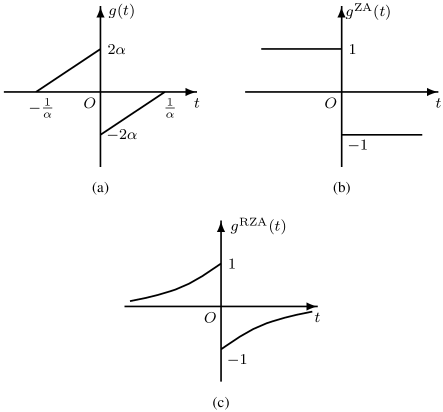
Figure 1: The Zero-point attraction of (a) $l_{0}$-LMS, (b) ZA-LMS, (c) RZA-LMS.

2.3 Previous results on LMS and ZA-LMS

Denote $D^{\rm LMS}_{\infty}$ and $D^{\rm LMS}_{n}$ as the steady-state MSD and instantaneous MSD after $n$ iterations for LMS with zero-mean independent Gaussian input, respectively. The steady-state MSD has the explicit expression [2] of

$$D^{\rm LMS}_{\infty}=\frac{\mu P_{v}L}{2-\mu P_{x}(L+2)}=\frac{\mu P_{v}L}{\Delta_{L}},$$ (8)

where $P_{x}$ and $P_{v}$ denote the power of input signal and additive noise, respectively, and $\Delta_{L}$ is a constant defined by (25) in Appendix A. For the convergence process, the explicit expression of instantaneous MSD is implied in [36] as

$$D^{\rm LMS}_{n}=\frac{\mu P_{v}L}{\Delta_{L}}+\left(\|{\bf s}\|_{2}^{2}-\frac{\mu P_{v}L}{\Delta_{L}}\right)\cdot\left(1-\mu P_{x}\Delta_{L}\right)^{n}.$$ (9)

The next one turns to ZA-LMS, $D^{\rm ZA}_{\infty}$ is used to denote the steady-state MSD with white Gaussian input. Reference [46] reaches the conclusion that

$$D^{\rm ZA}_{\infty}=\frac{2}{\mu P_{x}}\left(y^{2}-\frac{\pi\mu P_{x}+\Delta_{0}}{2\pi\mu^{2}P_{x}^{2}}\rho^{2}\right)-\frac{P_{v}}{P_{x}},$$ (10)

where $y$ is the solution to

$$\Delta_{L}y^{2}+(L-Q)\rho\sqrt{\frac{2\Delta_{0}}{\pi}}y-\left(\frac{L-2Q}{2\pi}+Q+1\right)\frac{\Delta_{0}\rho^{2}}{\mu P_{x}}-\frac{\Delta_{0}^{2}\rho^{2}}{\pi\mu^{2}P_{x}^{2}}-\mu P_{v}\Delta_{0}=0,$$

where $Q\leq L$ denotes the number of non-zero unknown coefficients and $\Delta_{0}$ is a constant defined by (27).

2.4 Related steepest ascent algorithms for sparse decomposition

$l_{0}$-LMS employs steepest descent recursively and is applicable to solving sparse system identification. More generally, steepest ascent iterations are used in several algorithms in the field of sparse signal processing. For example, researchers developed smoothed $l_{0}$ method [24] for sparse decomposition, whose iteration includes a steepest ascent step and a projection step. The first step is defined as

$${\bf\hat{w}}_{n+1}={\bf w}_{n}+\mu{\mathbf{v}}^{\rm SL0}_{n},$$ (11)

where $\mu$ serves as step size, ${\mathbf{v}}^{\rm SL0}_{n}=[v^{\rm SL0}_{0,n},v^{\rm SL0}_{1,n},...,v^{\rm SL0}_{L-1,n}]^{\rm T}$ denotes the negative derivative to an approximated $l_{0}$ norm and takes the value

$$v^{\rm SL0}_{k,n}=-w_{k,n}{\rm exp}\left(-2w_{k,n}^{2}/\sigma^{2}\right),\ \ 0\leq k<L.$$

After (11), a projection step is performed which maps ${\bf\hat{w}}_{n+1}$ to ${\bf w}_{n+1}$ in the feasible set. It can be seen that (11) performs steepest ascent, which is similar to zero-point attraction in $l_{0}$-LMS. The iteration details and performance analysis of this algorithm are presented in [24] and [25], respectively.

Another algorithm, named Iterative Bayesian[26], also enjoys steepest ascent iteration as

$${\bf w}_{n+1}={\bf w}_{n}+\mu\frac{\partial L}{\partial{\bf w}},$$ (12)

where $\mu$ denotes the step size and $L$ is a log posterior probability function. Analysis of this algorithm and its application to sparse component analysis in noisy scenario are presented in [26].

3 Preliminaries

Considering the nonlinearity of zero-point attraction, some preparations are made to simplify the mean square performance analysis.

3.1 Classification of unknown coefficients

Because various affects are exerted in $l_{0}$-LMS to the filter tap-weights according to their respective system coefficients, it would be helpful to classify the unknown parameters, correspondingly, the filter tap-weights, into several categories and perform different analysis on each category separately. According to the attraction range and their strength, all system coefficients are classified into three categories as

$${\rm Large\ coefficients}: \mathcal{C}_{L}=\left\{k{\big{|}}|s_{k}|\geq 1/\alpha\right\};$$

$${\rm Small\ coefficients}: \mathcal{C}_{S}=\left\{k{\big{|}}0<|s_{k}|<1/\alpha\right\};$$

$${\rm Zero\ coefficients}: \mathcal{C}_{0}=\left\{k{\big{|}}s_{k}=0\right\},$$

where $0\leq k<L$. Obviously, $|\mathcal{C}_{L}\cup\mathcal{C}_{S}\cup\mathcal{C}_{0}|=L$ and $|\mathcal{C}_{L}\cup\mathcal{C}_{S}|=Q$. In the following text, derivations are firstly carried out for the three sets separately. Then a synthesis is taken to achieve the final results.

3.2 Basic assumptions

The following assumptions about the system and the predefined parameters are adopted to enable the formulation.

• Input data $x(n)$ is an i.i.d. zero-mean Gaussian signal.

• Tap-weights ${\bf w}_{n}$, input vector ${\bf x}_{n}$, and additive noise $v_{n}$ are mutually independent.

• The parameter $\kappa$ is so small that $2\alpha^{2}\kappa\ll\mu P_{x}$.

Assumption (i) commonly holds while (ii) is the well-known independence assumption [3]. Assumption (iii) comes from the experimental observations, i.e., a too large $\kappa$ can cause much bias as well as large steady-state MSD. Therefore, in order to achieve better performance, $\kappa$ should not be too large.

Besides the above items, several regular patterns are supposed during the convergence and the steady state.

• All tap-weights, ${\bf w}_{n}$, follow Gaussian distribution.

• For $k\in\mathcal{C}_{L}\bigcup\mathcal{C}_{S}$, the tap-weight $w_{k,n}$ is assumed to have the same sign with the corresponding unknown coefficient.

• The adaptive weight $w_{k,n}$ is assumed out of the attraction range for $k\in\mathcal{C}_{L}$, while in the attraction range elsewhere.

Assumption (iv) is usually accepted for steady-state behavior analysis [12, 49]. Assumption (v) and (vi) are considered suitable in this work due to the following two aspects. First, there are few taps violating these assumptions in a common scenario. Intuitively, only the non-zero taps with rather small absolute value may violate assumption (v), while assumption (vi) may not hold for the taps close to the boundaries of the attraction range. For other taps which make up the majority, these assumptions are usually reasonable, especially in high SNR cases. Second, assumptions (v) and (vi) are proper for small steady-state MSD, which is emphasized in this work. The smaller steady-state MSD is, the less tap-weights differ from unknown coefficients. Therefore, it is more likely that they share the same sign, as well as on the same side of the attraction range.

Based on the discussions above, those patterns are regarded suitable in steady state. For the convergence process, due to fast convergence of LMS-type algorithms, we may suppose that most taps will get close to the corresponding unknown coefficients very quickly, so these patterns are also employed in common scenarios. As we will see later, some of the above assumptions cannot always hold in whatever parameter setting and may restrict the applicability of some analysis below. However, considering the difficulties of nonlinear algorithm performance analysis, these assumptions can significantly enable mathematical tractability and help obtain results shown to be precious in a large range of parameter setting. Thus, we consider these assumptions reasonable to be employed in this work.

4 Performance analysis

Based on the assumptions above, the mean and mean-square performances of $l_{0}$-LMS are analyzed in this section.

4.1 Mean performance

Define the misalignment vector as ${\bf h}_{n}={\bf w}_{n}-{\bf s}$, combine (1), (2), and (3), one has

$${\bf h}_{n+1}=\left({\bf I}-\mu{\bf x}_{n}{\bf x}^{\rm T}_{n}\right){\bf h}_{n}+\mu v_{n}{\bf x}_{n}+\kappa g({\bf w}_{n}).$$ (13)

Taking expectation and using the assumption (ii), one derives

$$\overline{{\bf h}_{\infty}}=\frac{\kappa}{\mu P_{x}}\overline{g({\bf w}_{\infty})},$$

where overline denotes expectation.

• For $k\in\mathcal{C}_{L}$, utilizing assumption (vi), one has $\overline{g(w_{k,\infty})}=0$.

• For $k\in\mathcal{C}_{S}$, combining assumptions (iii), (v) and (vi), it can be derived that

  $$\overline{h_{k,\infty}}=\left(1-\frac{2\alpha^{2}\kappa}{\mu P_{x}}\right)\frac{\kappa g(s_{k})}{\mu P_{x}}\\ \approx\frac{\kappa g(s_{k})}{\mu P_{x}}.$$

• For $k\in\mathcal{C}_{0}$, noticing the fact that $g(x)$ has the opposite sign with $x$ in interval $(-1/\alpha,1/\alpha)$ and using assumptions (iv) and (vi), it can be derived that $\overline{g(w_{k,\infty})}=0$.

Thus, the bias in steady state is obtained

$$\overline{h_{k,\infty}}=\begin{cases}\frac{\kappa g(s_{k})}{\mu P_{x}}&k\in\mathcal{C}_{S};\\ 0&{\rm elsewhere}.\end{cases}$$ (14)

In steady state, therefore, the tap-weights are unbiased for large coefficients and zero coefficients, while they are biased for small coefficients. The misalignment depends on the predefined parameters as well as unknown coefficient $s_{k}$ itself. The smaller the unknown coefficient is, the larger the bias becomes. This tendency can be directly read from Fig. 1(a). In the attraction range, the intensity of the zero-point attraction increases as tap-weights get more closing to zero, which causes heavy bias. Thus, the bias of small coefficients in steady state is the byproduct of the attraction, which accelerates the convergence rate and increases steady-state MSD.

4.2 Mean square steady-state performance

The condition on mean square convergence and steady-state MSD are given by the following theorem.

Theorem 1

In order to guarantee convergence, step-size $\mu$ should satisfy

$$0<\mu<\mu_{\rm max}=\frac{2}{(L+2)P_{x}},$$ (15)

and the final mean square deviation of $l_{0}$-LMS is

$$D_{\infty}=\frac{\mu P_{v}L}{\Delta_{L}}+\beta_{1}\kappa^{2}-\beta_{2}\kappa\sqrt{\kappa^{2}+\beta_{3}},$$ (16)

where $\{\beta_{i}\}$ are defined in (36)$\sim$(38) in Appendix A, respectively.  

The proof of Theorem 1 goes in Appendix B.

Remark 1: The steady-state MSD of $l_{0}$-LMS is composed of two parts: the first item in (16) is exactly the steady-state MSD of standard LMS (8), while the latter two items compose an additional part caused by zero-point attraction. When $\kappa$ equals zero, $l_{0}$-LMS becomes the traditional LMS, and correspondingly the additional part vanishes. When the additional part is negative, $l_{0}$-LMS has smaller steady-state MSD and thus better steady-state performance over standard LMS. Consequently, it can be deduced that the condition on $\kappa$ to ensure $l_{0}$-LMS outperforms LMS in steady-state is

$$0<\kappa<\frac{\beta_{2}^{2}\beta_{3}}{\beta_{1}^{2}-\beta_{2}^{2}}.$$

Remark 2: According to Theorem 1, the following corollary on parameter $\kappa$ is derived.

Corollary 1

From the perspective of steady-state performance, the best choice for $\kappa$ is

$$\kappa_{\rm{opt}}=\frac{\sqrt{\beta_{3}}}{2}\left(\sqrt[4]{\frac{\beta_{1}+\beta_{2}}{\beta_{1}-\beta_{2}}}-\sqrt[4]{\frac{\beta_{1}-\beta_{2}}{\beta_{1}+\beta_{2}}}\right),$$ (17)

and the minimum steady-state MSD is

$$D^{\rm min}_{\infty}=\frac{\mu P_{v}L}{\Delta_{L}}+\frac{\beta_{3}}{2}\left(\sqrt{\beta_{1}^{2}-\beta_{2}^{2}}-\beta_{1}\right).$$ (18)

 

The proof of Corollary 1 is presented in Appendix C. Please notice that in (18), the first item is about standard LMS and the second one is negative when $Q$ is less than $L$. Therefore, the minimum steady-state MSD of $l_{0}$-LMS is less than that of standard LMS as long as the system is not totally non-sparse.

Remark 3: According to the theorem, it can be accepted that the steady-state MSD is not only controlled by the predefined parameters, but also dependent on the unknown system in the following two aspects. First, the sparsity of the system response, i.e. $Q$ and $L$, controls the steady-state MSD. Second, significantly different from standard LMS, the steady-state MSD is relevant to the small coefficients of the system, considering the attracting strength appears in $\beta_{0}$ and $\beta_{1}$.

Here we mainly discuss the effect of system sparsity as well as the distribution of coefficients on the minimum steady-state MSD. Based on the above results, the following corollary can be deduced.

Corollary 2

The minimum steady-state MSD of (18) is monotonic increasing with respect to $Q$ and attracting strength $G({\bf s})$.  

The validation of Corollary 2 is performed in Appendix D. The zero-point attractor is utilized in $l_{0}$-LMS to draw tap-weights towards zero. Consequently, the more sparse the unknown system is, the less steady-state MSD is. Similarly, small coefficients are biased in steady state and deteriorate the performance, which explains that steady-state MSD is increasing with respect to $G({\bf s})$.

Remark 4: According to (15), one knows that $l_{0}$-LMS has the same convergence condition on step size as standard LMS[2] and ZA-LMS[46]. Consequently the effect of $\mu$ on steady-state performance is analyzed. It is indicated in (8) that the standard LMS enhances steady-state performance by reducing step size[2]. $l_{0}$-LMS has a similar trend. For the seek of simplicity and practicability, a sparse system of $Q$ far less than $L$ is considered to demonstrate this property. Utilizing (15) in such scenario, the following corollary is derived.

Corollary 3

For a sparse system which satisfies

$$Q\ll L\quad{\rm and}\quad(Q+2)\mu P_{x}\ll 2,$$ (19)

the minimum steady-state MSD in (18) is further approximately simplified as

$$D^{\rm min}_{\infty}\approx\frac{\mu P_{v}L}{\Delta_{L}}\!\!\left(\!1\!-\!\frac{\eta_{6}}{\eta_{5}+\eta_{6}+\!\!\sqrt{\eta_{5}^{2}+\frac{32\alpha^{2}L}{\pi}G({\bf s})}}\right)\!\!,$$ (20)

where $\eta_{5}$ and $\eta_{6}$ are defined by (42) in Appendix A, and $G({\bf s})$, defined by (29), denotes the attracting strength to the zero-point. Furthermore, the minimum steady-state MSD increases with respect to the step size.  

The proof of Corollary 3 is conducted in Appendix E. Due to the stochastic gradient descent and zero-point attraction, the tap-weights suffer oscillation, even in steady state, whose intensity is directly relevant to the step size. The larger the step size, the more intense the vibration. Thus, the steady-state MSD is monotonic increasing with respect to $\mu$ in the above scenario.

Remark 5: In the scenario where $2\alpha\kappa=\rho$ remains a constant while $\alpha$ approaches to zero, it can be readily accepted that (3) becomes totally identical to (6), therefore $l_{0}$-LMS becomes ZA-LMS in this limit setting of parameters. In Appendix F it is shown that the result (10) for steady-state performance [12] could be regarded as a particular case of Theorem 1. As $\alpha$ approaches to zero in $l_{0}$-LMS, the attraction range becomes infinity and all non-zero taps belong to small coefficients which are biased in steady state. Thus, ZA-LMS has larger steady-state MSD than $l_{0}$-LMS, due to bias of all taps caused by uniform attraction intensity. If $\kappa$ is further chosen optimal, the optimal parameter for ZA-LMS is given by $\rho_{\rm{opt}}=\lim_{\alpha\rightarrow 0}2\alpha\kappa_{\rm{opt}}$ (notice that $\kappa_{\rm{opt}}$ approaches $\infty$ as $\alpha$ tending to zero, as makes $\rho_{\rm{opt}}$ finite), and the minimum steady-state MSD of $l_{0}$-LMS (18) converges to that of ZA-LMS. To better compare the three algorithms, the steady-state MSDs of LMS, ZA-LMS, and $l_{0}$-LMS are listed in TABLE 1, where that of ZA-LMS is rewritten and $\Gamma$ is defined in (64) in Appendix F. It can be accepted that the steady-state MSDs of both ZA-LMS and $l_{0}$-LMS are in the form of $D_{\infty}^{\rm LMS}$ plus addition items, where $D_{\infty}^{\rm LMS}$ denotes the steady-state MSD of standard LMS. If the additional items are negative, ZA-LMS and $l_{0}$-LMS exceed LMS in steady-state performance.

Table 1: The steady-state MSDs of three algorithms.

		Steady-state MSD
Alg.	Relat. w. $l_{0}$-LMS	Eq. No.	Denota.	Expression
$l_{0}$-LMS	—	(16)	$D_{\infty}$	$D^{\rm LMS}_{\infty}+\beta_{1}\kappa^{2}-\beta_{2}\kappa\sqrt{\kappa^{2}+\beta_{3}}$
ZA-LMS	$2\alpha\kappa\!=\!\rho\!$ and $\!\alpha\!\rightarrow\!0$	(63)	$D^{\rm ZA}_{\infty}$	$D^{\rm LMS}_{\infty}\!-\!\frac{\rho(L-Q)\sqrt{\Gamma}}{\sqrt{2\pi}\mu^{2}P_{x}^{2}\Delta_{L}^{2}}\!+\!\frac{\rho^{2}(2(L-Q)\Delta_{0}\Delta_{Q}+\pi\Delta_{L}(\mu LP_{x}+2Q\Delta_{0}))}{\pi\mu^{2}P_{x}^{2}\Delta_{L}^{2}}$
LMS	$\kappa=0$	(8)	$D^{\rm LMS}_{\infty}$	$\frac{\mu P_{v}L}{\Delta_{L}}$

Remark 6: Now the extreme case that all taps in system are zero, i.e. $Q=0$, is considered. If $\kappa$ is set as the optimal, (18) becomes

$$D_{\infty}^{\rm min}=\frac{\mu P_{v}L}{\Delta_{L}}-\frac{2\mu P_{v}L\Delta_{0}^{2}}{2\Delta_{L}\Delta_{0}^{2}+\pi\mu P_{x}\Delta_{L}^{2}}.$$ (21)

Due to the independence of (21) on $\alpha$, this result also holds in the scenario of $\alpha$ approaching zero; thus, (21) also applies for the steady-state MSD of ZA-LMS with optimal $\rho$, in the extreme case $Q=0$. Thus, it has been shown that $l_{0}$-LMS and ZA-LMS with respective optimal parameters have the same steady state performance for a system with all coefficients zero. Although this result seems a little strange at the first sight, it is in accordance with intuition considering the zero-point attraction item in $l_{0}$-LMS. Since the system only has zero taps, all $w_{k,\infty}$ only vibrate in a very small region around zero. The zero-point attraction item is $\kappa g(t)\approx-2\alpha\kappa{\rm sgn}(t)$ when $t$ is very near zero, thus as long as we set $\alpha\kappa$ to be constant, the item mentioned above and the steady state MSD have little dependence on $\alpha$ itself. Thus, when $\kappa$ is chosen as optimal and $Q=0$, the steady state MSD generally does not change with respect to $\alpha$.

4.3 Mean square convergence behavior

Based on the results achieved in steady state, the convergence process can be derived approximately.

Lemma 1

The instantaneous MSD is the solution to the first order difference equations

$$\left[\!\!\begin{array}[]{c}D_{n+1}\\ \Omega_{n+1}\end{array}\!\!\right]={\mathbf{A}}\left[\!\!\begin{array}[]{c}D_{n}\\ \Omega_{n}\end{array}\!\!\right]+{\mathbf{b}_{n}},$$ (22)

where $\Omega_{n}=\sum_{k\in\mathcal{C}_{0}}\overline{h^{2}_{k,n}}$, vector ${\bf b}_{n}$ and constant matrix ${\bf A}$ are defined in (32) and (31) in Appendix A, respectively. Initial values are

$$\left[\!\!\begin{array}[]{c}D_{0}\\ \Omega_{0}\end{array}\!\!\right]=\left[\!\!\begin{array}[]{c}\|{\bf s}\|_{2}^{2}\\ 0\end{array}\!\!\right].$$ (23)

 

The derivation of Lemma 1 goes in Appendix G. Since $\omega$, which is defined by (56), appears in both $\bf A$ and ${\bf b}_{n}$, the convergence process is affected by algorithm parameters, the length of system, the number of non-zero unknown coefficients, and the strength or distribution of small coefficients. Moreover, derivation in Appendix H yields the solution to (22) in the following theorem.

Theorem 2

The closed form of instantaneous MSD is

$$D_{n}=c_{1}\lambda_{1}^{n}+c_{2}\lambda_{2}^{n}+c_{3}\lambda_{3}^{n}+D_{\infty},$$ (24)

where $\lambda_{1}$ and $\lambda_{2}$ are the eigenvalues of matrix ${\mathbf{A}}$, $c_{1}$ and $c_{2}$ are coefficients defined by initial values (23). The expressions of constants $\lambda_{3}$ and $c_{3}$ are listed in (33) and (34) in Appendix A, respectively. $D_{\infty}$ denotes the steady-state MSD.  

The two eigenvalues can be easily calculated. Through the method of undetermined coefficients, $c_{1}$ and $c_{2}$ are obtained by satisfying initial values $D_{0}$ and $D_{1}$, which is acquired by (22) and (23). Considering the high complexity of their closed form expressions, they are not included in this paper for the sake of simplicity.

Next we discuss the relationship of mean square convergence between $l_{0}$-LMS and standard LMS. In the scenario where $l_{0}$-LMS with zero $\kappa$ becomes traditional LMS, it can be shown after some calculation that $c_{2}=c_{3}=0$ in (24), which becomes in accordance with (9). Now we turn to the MSD convergence rate of these two algorithms. From the perspective of step size, one has the following corollary.

Corollary 4

A sufficient condition for that $l_{0}$-LMS finally converges more quickly than LMS is $\mu_{\rm max}/2<\mu<\mu_{\rm max}$, where $\mu_{\rm max}$ is defined in (15).  

The proof is postponed to Appendix I. From Corollary 4, one knows that for a large step size, the convergence rate of $l_{0}$-LMS is finally faster than that of LMS. However, this condition is not necessary. In fact, $l_{0}$-LMS can also have faster convergence rate for small step size, as shown in numerical simulations.

On the perspective of the system coefficients distribution, one has another corollary.

Corollary 5

Another sufficient condition to ensure that $l_{0}$-LMS finally enjoys acceleration is

$$\mathcal{C}_{S}=\emptyset,\quad\text{or equivalently,}\quad\alpha\geq\max_{s_{k}\neq 0}\frac{1}{|s_{k}|}.$$

 

This corollary is obtained from the fact that $c_{3}$ equals zero in this condition, using the similar proof in Appendix I. The full demonstration is omitted to save space. Therefore, for sparse systems whose most coefficients are exactly zeros, a large enough $\alpha$ guarantees faster convergence rate finally. Similar as above, this condition is also not necessary. $l_{0}$-LMS can converge rather fast even if such condition is violated.

5 Numerical experiments

Five experiments are designed to confirm the theoretical analysis. The non-zero coefficients of the unknown system are Gaussian variables with zero mean and unit variance and their locations are randomly selected. Input signal and additive noise are white zero mean Gaussian series with various signal-to-noise ratio. Simulation results are the averaged deviation of $100$ independent trials. For theoretical calculation, the expectation of attracting strength in (29) and (30) are employed to avoid the dependence on priori knowledge of system. The parameters of these experiments are listed in TABLE 2, where $\kappa_{\rm opt}$ is calculated by (17).

Table 2: The parameters in experiments.

Experiment	$L$	$Q$	$\mu$	$\alpha$	$\kappa$	SNR
1	1000	100	$8$E$-4$	$10$	$1$E$-9\rightarrow 3$E$-6/1$E$-8\rightarrow 3$E$-5$	$40{\rm dB}/20{\rm dB}$
2	1000	100	$8$E$-4$	$5.6$E$-4\rightarrow 56$	$\kappa_{\rm opt}$	$40{\rm dB}$
3	1000	$50\rightarrow 1000$	$8$E$-4$	$10$	$\kappa_{\rm opt}$	$40{\rm dB}$
4	1000	100	$4$E$-4$	$10$	$0.1\kappa_{\rm opt}\rightarrow 10\kappa_{\rm opt}$	$40{\rm dB}/20{\rm dB}$
5	1000	100	$2$E$-4\rightarrow 4$E$-4$	$10$	$\kappa_{\rm opt}$	$40{\rm dB}$

In the first experiment, the steady-state performance with respect to $\kappa$ is considered. Referring to Fig. 2, the theoretical steady-state MSD of $l_{0}$-LMS is in good agreement with the experiment results when SNR is $40$dB. With the growth of $\kappa$ from $10^{-9}$, the steady-state MSD decreases at first, which means proper zero-point attraction is helpful for sufficiently reducing the amplitude of tap-weights in $\mathcal{C}_{0}$. On the other hand, larger $\kappa$ results in more intensity of zero-point attraction item and increases the bias of small coefficients $\mathcal{C}_{S}$. Overlarge $\kappa$ causes too much bias, thus deteriorates the overall performance. From (17), $\kappa_{\rm{opt}}=3.75\times 10^{-7}$ produces the minimized steady-state MSD, which is marked with a square in Fig. 2. Again, simulation result tallies with analytical value well. When SNR is $20$dB, referring to Fig. 3, the theoretical result also predicts the trend of MSD well. However, since the assumptions (v) and (vi) do not hold well in low SNR case, the theoretical result has perceptible deviation from the simulation result.

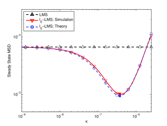
Figure 2: Steady-state MSD of LMS and $l_{0}$-LMS (with respect to different $\kappa$), where SNR is $40$dB and the solid square denotes $\kappa_{\rm opt}$.

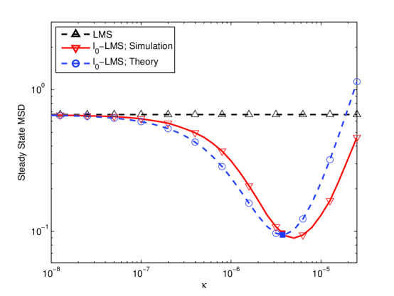
Figure 3: Steady-state MSD of LMS and $l_{0}$-LMS (with respect to different $\kappa$), where SNR is $20$dB and the solid square denotes $\kappa_{\rm opt}$.

In the second experiment, the effect of parameter $\alpha$ on steady-state performance is investigated. Please refer to Fig. 4 for results. RZA-LMS is also tested for performance comparison, with its parameter $\rho$ chosen as optimal values which are obtained by experiments. For the sake of simplicity, the parameter $\varepsilon$ in (7) is set the same as $\alpha$. Simulation results confirm the validity of the theoretical analysis. With very small $\alpha$, all tap-weights are attracted toward zero-point and the steady-state MSD is nearly independent. As $\alpha$ increases, there are a number of taps fall in the attraction range while the others are out of it. Consequently, the total bias reduces. Besides, the results for ZA-LMS are also considered in this experiment, with the optimal parameter $\rho$ proposed in Remark 5. It is shown that $l_{0}$-LMS always yields superior steady-state performance than ZA-LMS; moreover, in scenario where $\alpha$ approaches $0$, the MSD of $l_{0}$-LMS tends to that of ZA-LMS. In the parameter range of this experiment, $l_{0}$-LMS shows better steady-state performance than RZA-LMS.

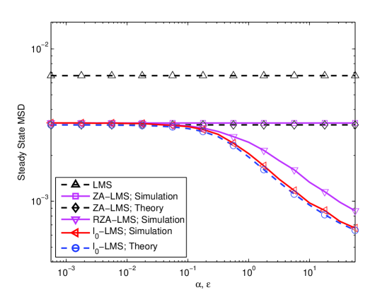
Figure 4: Steady-state MSD of LMS, ZA-LMS, RZA-LMS (with respect to different $\varepsilon$), and $l_{0}$-LMS (with respect to different $\alpha$), where $\varepsilon$ equals $\alpha$. Parameters $\rho$ and $\kappa$ are chosen as optimal for RZA-LMS and $l_{0}$-LMS, respectively.

The third experiment studies the effect of non-zero coefficients number on steady-state deviation. Please refer to Fig. 5. It is readily accepted that $l_{0}$-LMS with optimal $\kappa$ outperforms traditional LMS in steady state. The fewer the non-zero unknown coefficients are, the more effectively $l_{0}$-LMS draws tap-weights towards zero. Therefore, the effectiveness of $l_{0}$-LMS increases with the sparsity of the unknown system. When $Q$ exactly equals $L$, its performance with optimal $\kappa$ already attains that of standard LMS, indicating that there is no room for performance enhancement of $l_{0}$-LMS for a totally non-sparse system.

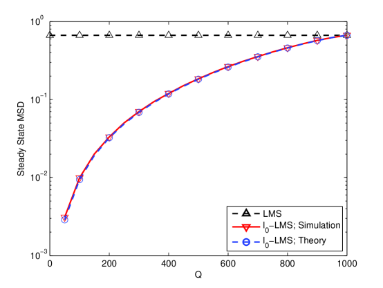
Figure 5: Steady-state MSD of LMS and $l_{0}$-LMS (with respect to different total non-zeros taps $Q$), where $\kappa$ is chosen as optimal.

The fourth experiment is designed to investigate convergence process with respect to $\kappa$. Also, the learning curve of the standard LMS is simulated. When SNR is $40$dB, the results in Fig. 6 demonstrate that our theoretical analysis of convergence process is generally in good accordance with simulation. It can be observed that different $\kappa$ results in differences in both steady-state MSD and the convergence rate. Due to more intense zero-attraction force, larger $\kappa$ results in higher convergence rate; but too large $\kappa$ can have bad steady-state performance for too much bias of small coefficients. Moreover, $l_{0}$-LMS outperforms standard LMS in convergence rate for all parameters we run, and also surpasses it in steady-state performance when $\kappa$ is not too large. When SNR is 20dB, Fig. 7 also shows similar trend about how $\kappa$ influences the convergence process; however, since the low SNR scenario breaks assumptions (v) and (vi), the theoretical results and experimental results differ to some extent.

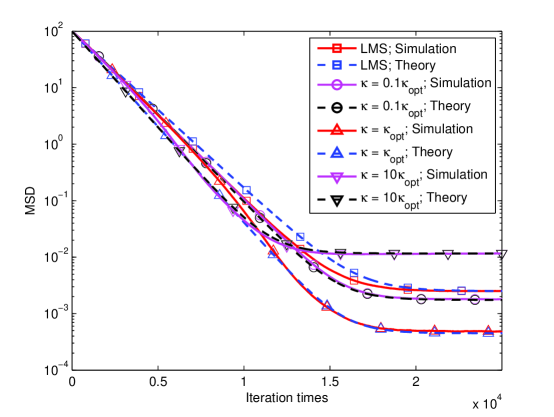
Figure 6: MSD convergence of LMS and $l_{0}$-LMS (with respect to different $\kappa$), where SNR is $40$dB.

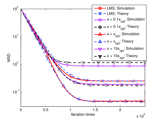
Figure 7: MSD convergence of LMS and $l_{0}$-LMS (with respect to different $\kappa$), where SNR is $20$dB.

The fifth experiment demonstrates convergence process for various step sizes, with the comparison of LMS and $l_{0}$-LMS. Please refer to Fig. 8. Similar to traditional LMS, smaller step size yields slower convergence rate and less steady-state MSD. Therefore, the choice of step size should seek a balance between convergence rate and steady-state performance. Furthermore, the convergence rate of $l_{0}$-LMS is faster than that of LMS when their step sizes are identical.

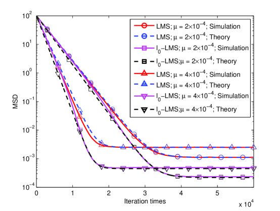
Figure 8: MSD convergence of LMS and $l_{0}$-LMS with respect to different step sizes $\mu$, where $\kappa$ is chosen as optimal for $l_{0}$-LMS.

6 Conclusion

The comprehensive mean square performance analysis of $l_{0}$-LMS algorithm is presented in this paper, including both steady-state and convergence process. The adaptive filtering taps are firstly classified into three categories based on the zero-point attraction item, and then analyzed separately. With the help of some assumptions which are reasonable in a wide range, the steady-state MSD is finally deduced and the convergence of instantaneous MSD is approximately predicted. Moreover, a parameter selection rule is put forward to minimize the steady-state MSD and theoretically it is shown that $l_{0}$-LMS with optimal parameters is superior than traditional LMS for sparse system identification. The all-round theoretical results are verified in a large range of parameter setting through numerical simulations.

Appendix A Expressions of constants

In order to make the main body simple and focused, the explicit expressions of some constants used in derivations are listed here.

All through this work, four constants of

$$\Delta_{L} =2-(L+2)\mu P_{x}$$ (25)

$$\Delta_{Q} =2-(Q+2)\mu P_{x}$$ (26)

$$\Delta_{0} =1-\mu P_{x}$$ (27)

$$\Delta^{\prime}_{0} =2-\mu P_{x}$$ (28)

are used to simplify the expressions.

To evaluate the zero-point attracting strength, with respect to the sparsity of the unknown system coefficients, two kinds of strengthes are defined as

$$G({\bf s}) =\left<g({\bf s}),g({\bf s})\right>=\sum\limits_{k\in\mathcal{C}_{S}}\!\!g^{2}(s_{k}),$$ (29)

$$G^{\prime}({\bf s}) =\left<{\bf s},g({\bf s})\right>=\sum\limits_{k\in\mathcal{C}_{S}}\!\!s_{k}g(s_{k}),$$ (30)

which are utilized everywhere in this work. Considering the attraction range, it can be readily accepted that these strengthes are only related to the small coefficients, other than the large ones and the zeros.

In Lemma 1, ${\bf A}=\left\{a_{ij}\right\}$ is defined as

$$\left[\!\!\begin{array}[]{cc}1-\mu P_{x}\Delta_{L}&-\sqrt{\frac{8}{\pi}}\frac{\alpha\kappa}{\omega}\Delta_{0}\\ (L-Q)\mu^{2}P_{x}^{2}&1\!-\!2\mu P_{x}\Delta_{0}\!-\!\sqrt{\frac{8}{\pi}}\frac{\alpha\kappa}{\omega}\Delta_{0}\end{array}\!\!\right],$$ (31)

and

$${{\bf b}_{n}}=[b_{0,n},b_{1,n}]^{\rm T},$$ (32)

where

$$b_{0,n}= L\mu^{2}P_{x}P_{v}+(L-Q)\left(4\alpha^{2}\kappa^{2}-\sqrt{8/\pi}\alpha\kappa\omega\Delta_{0}\right)$$

$$+\frac{\kappa^{2}(\Delta^{\prime}_{0}-2\Delta_{0}^{n+1})}{\mu P_{x}}G({\bf s})-2\kappa\Delta_{0}^{n+1}G^{\prime}({\bf s}),$$

$$b_{1,n}= (L-Q)\left(\mu^{2}P_{x}P_{v}+4\alpha^{2}\kappa^{2}-\sqrt{8/\pi}\alpha\kappa\omega\Delta_{0}\right),$$

where $\omega$ is the solution to (56).

In Theorem 2, the constants $\lambda_{3}$ and $c_{3}$ are

$$\lambda_{3}= \Delta_{0},$$ (33)

$$c_{3}= -\frac{2\kappa\Delta_{0}\left(\mu P_{x}-2\mu^{2}P_{x}^{2}+\sqrt{\frac{8}{\pi}}\frac{\alpha\kappa}{\omega}\Delta_{0}\right)}{\mu P_{x}\det\left(\lambda_{3}{\mathbf{I}}-{\mathbf{A}}\right)}\left(\kappa G({\bf s})+\mu P_{x}G^{\prime}({\bf s})\right).$$ (34)

In Corollary 1, the constants $\{\beta_{i}\}$ are

$$\beta_{0}= \mu P_{x}\Delta^{\prime}_{0}\Delta_{L}G({\bf s})+4\alpha^{2}\Delta_{Q}\left(\mu P_{x}\Delta_{L}+\frac{\Delta_{0}\Delta_{Q}}{\pi}\right),$$ (35)

$$\beta_{1}= \frac{\Delta^{\prime}_{0}G({\bf s})+4(L-Q)\alpha^{2}\left(\mu P_{x}+\frac{2\Delta_{0}\Delta_{Q}}{\pi\Delta_{L}}\right)}{\mu^{2}P_{x}^{2}\Delta_{L}},$$ (36)

$$\beta_{2}= \frac{4\alpha(L-Q)}{\mu^{2}P_{x}^{2}\Delta_{L}^{2}}\sqrt{\frac{\Delta_{0}\beta_{0}}{\pi}},$$ (37)

$$\beta_{3}= 2\mu^{3}P_{x}^{2}P_{v}\Delta_{0}\Delta_{L}/\beta_{0}.$$ (38)

In Appendix D and E, the constants $\{\eta_{i}\}$ are

$$\eta_{0}=\frac{16P_{v}\alpha^{2}\Delta_{0}^{2}}{\pi\mu P_{x}^{2}\Delta_{L}^{3}}, \eta_{1}=\frac{1}{\mu^{2}P_{x}^{2}\Delta_{L}},$$ (39)

$$\eta_{2}=\frac{(L-Q)\beta_{0}}{\Delta_{L}\Delta_{Q}}, \eta_{3}=\frac{4\alpha^{2}(L-Q)\Delta_{0}\Delta_{Q}}{\pi\Delta_{L}},$$ (40)

$$\eta_{4}=\frac{G({\bf s})\Delta^{\prime}_{0}\Delta_{L}}{\Delta_{Q}},$$ (41)

$$\eta_{5}=4\alpha^{2}P_{x}\mu+2G({\bf s})L, \eta_{6}=\frac{16\alpha^{2}L}{\pi\Delta_{L}}.$$ (42)

Appendix B Proof of Theorem 1

Proof 1

Denote $D_{n}$ to be MSD at iteration $n$, and ${\bf{R}}_{n}$ to be the second moment matrix of ${\bf h}_{n}$, respectively,

$$D_{n}= \overline{{\bf h}^{\rm{T}}_{n}{\bf h}_{n}},$$ (43)

$${\bf R}_{n}= \overline{{\bf h}_{n}{\bf h}^{\rm{T}}_{n}}.$$ (44)

Substituting (13) into (44), and expanding the term $\overline{{\bf x}_{n}{\bf x}^{\rm{T}}_{n}{\bf h}_{n}{\bf h}^{\rm{T}}_{n}{\bf x}_{n}{\bf x}^{\rm{T}}_{n}}$ into three second moments using the Gaussian moment factoring theorem [36], one knows

$${\bf R}_{n+1}= (1-2\mu P_{x}\Delta_{0}){\bf R}_{n}+\mu^{2}P_{x}^{2}\cdot{\rm{tr}}\left\{{\bf R}_{n}\right\}{\bf I}+\mu^{2}P_{x}P_{v}{\bf I}$$

$$+\kappa\Delta_{0}\overline{{\bf h}_{n}g({\bf w}^{\rm{T}}_{n})}+\kappa\Delta_{0}\overline{g({\bf w}_{n}){\bf h}_{n}^{\rm{T}}}+\kappa^{2}\overline{g({\bf w}_{n})g({\bf w}^{\rm{T}}_{n})}.$$ (45)

Using the fact that $D_{n}={\rm{tr}}\left\{{\bf R}_{n}\right\}$, one has

$$D_{n+1}=(1-\mu P_{x}\Delta_{L})D_{n}+L\mu^{2}P_{x}P_{v}+2\kappa\Delta_{0}\overline{{\bf h}^{\rm{T}}_{n}g({\bf w}_{n})}+\kappa^{2}\overline{\|g({\bf w}_{n})\|_{2}^{2}}.$$

Consequently, the condition needed to ensure convergence is $\left|1-\mu P_{x}\Delta_{L}\right|<1$ and (15) is derived directly, which is the same as standard LMS and similar with the conclusion in [27].

Next the steady-state MSD will be derived. Using (45) and considering the $k$th diagonal element, one knows

$$\overline{h^{2}_{k,\infty}}=\frac{\mu^{2}\!P_{x}^{2}\!D_{\infty}\!\!+\!\!\mu^{2}\!P_{x}\!P_{v}\!+\!2\kappa\Delta_{0}\overline{h_{k,\infty}g(w_{k,\infty})}\!\!+\!\!\kappa^{2}\overline{g^{2}(w_{k,\infty})}}{2\mu P_{x}\Delta_{0}}.$$ (46)

To develop $\overline{h^{2}_{k,\infty}}$, one should first investigate two items, namely $\overline{h_{k,\infty}g(w_{k,\infty})}$ and $\overline{g^{2}(w_{k,\infty})}$ in (46). For $k\in\mathcal{C}_{L}$, from assumption (vi) one knows $|w_{k,\infty}|>{1}/{\alpha}$, thus

$$\overline{h_{k,\infty}g(w_{k,\infty})}=\overline{g^{2}(w_{k,\infty})}=0.$$ (47)

For small coefficients, considering assumptions (v) and (vi), formula (4) implies $g(w_{k,\infty})$ is a locally linear function with slope $2\alpha^{2}$, which results in

$$g(w_{k,\infty})=g(s_{k})+2\alpha^{2}h_{k,\infty}.$$

Thus, it can be shown

$$\overline{h_{k,\infty}g(w_{k,\infty})} =2\alpha^{2}\overline{h^{2}_{k,\infty}}+g(s_{k})\overline{h_{k,\infty}},$$ (48)

$$\overline{g^{2}(w_{k,\infty})} =4\alpha^{4}\overline{h^{2}_{k,\infty}}+g^{2}(s_{k})+4\alpha^{2}g(s_{k})\overline{h_{k,\infty}},$$ (49)

where $\overline{h_{k,\infty}}$ is derived in (14).

Then turning to $k\in\mathcal{C}_{0}$, it is readily known that $h_{k,\infty}=w_{k,\infty}$ in this case. Thus, from assumptions (iv) and (vi), the following results can be derived from the property of Gaussian distribution,

$$\overline{h_{k,\infty}g(w_{k,\infty})} =2\alpha^{2}\overline{h^{2}_{k,\infty}}-2\alpha\overline{|h_{k,\infty}|}$$

$$=2\alpha^{2}\overline{h^{2}_{k,\infty}}-4\alpha\sqrt{\overline{h^{2}_{k,\infty}}}/\sqrt{2\pi},$$ (50)

$$\overline{g^{2}(w_{k,\infty})} =4\alpha^{4}\overline{h^{2}_{k,\infty}}-8\alpha^{3}\overline{|h_{k,\infty}|}+4\alpha^{2}$$

$$=4\alpha^{4}\overline{h^{2}_{k,\infty}}-16\alpha^{3}\sqrt{\overline{h^{2}_{k,\infty}}}/\sqrt{2\pi}+4\alpha^{2}.$$ (51)

Combining assumption (iii), (14) and (47)$\sim$(49), one can know the equivalency between (46) and following equations for $k$ in $\mathcal{C}_{L}$, $\mathcal{C}_{S}$, and $\mathcal{C}_{0}$, respectively,

$$2\mu P_{x}\Delta_{0}\overline{h^{2}_{k,\infty}}-\mu^{2}P_{x}^{2}D_{\infty}-\mu^{2}P_{x}P_{v} =0,\quad k\in\mathcal{C}_{L},$$ (52)

$$2\mu P_{x}\Delta_{0}\overline{h^{2}_{k,\infty}}-\mu^{2}P_{x}^{2}D_{\infty}-\mu^{2}P_{x}P_{v}-\kappa^{2}g^{2}(s_{k})\left(2/\mu/P_{x}-1\right) =0,\quad k\in\mathcal{C}_{S},$$ (53)

$$2\mu P_{x}\Delta_{0}\omega^{2}+8\alpha\kappa\Delta_{0}\omega/\sqrt{2\pi}-\mu^{2}P_{x}^{2}D_{\infty}-\mu^{2}P_{x}P_{v}-4\alpha^{2}\kappa^{2} =0,\quad k\in\mathcal{C}_{0},$$ (54)

where $\omega$ denotes $\sqrt{\overline{h^{2}_{k,\infty}}},k\in\mathcal{C}_{0}$ for simplicity. Summing (52) and (53) for all $k\in\mathcal{C}_{L}\bigcup\mathcal{C}_{S}$, and noticing that

$$\sum\limits_{k\in\mathcal{C}_{L}\bigcup\mathcal{C}_{S}}\overline{h^{2}_{k,\infty}}=D_{\infty}-(L-Q)\omega^{2},$$

it could be derived that

$$D_{\infty}=\frac{2(L-Q)\Delta_{0}}{\Delta_{Q}}\omega^{2}+\frac{Q\mu P_{v}}{\Delta_{Q}}+\frac{\kappa^{2}\Delta^{\prime}_{0}}{\mu^{2}P_{x}^{2}\Delta_{Q}}G({\bf s}),$$ (55)

where $G({\bf s})$ is introduced in (29). Combining (55) and (54), it can be reached that $\omega$ is defined by the following equation

$$2\mu P_{x}\Delta_{0}\Delta_{L}\omega^{2}+\frac{8\alpha\kappa\Delta_{0}\Delta_{Q}}{\sqrt{2\pi}}\omega-2\mu^{2}P_{x}P_{v}\Delta_{0}-4\alpha^{2}\kappa^{2}\Delta_{Q}-\kappa^{2}\Delta^{\prime}_{0}G({\bf s}) =0.$$ (56)

Finally, (16) is achieved after solving the quadratic equation above and a series of formula transformation on (55). Thus, the proof of Theorem 1 is completed.  

Appendix C Proof of Corollary 1

Proof 2

By defining $\theta=\arctan\left(\kappa/\sqrt{\beta_{3}}\right)$, (16) becomes

$$D_{\infty}=\mu P_{v}L/\Delta_{L}-\beta_{1}\beta_{3}+\beta_{3}\cdot f(\sin(\theta))/2,$$ (57)

where $f(x)$ is defined as

$$f(x)=\frac{\beta_{1}-\beta_{2}}{1-x}+\frac{\beta_{1}+\beta_{2}}{1+x},\quad x\in(0,1).$$

Next we want to find $x_{\rm{opt}}\in(0,1)$ which minimizes $f(x)$. Forcing the derivative of $f(x)$ with respect to $x$ to be zero, it can be obtained that

$$0<x_{\rm{opt}}=\frac{\sqrt{\beta_{1}+\beta_{2}}-\sqrt{\beta_{1}-\beta_{2}}}{\sqrt{\beta_{1}+\beta_{2}}+\sqrt{\beta_{1}-\beta_{2}}}<1.$$

Combining $\theta_{\rm{opt}}=\arcsin(x_{\rm{opt}})$ and substituting $\theta_{\rm{opt}}$ in (57), corollary 1 can be finally achieved.  

Appendix D Proof of Corollary 2

Proof 3

From (8), (18), (36), (37), and (39), it can be obtained that

$$D^{\rm min}_{\infty}=D^{\rm LMS}_{\infty}-\frac{\eta_{0}}{\frac{\beta_{1}}{(L-Q)^{2}}+\frac{\sqrt{\beta_{1}^{2}-\beta_{2}^{2}}}{(L-Q)^{2}}}.$$ (58)

Note neither the $D^{\rm LMS}_{\infty}$ defined in (8) nor $\eta_{0}$ defined in (39) is dependent on $Q$ or $G({\bf s})$, thus the focus of the proof is the denominator in (58). In the following, we will analyze the two items in the denominator separately and obtain their monotonicity. The first item in the denominator is

$$\frac{\beta_{1}}{(L-Q)^{2}}=\frac{1}{\mu^{2}P_{x}^{2}\Delta_{L}}\Bigg{(}\frac{\Delta^{\prime}_{0}}{(L-Q)^{2}}G({\bf s})+\frac{4\alpha^{2}}{L-Q}\left(\mu P_{x}+\frac{2\Delta_{0}}{\pi}\right)+\frac{8\alpha^{2}\mu P_{x}\Delta_{0}}{\pi\Delta_{L}}\Bigg{)},$$ (59)

From (59), it has already shown that $\beta_{1}/(L-Q)^{2}$ is increasing with respect to $Q$ and $G({\bf s})$. Next we consider the second item. It can be obtained beforehand that $\beta_{1}$ and $\beta_{2}$ equal $\eta_{1}\left(\eta_{2}+\eta_{3}+\eta_{4}\right)$ and $2\eta_{1}\sqrt{\eta_{2}\eta_{3}}$, respectively. Thus, one has

$$\frac{\sqrt{\beta_{1}^{2}-\beta_{2}^{2}}}{(L-Q)^{2}}=\eta_{1}\sqrt{\frac{\eta_{4}^{2}+2\eta_{4}(\eta_{2}+\eta_{3})+(\eta_{2}-\eta_{3})^{2}}{(L-Q)^{4}}}.$$ (60)

Further notice that

$$\eta_{2}-\eta_{3}= \mu P_{x}(L-Q)\left(4\alpha^{2}+\frac{\Delta^{\prime}_{0}}{\Delta_{Q}}G({\bf s})\right),$$

$$\eta_{2}+\eta_{3}= 4(L-Q)\alpha^{2}\left(\mu P_{x}+\frac{2\Delta_{0}\Delta_{Q}}{\pi\Delta_{L}}\right)+\frac{\mu P_{x}(L-Q)\Delta^{\prime}_{0}}{\Delta_{Q}}G({\bf s}),$$

it can be proved that all of the three items in the square root of (60) are increasing with respect to $Q$ and $G({\bf s})$; thus the second item in the denominator is monotonic increasing with respect to $Q$ and $G({\bf s})$. Till now, the monotonicity of $D^{\rm min}_{\infty}$ with respect to $Q$ and $G({\bf s})$ has been proved. Last, in the special scenario where $Q$ exactly equals $L$, it can be obtained that $D^{\rm min}_{\infty}$ is identical to $D^{\rm LMS}_{\infty}$; thus $D^{\rm LMS}_{\infty}$ is larger than the minimum steady-state MSD of the scenario where $Q$ is less than $L$. In sum, Corollary 2 is proved.  

Appendix E Proof of Corollary 3

Proof 4

For a sparse system in accordance with (19), $\{\eta_{i}\}$ defined in Appendix A are approximated by

$$\eta_{0}\approx\frac{16P_{v}\alpha^{2}}{\pi\mu P_{x}^{2}\Delta_{L}^{3}}, \eta_{2}\approx\frac{8\alpha^{2}L}{\pi\Delta_{L}}+L\mu P_{x}G({\bf s})+4\alpha^{2}\mu P_{x}L,$$

$$\eta_{3}\approx\frac{8\alpha^{2}L}{\pi\Delta_{L}}, \eta_{4}\approx\Delta_{L}G({\bf s}).$$

Substituting $\{\eta_{i}\}$ in $\{\beta_{i}\}$ of (58), with the approximated expressions above, (20) is finally derived after calculation. Next we show $D^{\rm min}_{\infty}$ in (20) is monotonic increasing with respect to $\mu$. Since (20) is equivalent with

$$D^{\rm min}_{\infty}\!\!\approx\!\!\frac{P_{v}L\left(\eta_{5}+\sqrt{\eta_{5}^{2}+\frac{32\alpha^{2}L}{\pi}G({\bf s})}\right)}{\frac{16\alpha^{2}L}{\pi\mu}\!+\!\Delta_{L}\!\!\left(\!\!\frac{\eta_{5}}{\mu}\!+\!\!\sqrt{\left(\frac{\eta_{5}}{\mu}\right)^{2}\!\!\!+\!\!\frac{32\alpha^{2}L}{\pi\mu^{2}}G({\bf s})}\right)}.$$ (61)

it can be directly observed from (42) that larger $\mu$ results in larger numerator as well as smaller denominator in (61), which both contribute to the fact that $D^{\rm min}_{\infty}$ is monotonic increasing with respect to $\mu$. Thus, the proof of Corollary 3 is arrived.  

Appendix F Relationship with ZA-LMS

When $2\alpha\kappa=\rho$ remains a constant while $\alpha$ approaches zero, from (3), (4), and (5), it is obvious that the recursion of $l_{0}$-LMS becomes that of ZA-LMS. Furthermore, one can see that $g^{2}(x)$ equals $4\alpha^{2}+o(\alpha^{2})$. From the definition, it can be shown $\mathcal{C}_{L}$ is an empty set when $\alpha$ approaching zero. Consequently,

$$G({\bf s})=|\mathcal{C}_{S}|\cdot(4\alpha^{2}+o(\alpha^{2}))=4\alpha^{2}Q+o(\alpha^{2}).$$ (62)

Combine (55), (56), and (62), then after quite a series of calculation, the explicit expression of steady-state MSD becomes

$$D^{\rm ZA}_{\infty}= -\frac{(L-Q)\rho\sqrt{\Gamma}}{\sqrt{2\pi}\mu^{2}P_{x}^{2}\Delta_{L}^{2}}+\frac{2\rho^{2}(L-Q)\Delta_{0}\Delta_{Q}}{\pi\mu^{2}P_{x}^{2}\Delta_{L}^{2}}+\frac{\rho^{2}\left(\mu LP_{x}+2Q\Delta_{0}\right)+L\mu^{3}P_{x}^{2}P_{v}}{\mu^{2}P_{x}^{2}\Delta_{L}},$$ (63)

where $\Gamma$ is the discriminant of quadratic equation (56),

$$\Gamma=8\rho^{2}\Delta_{Q}^{2}\Delta_{0}^{2}/\pi+16\mu P_{x}\Delta_{L}\Delta_{0}^{2}\left(\rho^{2}(Q+1)+\mu^{2}P_{x}P_{v}\right).$$ (64)

Through a series of calculation, it can be proved that (63) is equivalent with (10) obtained in [46]. Thus, the steady-state MSD in ZA-LMS could be regarded as a particular case of that in $l_{0}$-LMS.

Appendix G Proof of Lemma 1

Proof 5

From (45), the update formula is

$$\overline{h^{2}_{k,n+1}}= (1-2\mu P_{x}\Delta_{0})\overline{h^{2}_{k,n}}+\mu^{2}P_{x}^{2}D_{n}+\mu^{2}P_{x}P_{v}+2\kappa\Delta_{0}\overline{h_{k,n}g(w_{k,n})}+\kappa^{2}\overline{g^{2}(w_{k,n})}.$$ (65)

Since LMS algorithm has fast convergence rate, it is reasonable to suppose most filter tap-weights will get close to the corresponding system coefficient very quickly; thus, the classification of coefficients $s_{k}$ could help in the derivation of the convergence situation of $h_{k,n}$.

For $k\in\mathcal{C}_{L}$, from assumption (vi), (65) takes the form

$$\overline{h^{2}_{k,n+1}}=(1-2\mu P_{x}\Delta_{0})\overline{h^{2}_{k,n}}+\mu^{2}P_{x}^{2}D_{n}+\mu^{2}P_{x}P_{v},k\in\mathcal{C}_{L}.$$ (66)

For $k\in\mathcal{C}_{S}$ the mean convergence is firstly derived and then the mean square convergence is deduced. Take expectation in (13), and combine assumptions (iii), (v), and (vi), one knows

$$\overline{h_{k,n+1}}=\Delta_{0}\overline{h_{k,n}}+\kappa g(s_{k}),k\in\mathcal{C}_{S}.$$

Since $h_{k}(0)=-s_{k}$, one can finally get

$$\overline{h_{k,n}}=\frac{\kappa g(s_{k})}{\mu P_{x}}-\frac{\mu P_{x}s_{k}+\kappa g(s_{k})}{\mu P_{x}}\Delta_{0}^{n},k\in\mathcal{C}_{S}.$$ (67)

Combining (65) , (67) and employing assumption (iii), it can be achieved

$$\ \overline{h^{2}_{k,n+1}}= (1-2\mu P_{x}\Delta_{0})\overline{h^{2}_{k,n}}+\mu^{2}P_{x}^{2}D_{n}+\mu^{2}P_{x}P_{v}+2\kappa\Delta_{0}g(s_{k})\overline{h_{k,n}}+\kappa^{2}g^{2}(s_{k}),k\in\mathcal{C}_{S}.$$ (68)

Next turn to $k\in\mathcal{C}_{0}$. From assumption (iv), the following formula can be attained employing the steady state result and first-order Taylor expansion

$$\overline{\left|h_{k,n}\right|}=\sqrt{2\overline{h^{2}_{k,n}}/\pi}\approx\left(\overline{h^{2}_{k,n}}/\omega+\omega\right)/\sqrt{2\pi},k\in\mathcal{C}_{0},$$

where $\omega=\sqrt{\overline{h^{2}_{k,\infty}}},k\in\mathcal{C}_{0}$, which is the solution to equation (56). Finally, with assumption (iii) we have

$$\ \overline{h^{2}_{k,n+1}}= \left(1-2\mu P_{x}\Delta_{0}-\sqrt{\frac{8}{\pi}}\frac{\alpha\kappa}{\omega}\Delta_{0}\right)\overline{h^{2}_{k,n}}+\mu^{2}P_{x}^{2}D_{n}$$

$$+\mu^{2}P_{x}P_{v}+4\alpha^{2}\kappa^{2}-\sqrt{\frac{8}{\pi}}\alpha\kappa\omega\Delta_{0},k\in\mathcal{C}_{0}.$$ (69)

Considering $\Omega_{n}=\sum_{k\in\mathcal{C}_{0}}\overline{h^{2}_{k,n}}$, and combine (66),(67),(68), and (69), one can obtain (22) after a series of derivation. As for the initial value, since $\mathbf{w}_{0}=0$, by definition we have $D_{0}=\|{\bf s}\|_{2}^{2}$ and $\Omega_{0}=0$. Thus, Lemma 1 is reached.  

Appendix H Proof of Theorem 2

Proof 6

The vector $\mathbf{b}_{n}$ in (32) could be denoted as

$${\mathbf{b}}_{n}=\left[\!\!\begin{array}[]{c}\hat{b}_{00}+\widehat{b}_{01}\lambda_{3}^{n}\\ \widehat{b}_{1}\end{array}\!\!\right],$$ (70)

where $\lambda_{3}$ is defined in (33) and $\widehat{b}_{00},\widehat{b}_{01},\widehat{b}_{1}$ are constants. Take $z$-Transform for (22), it can be derived that

$$\left[\!\!\!\begin{array}[]{c}D(z)\\ \Omega(z)\end{array}\!\!\!\right]=(z\mathbf{I}-\mathbf{A})^{-1}z\left[\!\!\!\begin{array}[]{c}D_{0}\\ \Omega_{0}\end{array}\!\!\!\right]+(z\mathbf{I}-\mathbf{A})^{-1}{\mathbf{b}(z)},$$

where $z>1$. Then combine the definition of $\{\lambda_{i}\}$ in Theorem 2 and the above results, it is further derived

$$D(z)=\sum_{i=0}^{3}\frac{c_{i}}{1-\lambda_{i}z^{-1}},$$

where $\lambda_{0}=1$ and $\{c_{i}\}$ are constants. Take the inverse $z$-Transform and notice the definition of $D_{\infty}$, it finally yields

$$D_{n}=D_{\infty}+c_{1}\lambda_{1}^{n}+c_{2}\lambda_{2}^{n}+c_{3}\lambda_{3}^{n}.$$

Thus we have completed the proof of (24). By forcing the equivalence between (24) and Lemma 1, the expression of $c_{3}$ could be solved as (34).  

Appendix I Proof of Corollary 4

Proof 7

Define function

$$p(x)=\det\left|x{\mathbf{I}}-{\mathbf{A}}\right|,\ x\in\mathbb{R},$$

then the roots of $p(x)$ are eigenvalues of matrix $\mathbf{A}$. From (31), it can be shown

$$\det\left|a_{00}{\mathbf{I}}-{\mathbf{A}}\right|=\det\left|a_{11}{\mathbf{I}}-{\mathbf{A}}\right|=-a_{01}a_{10}>0,$$

and

$$\det\left|\frac{a_{00}+a_{11}}{2}{\mathbf{I}}-{\mathbf{A}}\right|\leq-\frac{1}{4}\left(L\mu^{2}P_{x}^{2}-\sqrt{\frac{8}{\pi}}\frac{\alpha\kappa}{\omega}\Delta_{0}\right)^{2}\leq 0,$$

where $\{a_{ij}\}$ denote the entries of $\bf A$. Thus, we know $p(a_{11})>0$ and $p\left(\frac{a_{00}+a_{11}}{2}\right)\leq 0$, which indicates that one root of quadratic function $p(x)$ is within the interval $\left(a_{11},\frac{a_{00}+a_{11}}{2}\right]$. Similarly, another root of $p(x)$ is in $\left[\frac{a_{00}+a_{11}}{2},a_{00}\right)$. Thus, it can be concluded that the eigenvalues of $\mathbf{A}$ are both in $\mathbb{R}$ and satisfy

$$a_{11}<\lambda_{1}\leq\frac{a_{00}+a_{11}}{2}\leq\lambda_{2}<a_{00}=1-\mu P_{x}\Delta_{L}.$$ (71)

For large step size scenario of $1<\mu(L+2)P_{x}<2$, (33) and (71) yield

$$\max\left\{\lambda_{1},\lambda_{2},\lambda_{3}\right\}<1-\mu P_{x}\Delta_{L}.$$

Through comparison between (24) and (9), one can know for large $\mu$, all the three transient items in MSD convergence of $l_{0}$-LMS has faster attenuation rate than LMS, leading to acceleration of convergence rate.

References

• [1] B. Widrow and S. D. Stearns, Adaptive Signal Processing. Englewood Cliffs, NJ: Prentice-Hall, 1985.
• [2] S. Haykin, Adaptive Filter Theory. Englewood Cliffs, NJ: Prentice-Hall, 1986.
• [3] A. H. Sayed, Adaptive Filters. John Wiley $\&$ Sons, NJ, 2008.
• [4] G. Glentis, K. Berberidis, and S. Theodoridis, โ€œEfficient least squares adaptive algorithms for FIR transversal filtering,โ€ IEEE Signal Process. Mag., vol. 16, no. 4, pp. 13-41, Jul. 1999.
• [5] D. L. Duttweiler, โ€œProportionate normalized least-mean-squares adaptation in echo cancellers,โ€ IEEE Trans. Speech Audio Process., vol. 8, no. 5, pp. 508-518, Sept. 2000.
• [6] W. F. Schreiber, โ€œAdvanced television systems for terrestrial broadcasting: Some problems and some proposed solutions,โ€ Proc. IEEE, vol. 83, no. 6, pp. 958-981, Jun. 1995.
• [7] M. Abadi and J. Husoy, โ€œMean-square performance of the family of adaptive filters with selective partial updates,โ€ Signal Processing, vol. 88, no. 8, pp. 2008-2018, Aug. 2008.
• [8] M. Godavarti and A. O. Hero, โ€œPartial update LMS algorithms,โ€ IEEE Trans. Signal Process., vol. 53, no. 7, pp. 2382-2399, Jul. 2005.
• [9] H. Deng and R. A. Dyba, โ€œPartial update PNLMS algorithm for network echo cancellation,โ€ ICASSP, pp. 1329-1332, Taiwan, Apr. 2009.
• [10] R. K. Martin, W. A. Sethares, R. C. Williamson, and C. R. J. Jr., โ€œExploiting sparsity in adaptive filters,โ€ IEEE Trans. Signal Process., vol. 50, no. 8, pp. 1883-1894, Aug. 2002.
• [11] B. D. Rao and B. Song, โ€œAdaptive filtering algorithms for promoting sparsity,โ€ ICASSP, pp. 361-364, Jun. 2003.
• [12] Y. Chen, Y. Gu, and A. O. Hero, โ€œSparse LMS for system identification,โ€ ICASSP, pp. 3125-3128, Taiwan, Apr. 2009.
• [13] Y. Gu, J. Jin, and S. Mei, โ€œl0subscript๐‘™0l_{0} Norm constraint LMS algorithm for sparse system identification,โ€ IEEE Signal Process. Lett., vol. 16, no. 9, pp. 774-777, Sep. 2009.
• [14] B. Babadi, N. Kalouptsidis, and V. Tarokh, โ€œSPARLS: the sparse RLS algorithm,โ€ IEEE Trans. Signal Process., vol. 58, no. 8, pp. 4013-4025, Aug. 2010.
• [15] D. Angelosante, J. A. Bazerque, and G. B. Giannakis, โ€œOnline adaptive estimation of sparse signals: where RLS meets the $l_{1}$-norm,โ€ IEEE Trans. Signal Process., vol. 58, no. 7, pp. 3436-3447, Jul. 2010.
• [16] C. Paleologu, J. Benesty, and S. Ciochina, โ€œ An improved proportionate NLMS algorithm based on the $l_{0}$ norm ,โ€ ICASSP, pp. 309-312, Dallas, TX, Mar. 2010.
• [17] Y. Murakami, M. Yamagishi, M. Yukawa, and I. Yamada, โ€œA sparse adaptive filtering using time-varying soft-thresholding techniques,โ€ ICASSP, pp. 3734-3737, Dallas, TX, Mar. 2010.
• [18] G. Mileounis, B. Babadi, N. Kalouptsidis, and V. Tarokh, โ€œAn adaptive greedy algorithm with application to nonlinear communications,โ€ IEEE Trans. Signal Process., vol. 58, no. 6, pp. 2998-3007, Jun. 2010.
• [19] H. Zayyani, M. Babaie-Zadeh, and C. Jutten, โ€œCompressed sensing block MAP-LMS adaptive filter for sparse chennel estimation and a Bayesian Cramer-Rao bound,โ€ MLSP, Sep. 2009.
• [20] Y. Kopsinis, K. Slavakis, and S. Theodoridis, โ€œOnline sparse system identification and signal reconstruction using projections onto weighted $l_{1}$ balls,โ€ IEEE Trans. Signal Process., vol. 59, no. 3, pp. 905-930, Mar. 2011.
• [21] D. L. Donoho, โ€œCompressed sensing,โ€ IEEE Trans. Inf. Theory, vol. 52, no. 4, pp. 1289-1306, Apr. 2006.
• [22] E. Candรจs, J. Romberg, and T. Tao, โ€œRobust uncertainty principles: Exact signal reconstruction from highly incomplete frequency information,โ€ IEEE Trans. Inf. Theory, vol. 52, no. 2, pp. 489-509, Feb. 2006.
• [23] E. Candรจs, โ€œCompressive sampling,โ€ in Proc. Int. Congr. Math., vol. 3, pp. 1433-1452, Spain, Aug. 2006.
• [24] H. Mohimani, M. Babaie-Zadeh, and C. Jutten, โ€œA fast approach for overcomplete sparse decomposition based on smoothed L0 norm,โ€ IEEE Trans. Signal Process., vol.57, no.1, pp. 289-301, Jan. 2009.
• [25] H. Mohimani, M. Babaie-Zadeh, I. Gorodnitsky, and C. Jutten, โ€œSparse recovery using smoothed L0 (SL0): convergence analysis,โ€ submitted to IEEE Trans. Inf. Theorey.
• [26] H. Zayyani, M. Babaie-Zadeh, and C. Jutten, โ€œAn iterative Bayesian algorithm for sparse component analysis (SCA) in presence of noise,โ€ IEEE Trans. Signal Process., vol. 57, no. 10, pp. 4378-4390, Oct. 2009.
• [27] J. Jin, Y. Gu, and S. Mei, โ€œA stochastic gradient approach on compressive sensing signal reconstruction based on adaptive filtering framework,โ€ IEEE J. Sel. Topics Signal Process., vol. 4, no. 2, pp. 409-420, Apr. 2010.
• [28] C. Rich and W. Yin, โ€œIteratively reweighted algorithms for compressive sensing,โ€ ICASSP, pp. 3869-3872, Las Vegas, NV Apr. 2008.
• [29] S. Wright, R. Nowak, and M. Figueiredo,โ€œSparse reconstruction by separable approximation,โ€ ICASSP, pp. 3373-3376, Las Vegas, NV, Apr. 2008.
• [30] J. Tropp and A. Gilbert, โ€œSignal recovery from random measurements via orthogonal matching pursuit,โ€ IEEE Trans. Inf. Theory, vol. 53, no. 12, pp. 4655-4666, Dec. 2007.
• [31] K. Mayyas and T. Aboulnasr, โ€œLeaky LMS algorithm: MSE analysis for Gaussian data,โ€ IEEE Trans. Signal Process., vol. 45, no. 4, pp. 927-934, Apr. 1997.
• [32] K. Mayyas, โ€œPerformance analysis of the deficient length LMS adaptive algorithm,โ€ IEEE Trans. Signal Process., vol. 53, no. 8, pp. 2727-2734, Aug. 2005.
• [33] O. Dabeer and E. Masry, โ€œAnalysis of mean-square error and transient speed of the LMS adaptive algorithm,โ€ IEEE Trans. Inf. Theory, vol. 48, no. 7, pp. 1873-1894, Jul. 2002.
• [34] B. Widrow and M. E. Hoff, โ€œAdaptive switching circuits,โ€ IRE WESCON Convention Record, no. 4, pp. 96-104, 1960.
• [35] B. Widrow, J. M. McCool, M. C. Larimore and C. R. Johnson, โ€œStationary and nonstationary learning characteristics of the LMS adaptive filter,โ€ Proc. IEEE, vol. 64, no. 8, pp. 1151-1162, Aug. 1976.
• [36] L. Horowitz and K. Senne, โ€œPerformance advantage of complex LMS for controlling narrow-band adaptive arrays,โ€ IEEE Trans. Acoust., Speech, Signal Process., vol. ASSP-29, no. 3, pp. 722-736, Jun. 1981.
• [37] A. Feuer and E. Weinstein, โ€œConvergence analysis of LMS filters with uncorrelated Gaussian data,โ€ IEEE Trans. Acoust., Speech, Signal Process., vol. ASSP-33, no. 1, pp. 222-230, Feb. 1985.
• [38] S. K. Zhao, Z. H. Man, S. Y. Khoo, and H. R. Wu,โ€œStability and convergence analysis of transform-domain LMS adaptive filters with second-order autoregressive process,โ€ IEEE Trans. Signal Process., vol. 57, no. 1, pp. 119-130, Jan. 2009.
• [39] A. Ahlen, L. Lindbom, and M. Sternad, โ€œAnalysis of stability and performance of adaptation algorithms with time-invariant gains,โ€ IEEE Trans. Signal Process., vol. 52, no. 1, pp. 103-116, Jan. 2004.
• [40] S. C. Chan and Y. Zhou, โ€œConvergence behavior of NLMS algorithm for Gaussian inputs: solutions using generalized Abelian integral functions and step size selection,โ€ Journal of Signal Processing Systems, vol. 3, pp. 255-265, 2010.
• [41] D. T. M. Slock, โ€œOn the convergence behavior of the LMS and the normalized LMS algorithms,โ€ IEEE Trans. Signal Process., vol. 41, no. 9, pp. 2811-2825, Sept. 1993.
• [42] T. Y. Al-Naffouri and A. H. Sayed, โ€œTransient analysis of adaptive filters with error nonlinearities,โ€ IEEE Trans. Signal Process., vol. 51, no. 3, pp. 653-663, Mar. 2003.
• [43] B. Lin, R. X. He, L. M. Song, and B. S. Wang,โ€œSteady-state performance analysis for adaptive filters with error nonlinearities,โ€ ICASSP, pp. 3093-3096, Taiwan, Apr. 2009.
• [44] A. Zidouri, โ€œConvergence analysis of a mixed controlled $l_{2}-l_{p}$ adaptive algorithm,โ€ EURASIP Journal on Advances in Signal Processing, article ID. 893809, vol. 2010.
• [45] S. C. Chan and Y. Zhou, โ€œOn the performance analysis of the least mean M-estimate and normalized least mean M-estimate algorithms with Gaussian inputs and additive Gaussian and additive Gaussian and contaminated Gaussian noises,โ€ Journal of Signal Processing Systems, vol. 1, pp. 81-103, 2010.
• [46] K. Shi and P. Shi, โ€œConvergence analysis of sparse LMS algorithms with l1-norm penalty,โ€ Signal Processing, vol. 90, no. 12, pp. 3289-3293, Dec. 2010.
• [47] S. Dasgupta, C. R. Johnson, and A. M. Baksho, โ€œSign-sign LMS convergence with independent stochastic inputs,โ€ IEEE Trans. Inf. Theory, vol. 36, no. 1, pp. 197-201, Jan. 1990.
• [48] B. E. Jun, D. J. Park, and Y. W. Kim, โ€œConvergence analysis of sign-sign LMS algorithm for adaptive filters with correlated Gaussian data,โ€ ICASSP, pp. 1380-1383, Detroit, MI, May. 1995.
• [49] S. Koike, โ€œConvergence analysis of a data echo canceler with a stochastic gradient adaptive FIR filter using the sign algorithm,โ€ IEEE Trans. Signal Process., vol. 43, no. 12, pp. 2852-2861, Dec. 1995.
• [50] B. E. Jun and D. J. Park, โ€œPerformance analysis of sign-sign algorithm for transversal adaptive filters,โ€ Signal Process., vol. 62, no. 3, pp. 323-333, Nov. 1997.
• [51] G. Su, J. Jin, and Y. Gu, โ€œPerformance analysis of $l_{0}$-LMS with Gaussian input signal,โ€ International Conference on Signal Processing, pp. 235-238, Beijing, Oct. 2010.
• [52] J. Weston, A. Elisseeff, and B. Scholkopf, et al, โ€œUse of the zero norm with linear models and kernel methods,โ€ the Journal of Machine Learning Research, pp. 1439-1461, Mar. 2003.