Higgs boson production in high energy proton-nucleus collisions

Abstract

We study Higgs boson production from gluon-gluon fusion at mid-rapidity in high energy proton-nucleus collisions.For this process the presently still little known gluon distribution function $h_{1}^{\perp g}(x,k_{\perp})$ might give a numerically relevant contribution. We show by explicite calculation that using CGC (color glass condensate) model input the result obtained in the naive $k_{t}$ factorization approach matches the result obtained in the TMD factorization framework for a dilute medium. We also verify the earlier finding [14] that the $k_{t}$ factorization formalism for Higgs production breaks down in a dense medium. In doing so we formulate a hybrid model which allows one to treat such reactions theoretically.

1 Introduction

In recent years the theoretical understanding of transverse momentum dependent (TMD) parton distributions has made tremendous progress, up to the point that their further investigation can serve as one of the motivations for a new electron-ion collider [1]. Still there are many aspects which need further study. An especially interesting one is relevant for Higgs-production at the LHC. In this case it was realized that for $pp$ collisions in addition to the standard gluon contribution one gets a contribution proportional to a little known distribution function, usually refereed to as the distribution of linearly polarized gluons [2, 3] ($h_{1}^{\perp g}$ in the notation of Ref. [4]). Therefore, $h_{1}^{\perp g}$ has attracted a lot of attention recently. This new distribution function is the only spin dependent gluon TMD for an unpolarized nucleon/nucleus, and may be considered as the counterpart of the quark Boer-Mulders function $h_{1}^{\perp q}(x,k_{\perp})$ [5]. However, in contrast to the latter, $h_{1}^{\perp g}$ is time-reversal even implying that initial/final state interactions are not needed for its existence [6, 7]. This distribution function is of phenomenological interest, especially for small-$x$ physics at RHIC and LHC because a calculation in the saturation model [8] showed that its contributions are (at small-$x$) as large as those proportional to the unpolarized gluon distribution. Fortunately, it has been shown that $h_{1}^{\perp g}$ can be accessed, at least in principle, through measuring, e.g., azimuthal $\cos 2\phi$ asymmetries in processes such as jet or heavy quark pair production in electron-nucleon scattering as well as nucleon-nucleon scattering. Other promising observables are $\cos 2\phi$ asymmetries in photon pair production in hadron collisions [9, 10, 11]. Such measurements should be feasible at RHIC, the LHC, and a potential future Electron Ion Collider (EIC) [12, 1] and could play an important role to establish saturation effects. More recently, it has been found that the linearly polarized gluon distribution may affect the transverse momentum distribution of Higgs bosons produced from gluon fusion for $p_{H\perp}\ll m_{H}$, where $p_{H\perp}$ and $m_{H}$ are the Higgs transverse momentum and mass respectively [13, 14]. The authors of Ref. [13] proposed that the effect of linearly polarized gluons on the Higgs transverse momentum distribution can even be used, in principle, to determine the parity of the Higgs boson experimentally. Transverse momentum dependent factorization has been re-examined by taking into account the perturbative gluon-radiation correction to $h_{1}^{\perp g}$ [14]. The complete TMD factorization results for Higgs boson production are consistent with earlier findings based on the Collins-Soper-Sterman (CSS) formalism [17] and soft-collinear-effective theory [18]. Also, the transverse momentum resummation formalism applied to di-photon production in $pp$ collisions [19] is closely related.

Besides their obvious phenomenological interest, these investigations of Higgs production are also interesting from a more theoretical point of view. The theoretical description of transverse momentum dependent processes unavoidably includes gauge links in one or the other form. While the starting expressions for the different approaches look often quite different with respect to these gauge links, it turned out that quite often the resulting cross sections can be mapped onto one another in some approximation and for a suitable kinematic window. In the following we will discuss three such approaches, TMD factorization, $k_{t}$ factorization and a new hybrid approach.

TMD factorization
We will use the term TMD factorization in the sense of [20], which defines hard and soft factors, such that, e.g., the Higgs boson production cross section with $P_{\perp}\ll M$ reads [14]

$$\frac{d^{3}\sigma(M^{2},P_{\perp},y)}{d^{2}P_{\perp}dy} = \sigma_{0}\int d^{2}\vec{k}_{1\perp}d^{2}\vec{k}_{2\perp}d^{2}\vec{\ell}_{\perp}~{}\delta^{(2)}(\vec{k}_{1\perp}+\vec{k}_{2\perp}+\vec{\ell}_{\perp}-\vec{P}_{\perp})$$ (1)

$$\times \Bigl{\{}x_{1}g(x_{1},k_{1,\perp})~{}x_{2}g(x_{2},k_{2,\perp})~{}S(\ell_{\perp},\mu\rho)~{}H(M^{2},\mu\rho)$$

$$+ \left(\frac{2(k_{1\perp}\cdot k_{2\perp})^{2}}{k_{1\perp}^{2}k_{2\perp}^{2}}-1\right)~{}x_{1}h_{1}^{\perp g}(x_{1},k_{1,\perp})~{}x_{2}h_{1}^{\perp g}(x_{2},k_{2,\perp})$$

$$\times S_{h}(\ell_{\perp},\mu\rho)~{}H_{h}(M^{2},\mu\rho)\Bigr{\}}$$

with the soft factors $S$ and $S_{h}$ and the hard interaction factors $H$ and $H_{h}$. TMD factorization is probably the formally most complete and reliable scheme, but often also the calculational most demanding. For specific questions other schemes might be more economic. For example for all-order proofs of factorization SCET is a promising alternative [15] and for qualitative phenomenological analysis TMD factorization promisees a substantial simplification. Within TMD factorization there also exist different approaches. To be specific we use this term for the formulation of Collins et al. for which it is crucial to define the gauge links slightly off the light-cone. Within SCET it is possible to keep the gauge links on the light-cone [16]. In principle both approaches should give consistent results for physical observables when expanded in an appropriate manner, but it is non-trivial to map, e.g., evolution in both schemes onto one another.

$k_{t}$ factorization
In contrast, the naive $k_{t}$ factorization scheme invokes some approximations. In this formulation there is no linearly polarized gluon distribution function which is equivalent to the statement that it has to have the same functional form as the normal unpolarized gluon distribution such that it cannot be discerned. This fact demonstrates clearly that $k_{t}$ factorization can in general not be a good approximation because within CGC framework both gluon distributions could differ substantially for $Q_{s}\gg k_{\perp}$ as was first noticed in [8]. This can be best seen from the following expressions for the Weizsäcker-Williams (WW) unpolarized gluon distribution denoted by $G_{WW}(x,k_{\perp})$ and the WW type linearly polarized gluon distribution $h^{\perp g}_{1,WW}(x,k_{\perp})$ derived in the CGC formalism  [24, 25, 8],

$$xG_{WW}(x,k_{\perp})\!\!\! = \!\!\!\frac{N_{c}^{2}-1}{N_{c}}\frac{S_{\perp}}{4\pi^{4}\alpha_{s}}\int d^{2}r_{\perp}\,e^{-i\vec{k}_{\perp}\cdot\vec{r}_{\perp}}\,\frac{1}{r_{\perp}^{2}}\bigg{(}1-e^{-\frac{r_{\perp}^{2}Q_{s}^{2}}{4}}\bigg{)}\,,$$ (2)

$$xh^{\perp g}_{1,WW}(x,k_{\perp})\!\!\! = \!\!\!\frac{N_{c}^{2}-1}{8\pi^{3}}\,S_{\perp}\int dr_{\perp}\,\frac{J_{2}(k_{\perp}r_{\perp})}{\frac{1}{4\mu_{A}}r_{\perp}Q_{s}^{2}}\bigg{(}1-e^{-\frac{r_{\perp}^{2}Q_{s}^{2}}{4}}\bigg{)}\,.$$ (3)

Here $S_{\perp}$ is the transverse area of the target nucleus, and $k_{\perp}\equiv|\vec{k}_{\perp}|$. $Q_{s}^{2}=\alpha_{s}N_{c}\mu_{A}{\rm ln}\left[1/(r_{\perp}^{2}\Lambda_{QCD}^{2})\right]$ is the gluon saturation scale with $\mu_{A}$ being a common CGC parameter. Note that our convention for $h^{\perp g}_{1,WW}$ differs from that in Ref. [8] by a factor 1/2. In general, both gluon distributions are different though they become identical in the dilute region, i.e. for $k_{\perp}\gg Q_{s}$

hybrid approach
Our main strategy is to perform the calculations for proton-nucleus reactions in an approach where the nucleus is treated in the CGC framework  [28, 29, 30, 31], which effectively takes soft gluons into account, and the proton in the so-called Lipatov approximation  [32, 33, 34, 35]. We restrict ourself to studying Higgs production in the plain MV model [28] without considering small $x$ evolution effects although the latter could be done in principle [36, 37, 38, 39, 40, 41, 42] by solving the general JIMWLK evolution equation [43] for quadrupole operator. Neglecting evolution should be a good approximation because the MV model is valid in the range $x\approx 0.01-0.1$, which is the relevant kinematical regime for Higgs boson production at LHC, while radiative corrections only become important below a certain scale $x\approx 0.01$.

This article is organized as follows. In Sec. II, we introduce the hybrid approach and use it to reproduce the well known result for soft gluon production in $pA$ collisions. The Higgs boson production in $pA$ collisions is computed in the same approach in Sec III. We also demonstrate consistency between the results obtained in TMD factorization and $k_{t}$ factorization in the dilute region within the CGC model. We summary our paper in Sec. IV.

2 Soft gluon production in proton-nucleus collisions

In this section, we introduce a hybrid approach and reproduce the well known result for gluon production in high energy proton-nucleus scattering  [44, 45, 46, 47, 48, 49]. In the next section we shall generalize this approach to Higgs production. Let us first consider the general case of soft gluon production

$$A(P_{A})+p(P_{B})\rightarrow g(l)+X\ .$$ (4)

We assume that the nucleus is moving with a velocity very close to the speed of light into the positive $z$ direction, while the proton is moving in the opposite direction. It is convenient to use light-cone coordinates for which $P_{A}^{\mu}=P_{A}^{+}p^{\mu}$ and $P_{B}^{\mu}=P_{B}^{-}n^{\mu}$ with $p=(1,0,0,0)$ and $n=(0,1,0,0)$. The corresponding partonic subprocess is represented by $g_{A}(k_{1})+g_{p}(k_{2})\rightarrow g(l)$, where $k_{1}^{\mu}=x_{1}P_{A}^{+}p^{\mu}+k_{1\perp}^{\mu}$ denotes the total momentum carried by multiple gluons from the nucleus, and $k_{2}^{\mu}=x_{2}P_{B}^{-}n^{\mu}+k_{2\perp}^{\mu}$ is the momentum of the gluon from the proton. We chose to work in the light-cone gauge of the proton $(A^{-}=0)$, for which the polarization tensor of a produced gluon is given by,

$$\sum\epsilon^{\mu}\epsilon^{*\nu}=-g^{\mu\nu}+\frac{p^{\mu}l^{\nu}+p^{\nu}l^{\mu}}{p\cdot l}\ .$$ (5)

As mentioned above, to facilitate our calculation, a hybrid strategy has been adopted, in which the nucleus is treated in the CGC model, while on the side of the dilute projectile proton one makes the so-called Lipatov approximation [32, 33, 34, 35]. At small $x$ the gluon radiation cascade shows a strong ordering in rapidity. Or in other words, color source carries much larger rapidity than that radiated gluon does. It has been shown that a fast moving color source can be treated as eikonal line in the strongly rapidity ordered region. The operation of introducing these eikonal lines is refereed to as Lipatov approximation [35]. Its validity has been confirmed also by solving the classical Yang-Mills equation [47, 48, 49]. In these calculations, the gluon field induced inside a proton by a weak color source and weak color source itself are treated as a small parameter when solving classical Yang-Mills equation perturbatively. An analytic solution for the gauge field was obtained in lowest order of the incoming gluon field in various gauges [47, 48, 49].

For the process of gluon production in $pA$ collisions, the relevant eikonal line is the past-pointing one which is built up through initial state interactions between the color source inside the proton and the background gluon field. The interaction between the classical gluon field and the final state gluon emitted from the color source inside the proton does not change this general statement because the imaginary part of the scattering amplitude cancels between the different cut diagrams once the final states are integrated out. The prescription to treat the eikonal propagator is fixed by this choice. The relevant Feynman rules, illustrated in Fig. 1, were given in Ref. [35]. Note that the prescription for past-pointing eikonal propagators differs from that for future-pointing eikonal lines.

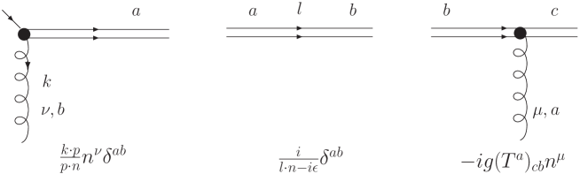
Figure 1: Feynman rules for the eikonal line, which is represented by a double line. $a,b,c$ denote color indices.

It is worthwhile to mention that to preserve gauge invariance one has to take both, gluon fusion and the interaction between the color source inside the proton and the strong classical gluon field of the large nucleus into account. This is due to the fact that the incoming gluon from the proton is off-shell and off-shell quantities are, in general, not gauge invariant. Both types of interaction are shown in Fig. 2.

The multiple scattering between incoming gluon (or eikonal line) and the classical color field of the nucleus can be readily resumed to all orders as has been done for the scattering of a quark by a background gluon field [51, 52]. The resumed multiple scattering gives rise to a path-ordered gauge factor along the straight line that extends in $x^{-}$ from minus infinity to plus infinity. More precisely, for a gluon or eikonal line with incoming momentum being $k$ and outgoing momentum being $k+q$, the path-ordered gauge factor reads,

$$2\pi\delta(q^{-})p^{\mu}[U-1](q_{\perp})\,,$$ (6)

with

$$[U-1](q_{\perp})=\int d^{2}x_{\perp}e^{-i\vec{q}_{\perp}\cdot\vec{x}_{\perp}}[U(x_{\perp})-1]\,,$$ (7)

and

$$U(x_{\perp})=\langle{\cal P}e^{-ig\int_{-\infty}^{+\infty}dx^{-}A^{+}(x^{-},\ x_{\perp})}\rangle_{A}\,,$$ (8)

where $A^{+}=A^{+}_{c}t^{c}$ is the gluon potential in the adjoint representation and $t^{c}_{ab}=-if_{abc}$ .

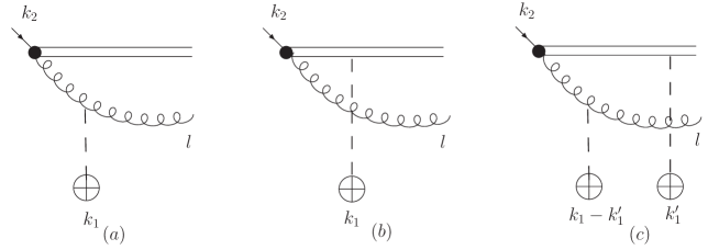
Figure 2: The diagrams contributing to gluon production. The dash lines represent the re-summed interactions of the incoming gluon or color source inside the proton with the classical color field of the nucleus.

We use this as a building block to compute the amplitude for gluon production in high energy $pA$ collisions. It is easy to verify that the contribution from the third diagram vanishes because both ${k_{1}^{\prime}}^{+}$ poles are located in the same half plane. Consequently, we are left with the contributions from the first two diagrams. The calculation of these two diagrams is straightforward. Collecting all pieces, the differential cross section reads,

$$\frac{d\sigma}{d^{2}ldy} = \frac{\pi}{(N_{c}^{2}-1)l_{\perp}^{2}}\int\frac{2d^{2}k_{1\perp}}{(2\pi)^{3}}k_{1\perp}^{2}x_{2}g(x_{2},k_{2\perp})[U-1](k_{1\perp})[U^{\dagger}-1](k_{1\perp})$$ (9)

$$= \frac{1}{(N_{c}^{2}-1)l_{\perp}^{2}}\int\frac{d^{2}k_{1\perp}}{(2\pi)^{2}}k_{1\perp}^{2}x_{2}g(x_{2},k_{2\perp})U(k_{1\perp})U^{\dagger}(k_{1\perp})\ ,$$

where $g(x_{2},k_{2\perp}\equiv|\vec{k}_{2\perp}|=|\vec{l}_{\perp}-\vec{k}_{1\perp}|)$ denotes the un-integrated gluon distribution of a proton, and $y$ is the rapidity of the produced gluon. The factor $2/(2\pi)^{3}$ associated with phase space integration is chosen such that for single gluon target, $\int\frac{2d^{2}k_{1\perp}}{(2\pi)^{3}}\frac{k_{1\perp}^{2}}{g^{2}N_{c}}\langle U(k_{1\perp})U^{\dagger}(k_{1\perp})\rangle_{\rm gluon}=x_{1}\delta(1-x_{1})$ at lowest non-trivial order (see, for example, Ref. [30]). To obtain the above result, we have defined the normalization factor and the flux factor to be $k_{2\perp}^{2}/(2k_{2}\cdot p(N_{c}^{2}-1))$ and $1/(2k_{2}\cdot p)$, respectively, rather than $k_{1\perp}^{2}k_{2\perp}^{2}/(4x_{1}x_{2}P_{A}\cdot P_{B}(N_{c}^{2}-1)^{2})$, $1/(4x_{1}x_{2}P_{A}\cdot P_{B})$ used in Ref. [35], since the Lipatov approximation is only justified for the proton side.

The next step is to compute the expectation value of a Wilson line in the plain McLerran-Venugopalan model [28]. By averaging over color sources with a Gaussian distribution, one finds [53, 54, 55],

$$\left\langle{\rm Tr}U(R_{\perp}+r_{\perp})U^{\dagger}(R_{\perp})\right\rangle_{A}=(N_{c}^{2}-1)\exp\left\{\frac{-Q_{s}^{2}r_{\perp}^{2}}{4}\right\}\ .$$ (10)

To proceed further, one notices that the dipole type gluon distribution in the adjoint representation is given by [46, 56, 57],

$$xG_{DP}(x,k_{\perp})=\frac{C_{F}S_{\perp}}{2\pi^{2}\alpha_{s}}k_{\perp}^{2}\int\frac{d^{2}r_{\perp}}{(2\pi)^{2}}\,e^{-i\vec{k}_{\perp}\cdot\vec{r}_{\perp}}\,e^{-\frac{Q_{s}^{2}r_{\perp}^{2}}{4}}\ .$$ (11)

With the help of the above two equations, the differential cross section can be written as,

$$\frac{d\sigma}{d^{2}ldy}=\frac{4\pi^{2}\alpha_{s}N_{c}}{(N_{c}^{2}-1)l_{\perp}^{2}}\int d^{2}k_{1\perp}x_{2}g(x_{2},k_{2\perp})x_{1}G_{DP}\left(x_{1},k_{1\perp}\right)\,$$ (12)

which is in full agreement with the results of earlier calculations  [44, 45, 46, 47, 48, 49, 50]. To see this, one has to identify $\pi x_{2}g(x_{2},k_{2\perp})\equiv\partial[x_{2}g(x_{2},Q^{2})]/\partial Q^{2}|_{Q^{2}=k_{2\perp}^{2}}$ and $\pi x_{1}G_{DP}(x_{1},k_{1\perp})\equiv\partial[x_{1}G(x_{1},Q^{2})]/\partial Q^{2}|_{Q^{2}=k_{1\perp}^{2}}$, where $g(x_{2},Q^{2})$ and $G(x_{1},Q^{2})$ are the integrated gluon distributions of proton and nucleus. In particular, Eq.[12] demonstrates that the gluon production cross section can be expressed in terms of the gluon distribution in a rather straightforward manner. In the next section, we apply this hybrid approach to calculate the Higgs boson production in $pA$ collisions. In contrast to gluon production for which the dipole gluon distribution appears in the cross section, one has to use Weizsäcker-Williams gluon distributions in the calculation for Higgs boson production, as we show below.

3 Higgs boson production in proton-nucleus collisions

Now we turn to Higgs boson production in proton-nucleus collisions. Let us start by introducing the matrix element definition for gluon TMDs that generate the Higgs transverse momentum distribution  [58, 59, 2, 4],

$$\!\!\!\int\frac{dr^{-}d^{2}r_{\perp}}{(2\pi)^{3}P^{+}}\,e^{-ix_{1}P^{+}r^{-}+i\vec{k}_{1\perp}\cdot\vec{r}_{\perp}}\langle A|F^{+i}(r^{-}+y^{-},r_{\perp}+y_{\perp})\,L_{r+y}^{\dagger}\,L_{y}\,F^{+j}(y^{-},y_{\perp})|A\rangle$$

$$\!\!\!\!\!\!\!\!\!=\frac{\delta_{\perp}^{ij}}{2}\,x_{1}G_{WW}(x_{1},k_{1\perp})+\bigg{(}\hat{k}_{1\perp}^{i}\hat{k}_{1\perp}^{j}-\frac{1}{2}\delta_{\perp}^{ij}\bigg{)}x_{1}h^{\perp g}_{1,WW}(x_{1},k_{1\perp})\,,$$ (13)

where $\hat{k}_{1\perp}^{i}=\vec{k}_{1\perp}^{i}/k_{1\perp}$, and $\delta_{\perp}^{ij}=-g^{ij}+(p^{i}n^{j}+p^{j}n^{i})/p\cdot n$. The gauge link extends to the past: $L_{y}=\mathcal{P}\,e^{-ig\int_{\infty^{-}}^{y^{-}}d\zeta^{-}A^{+}(\zeta^{-},y_{\perp})}$. The two leading power gluon TMDs $G_{WW}(x_{1},k_{1\perp})$, $h^{\perp g}_{1,WW}(x_{1},k_{1\perp})$ are the usual WW type unpolarized TMD gluon distribution and WW type TMD distribution of linearly polarized gluons respectively. As we show below, both gluon TMDs contribute to the differential cross section for Higgs production.

Higgs boson production through gluon-gluon fusion has been studied in the context of the $k_{t}$ factorization formalism [22, 21, 23]. However, the authors of Ref. [14] argued that $k_{t}$ factorization can break down in a dense medium where the WW type linearly polarized gluon distribution is different from the usual gluon distribution. Then the Higgs production cross section cannot be expressed only in terms of the usual gluon distribution and TMD and $k_{\perp}$ factorization give different results. However, they also argue that one should be able to modify $k_{t}$ factorization to establish an effective TMD factorization at small x. One possibility to do so was recently proposed in Refs. [26, 27]. Generally speaking, at very small $x$ higher twist contributions are as important as the leading twist ones because of the high gluon density. Therefore, in order to arrive at the mentioned effective TMD factorization, an analysis including all higher twist contributions is crucial. For the unpolarized case it was shown that the results for two-particle correlations in high energy scattering using the proposed effective TMD factorization are in agreement with the results obtained by extrapolating the CGC calculation to the correlation limit [26, 27], where the transverse momentum imbalance between the two final state particles (or jets) is much smaller than the individual transverse momenta. By applying a corresponding power counting in momentum space in the correlation limit, a complete matching between the effective TMD factorization and the CGC formalism has also been found in the polarized case [8]. Later, a calculation performed in position space led to the same results [27].

Inspired by Ref. [14], we carry out an explicit calculation for Higgs boson production in $pA$ collisions using the CGC formalism and verify the conjecture that the effective TMD factorization and CGC approach provide the same result in the dense medium region, while the $k_{t}$ factorization is only valid in the dilute region. The starting point is the effective Lagrangian for Higgs boson production,

$${\cal L}_{eff}=-\frac{1}{4}g_{\phi}\Phi F_{\mu\nu}^{a}F^{a\mu\nu}\ ,$$ (14)

which is valid in the heavy top quark limit, where $\Phi$ is the scalar field and $F_{a}^{\mu\nu}$ the gluon field strength. $g_{\phi}$ is the effective coupling. The same effective Lagrangian has also been used to study gluon saturation in semi-inclusive DIS off large nuclei [45]. From the above Lagrangian, we can read off the basic vertices for the Higgs boson coupling to gluon. The corresponding Feynman rule for a Higgs boson coupling to two off-shell gluons carrying the momenta $k_{1}$, $k_{2}$, and color indices $a$, $b$ is given by

$$ig_{\phi}\delta_{ab}\left(g^{\mu\nu}k_{1}\cdot k_{2}-k_{1}^{\mu}k^{\nu}_{2}\right)\ .$$ (15)

We argue that Higgs boson production through a multiple gluons fusion process is not enhanced by saturation effects for the following reasons: First, the dominant component of the classical gauge field $A^{+}$ is generated by the color sources inside the nucleus in a reasonably local way [45]. Second, the coherence length for Higgs boson production is very small due to the large top quark mass. Therefore, to calculate the transverse momentum dependent cross section for Higgs boson production it is sufficient (in the saturation region) to use the effective vertex given above.

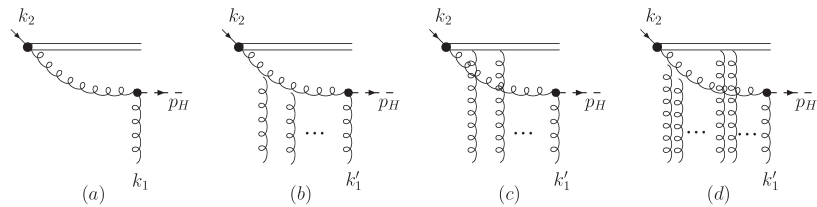
Figure 3: The generic diagrams contributing to Higgs boson production. The multiple scattering of the incoming gluon or color source inside the proton by the classical gauge field have to be re-summed to all orders. $p_{H}$ denotes the Higgs boson momentum.

The relevant diagrams for Higgs boson production are shown in Fig. 3. Before the incoming gluon from the proton combines with a gluon from the classical gauge field of the nucleus to form a Higgs boson, this gluon has initial state interactions with background gluons as it passes through the nucleus. Although they do not modify the integrated production rate, the initial state interactions change the transverse momentum distribution of the produced Higgs boson. The initial state interaction between the color source inside the proton and the classical gluon field of the nucleus should in principle also be taken into account. However, such initial state interaction, shown in Fig. 3(c) and Fig. 3(d) vanish because the ${k_{1}^{\prime}}^{+}$ poles are in the same half plane. Only Fig. 3(a) and Fig. 3(b) give non-vanishing contributions. Resuming gluon re-scattering to all orders, as illustrated in Fig. 3(b), and combining it with the contribution from Fig. 3(a), one obtains the production amplitude,

$${\cal M}=g_{\phi}(k_{2}\cdot p)\int\frac{d^{2}k_{1\perp}^{\prime}}{(2\pi)^{2}}\left(\frac{\vec{k}_{2\perp}\cdot\vec{k}_{1\perp}^{\prime}}{k_{2\perp}^{2}}\right)\langle L(k_{1\perp}-k_{1\perp}^{\prime})A^{+}(k_{1\perp}^{\prime})\rangle_{A}\phi_{p}(x_{2},k_{2\perp})$$ (16)

where the $k_{1}^{{}^{\prime}+}$ and $k_{1}^{{}^{\prime}-}$ components have been integrated out. $k_{2}=p_{H}-k_{1}$ denotes the momentum of the gluon from the proton with $p_{H}$ being the Higgs momentum. $\phi_{p}(x_{2},k_{2\perp})$ represents the probability amplitude for finding a gluon carrying a certain momentum inside the proton, with $x_{2}g(x_{2},k_{2\perp})=\phi_{p}\phi_{p}^{*}$. It is convenient to introduce the gauge potential in impact parameter space,

$$A^{+}(k_{1\perp}^{\prime})=\int dy^{-}d^{2}y_{\perp}e^{ix_{1}P^{+}y^{-}-i\vec{k}_{1\perp}^{\prime}\cdot\vec{y}_{\perp}}A^{+}(y^{-},y_{\perp})\ .$$ (17)

Replacing the exponential $e^{ix_{1}^{\prime}P^{+}y^{-}}$ by $e^{ix_{1}P^{+}y^{-}}$ in the above formula is justified in the leading logarithm approximation. Moreover, one notices that $L(k_{1\perp}-k_{1\perp}^{\prime})$ is a Wilson line which starts from $\xi^{-}$ being minus infinity and ends at the space-time point $y^{-}$,

$$L(k_{1\perp}-k_{1\perp}^{\prime})=\int d^{2}\xi_{\perp}e^{-i(\vec{k}_{1\perp}-\vec{k}_{1\perp}^{\prime})\cdot\vec{\xi}_{\perp}}{\cal P}e^{-ig\int_{-\infty^{-}}^{y^{-}}d\xi^{-}A^{+}(\xi^{-},\ \xi_{\perp})}\ .$$ (18)

We proceed by partial integration and by performing the integral over $k_{1\perp}^{\prime}$. The amplitude then can be written as,

$${\cal M} = g_{\phi}(k_{2}\cdot p)\frac{-i\vec{k}_{2\perp,i}}{k_{2\perp}^{2}}\int d^{2}y_{\perp}dy^{-}e^{ix_{1}P^{+}y^{-}-i\vec{k}_{1\perp}\cdot\vec{y}_{\perp}}$$ (19)

$$\times\langle{\cal P}e^{-ig\int_{-\infty^{-}}^{y^{-}}d\xi^{-}A^{+}(\xi^{-},y_{\perp})}F^{+i}(y^{-},y_{\perp})\rangle_{A}\phi_{p}(x_{2},k_{2\perp})\ .$$

Using the same normalization and flux factors as in the previous section, the differential cross section becomes,

$$\frac{d^{3}\sigma}{d^{2}p_{H\perp}dy}\!\!\! = \!\!\!\frac{\pi g_{\phi}^{2}}{32}\int\frac{2d^{2}k_{1\perp}}{(2\pi)^{3}}\frac{\vec{k}_{2\perp,i}\vec{k}_{2\perp,j}}{k_{2\perp}^{2}}x_{2}g(x_{2},k_{2\perp})\int d^{3}rd^{3}y$$ (20)

$$\ \ \ \ \ \times\ e^{-ix_{1}P^{+}r^{-}+i\vec{k}_{1\perp}\cdot\vec{r}_{\perp}}\langle F^{+i}(r^{-}+y^{-},r_{\perp}+y_{\perp})\,L_{r+y}^{\dagger}\,L_{y}\,F^{+j}(y^{-},y_{\perp})\rangle_{A}$$

$$= \!\!\!\sigma_{0}\int d^{2}k_{1\perp}x_{2}g(x_{2},k_{2\perp})x_{1}\left[G_{WW}(x_{1},k_{1\perp})+\left(2(\hat{k}_{1\perp}\cdot\hat{k}_{2\perp})^{2}-1\right)h^{\perp g}_{1,WW}(x_{1},k_{1\perp})\right]$$

where $\sigma_{0}=\frac{\pi g_{\phi}^{2}}{64}$ is the leading-order cross section for scalar-particle production from two gluons. Here, $y$ and $P_{H\perp}$ are rapidity and transverse momentum of the Higgs particle. In the second step of above derivation, we have made use of the normalization conditions for the average over the CGC wave function: $\langle 1\rangle_{A}=1$; and for the nuclear state $|P\rangle$ carrying momentum $P$: $\langle P^{\prime}|P\rangle=2P^{+}(2\pi)^{3}\delta(P^{+}-{P^{\prime}}^{+})\delta^{2}(P_{\perp}-P^{\prime}_{\perp})$ [27].

As observed in Ref. [14], one automatically takes into account the contribution from the linearly polarized gluon TMD in $k_{t}$ factorization. In other words, the usual unpolarized gluon distribution of the proton is the same as its linearly polarized gluon distribution in the Lipatov approximation. By noticing this fact, one finds that the differential cross section computed in TMD factorization [13, 14] completely agrees with that derived in the CGC approach. It is also worthwhile to mention that the gluon distributions entering the cross section for Higgs boson production are the WW type distributions as expected. Furthermore, in order to compare this with results from the $k_{t}$ factorization formalism, we recall that the WW type distribution $G_{WW}$ and $h^{\perp g}_{1,WW}$ become identical in the dilute region where $k_{1\perp}\gg Q_{s}$, but differ in a dense medium [8]. Therefore, in the dilute region, the differential cross section can be simplified to

$$\frac{d^{3}\sigma}{d^{2}p_{H\perp}dy}=\sigma_{0}\int d^{2}k_{1\perp}x_{2}g(x_{2},k_{2\perp})x_{1}G_{WW}(x_{1},k_{1\perp})2(\hat{k}_{1\perp}\cdot\hat{k}_{2\perp})^{2}$$ (21)

which agrees with the well known result obtained from the $k_{t}$ factorization approach [22, 21] at low Higgs transverse momentum. Thus we conclude that also for Higgs production in $pA$ the $k_{t}$ factorization formula is only valid in the dilute region. Similar conclusions have also been drawn for $\eta^{\prime}$ meson production [60] and heavy quark pair production [54] in $pA$ collisions.

4 Summary

We developed a hybrid approach for calculating particles production at central rapidity in $pA$ collisions, in which the dense target nucleus is treated in the color glass condensate model, while on the side of the dilute projectile proton the Lipatov approximation was used. As a test of the method, we first reproduced the well known result for soft gluon production in $pA$ collisions using this hybrid approach. Then, we derived the differential cross section for Higgs boson production from gluon fusion in $pA$ collisions. It turned out that the result obtained in our hybrid approach is completely equivalent to that computed in TMD factorization. In the low-density limit of $pA$ collisions, we also recover the result of the naive $k_{t}$ factorization formalism that describes Higgs boson production in $pp$ collisions adequately.

The approach developed in this article also can be applied to study the production of other color-neutral particles or heavy quark pair production in $pA$ collisions. One may expect that the CGC formalism and TMD factorization will yield the same results for these processes in a certain kinematical region. As a consequence, the Weizsäcker-Williams and dipole type linearly polarized gluon distributions could be extracted by measuring azimuthal asymmetries in these processes. We will address these issues in a forthcoming paper [61].

Acknowledgments: This work has been supported by BMBF (OR 06RY9191).

References

- [1] D. Boer, M. Diehl, R. Milner, R. Venugopalan, W. Vogelsang, D. Kaplan, H. Montgomery and S. Vigdor et al., arXiv:1108.1713 [nucl-th].
- [2] P. J. Mulders and J. Rodrigues, Phys. Rev. D 63, 094021 (2001) [arXiv:hep-ph/0009343].
- [3] M. Anselmino, M. Boglione, U. D’Alesio, E. Leader, S. Melis and F. Murgia, Phys. Rev. D 73, 014020 (2006) [hep-ph/0509035].
- [4] S. Meissner, A. Metz and K. Goeke, Phys. Rev. D 76, 034002 (2007) [arXiv:hep-ph/0703176].
- [5] D. Boer and P. J. Mulders, Phys. Rev. D 57, 5780 (1998) [arXiv:hep-ph/9711485].
- [6] S. J. Brodsky, D. S. Hwang and I. Schmidt, Phys. Lett. B 530, 99 (2002) [arXiv:hep-ph/0201296].
- [7] J. C. Collins, Phys. Lett. B 536, 43 (2002) [arXiv:hep-ph/0204004].
- [8] A. Metz, J. Zhou, Phys. Rev. D84, 051503 (2011). [arXiv:1105.1991 [hep-ph]].
- [9] D. Boer, P. J. Mulders and C. Pisano, Phys. Rev. D 80, 094017 (2009) [arXiv:0909.4652 [hep-ph]].
- [10] D. Boer, S. J. Brodsky, P. J. Mulders and C. Pisano, Phys. Rev. Lett. 106, 132001 (2011) [arXiv:1011.4225 [hep-ph]].
- [11] J. -W. Qiu, M. Schlegel and W. Vogelsang, Phys. Rev. Lett. 107, 062001 (2011) [arXiv:1103.3861 [hep-ph]].
- [12] M. Anselmino et al., Eur. Phys. J. A 47, 35 (2011) [arXiv:1101.4199 [hep-ex]].
- [13] D. Boer, W. J. den Dunnen, C. Pisano, M. Schlegel and W. Vogelsang, Phys. Rev. Lett. 108, 032002 (2012) [arXiv:1109.1444 [hep-ph]].
- [14] P. Sun, B. -W. Xiao, F. Yuan, Phys. Rev. D84, 094005 (2011). [arXiv:1109.1354 [hep-ph]].
- [15] A. V. Manohar and W. J. Waalewijn, arXiv:1202.3794 [hep-ph] and references therein.
- [16] M. Garcia-Echevarria, A. Idilbi and I. Scimemi, arXiv:1111.4996 [hep-ph] and references therein.
- [17] S. Catani, M. Grazzini, Nucl. Phys. B845, 297-323 (2011). [arXiv:1011.3918 [hep-ph]].
- [18] S. Mantry, F. Petriello, Phys. Rev. D81, 093007 (2010). [arXiv:0911.4135 [hep-ph]]; and references therein.
- [19] P. M. Nadolsky, C. Balazs, E. L. Berger, C. -P. Yuan, Phys. Rev. D76, 013008 (2007). [hep-ph/0702003 [HEP-PH]].
- [20] J. Collins, (Cambridge monographs on particle physics, nuclear physics and cosmology. 32)
- [21] F. Hautmann, Phys. Lett. B535, 159-162 (2002). [hep-ph/0203140].
- [22] A. V. Lipatov, N. P. Zotov, Eur. Phys. J. C44, 559-566 (2005). [hep-ph/0501172].
- [23] R. S. Pasechnik, O. V. Teryaev and A. Szczurek, Eur. Phys. J. C 47, 429 (2006) [hep-ph/0603258].
- [24] Y. V. Kovchegov, Phys. Rev. D 54, 5463 (1996) [arXiv:hep-ph/9605446].
- [25] J. Jalilian-Marian, A. Kovner, L. D. McLerran and H. Weigert, Phys. Rev. D 55, 5414 (1997) [arXiv:hep-ph/9606337].
- [26] F. Dominguez, B. W. Xiao and F. Yuan, Phys. Rev. Lett. 106, 022301 (2011) [arXiv:1009.2141 [hep-ph]].
- [27] F. Dominguez, C. Marquet, B. W. Xiao and F. Yuan, Phys. Rev. D 83, 105005 (2011) [arXiv:1101.0715 [hep-ph]].
- [28] L. D. McLerran and R. Venugopalan, Phys. Rev. D 49, 2233 (1994) [arXiv:hep-ph/9309289]; Phys. Rev. D 49, 3352 (1994) [arXiv:hep-ph/9311205].
- [29] A. H. Mueller, arXiv:hep-ph/0111244.
- [30] E. Iancu, A. Leonidov and L. McLerran, arXiv:hep-ph/0202270.
- [31] F. Gelis, E. Iancu, J. Jalilian-Marian and R. Venugopalan, Ann. Rev. Nucl. Part. Sci. 60, 463 (2010) [arXiv:1002.0333 [hep-ph]].
- [32] E. A. Kuraev, L. N. Lipatov, V. S. Fadin, Sov. Phys. JETP 45, 199-204 (1977).
- [33] L. V. Gribov, E. M. Levin, M. G. Ryskin, Phys. Rept. 100, 1-150 (1983).
- [34] S. Catani, M. Ciafaloni, F. Hautmann, Nucl. Phys. B366, 135-188 (1991).
- [35] J. C. Collins, R. K. Ellis, Nucl. Phys. B360, 3-30 (1991).
- [36] A. Dumitru, J. Jalilian-Marian, Phys. Rev. D81, 094015 (2010). [arXiv:1001.4820 [hep-ph]]. A. Dumitru, J. Jalilian-Marian, Phys. Rev. D82, 074023 (2010) [arXiv:1008.0480 [hep-ph]].
- [37] F. Dominguez, A. H. Mueller, S. Munier, B. -W. Xiao, Phys. Lett. B705, 106-111 (2011). [arXiv:1108.1752 [hep-ph]].
- [38] F. Dominguez, J. -W. Qiu, B. -W. Xiao, F. Yuan, [arXiv:1109.6293 [hep-ph]].
- [39] A. Dumitru, J. Jalilian-Marian, T. Lappi, B. Schenke, R. Venugopalan, [arXiv:1108.4764 [hep-ph]].
- [40] E. Iancu, D. N. Triantafyllopoulos, [arXiv:1109.0302 [hep-ph]].
- [41] J. Jalilian-Marian, [arXiv:1111.3936 [hep-ph]].
- [42] E. Iancu and D. N. Triantafyllopoulos, JHEP 1204, 025 (2012) [arXiv:1112.1104 [hep-ph]].
- [43] J. Jalilian-Marian, A. Kovner, A. Leonidov, H. Weigert, Phys. Rev. D59, 014014 (1999). [hep-ph/9706377]. J. Jalilian-Marian, A. Kovner, A. Leonidov, H. Weigert, Nucl. Phys. B504, 415-431 (1997). [hep-ph/9701284]. E. Iancu, A. Leonidov, L. D. McLerran, Nucl. Phys. A692, 583-645 (2001). [hep-ph/0011241]. E. Ferreiro, E. Iancu, A. Leonidov, L. McLerran, Nucl. Phys. A703, 489-538 (2002). [hep-ph/0109115].
- [44] B. Z. Kopeliovich, A. V. Tarasov, A. Schäfer, Phys. Rev. C59, 1609-1619 (1999). [hep-ph/9808378].
- [45] Y. V. Kovchegov, A. H. Mueller, Nucl. Phys. B529, 451-479 (1998). [hep-ph/9802440].
- [46] D. Kharzeev, Y. V. Kovchegov, K. Tuchin, Phys. Rev. D68, 094013 (2003). [hep-ph/0307037].
- [47] A. Dumitru, L. D. McLerran, Nucl. Phys. A700, 492-508 (2002). [hep-ph/0105268].
- [48] J. P. Blaizot, F. Gelis, R. Venugopalan, Nucl. Phys. A743, 13-56 (2004). [hep-ph/0402256].
- [49] F. Gelis, Y. Mehtar-Tani, Phys. Rev. D73, 034019 (2006). [hep-ph/0512079].
- [50] E. Avsar, arXiv:1203.1916 [hep-ph].
- [51] I. Balitsky, Nucl. Phys. B463, 99-160 (1996). [hep-ph/9509348].
- [52] L. D. McLerran, R. Venugopalan, Phys. Rev. D59, 094002 (1999). [hep-ph/9809427].
- [53] F. Gelis, A. Peshier, Nucl. Phys. A697, 879-901 (2002). [hep-ph/0107142].
- [54] J. P. Blaizot, F. Gelis, R. Venugopalan, Nucl. Phys. A743, 57-91 (2004). [hep-ph/0402257].
- [55] K. Fukushima, Y. Hidaka, JHEP 0706, 040 (2007). [arXiv:0704.2806 [hep-ph]].
- [56] M. Braun, Eur. Phys. J. C16, 337-347 (2000). [hep-ph/0001268].
- [57] M. A. Braun, Phys. Lett. B483, 105-114 (2000). [hep-ph/0003003].
- [58] J. C. Collins and D. E. Soper, Nucl. Phys. B 194, 445 (1982).
- [59] X. -d. Ji, J. -P. Ma and F. Yuan, JHEP 0507, 020 (2005) [hep-ph/0503015].
- [60] F. Fillion-Gourdeau, S. Jeon, Phys. Rev. C79, 025204 (2009). [arXiv:0808.2154 [hep-ph]].
- [61] E. Akcakaya, A. Metz, A. Schäfer, J. Zhou, in preparation.