A Generic Hopf Algebra for Quantum Statistical Mechanics

Abstract

In this note we present a Hopf algebra description of a bosonic quantum model, using the elementary combinatorial elements of Bell and Stirling numbers. Our objective in doing this is the following. Recent studies have revealed that perturbative Quantum Field Theory (pQFT) displays an astonishing interplay between analysis (Riemann Zeta functions), topology (Knot theory), combinatorial graph theory (Feynman Diagrams) and algebra (Hopf structure). Since pQFT is an inherently complicated study, thus far not exactly solvable and replete with divergences, the essential simplicity of the relationships between these areas can be somewhat obscured. The intention here is to display some of pevious-mentioned structures in the context of a simple bosonic quantum theory; i.e. a quantum theory of non-commuting operators which do not depend on spacetime. The combinatorial properties of these boson creation and annihilation operators, which is our chosen example, may be described by graphs, analogous to the Feynman diagrams of pQFT, which we show possess a Hopf algebra structure. Our approach is based on the quantum canonical partition function for a boson gas.

1 Bell and Stirling numbers

A basic combinatorial construct is the Bell number, $B(n)$. This gives the number of ways in which $n$ distinct objects may be distributed among $n$ identical containers, some of which may remain empty. The first few values of $B(n)$ are

$$B(n)=1,\,1,\,2,\,5,\,15,\,52,\,203,\,\ldots,\quad n=0,\,1,\,2,\,\ldots\,.$$

These values grow rapidly, but less so than $n!$

Related to the Bell numbers are the Stirling numbers (of the second kind) $S(n,k)$, which are defined as the number of ways of putting $n$ different objects into $k$ identical containers, leaving none empty. From the definition we have $B(n)=\sum_{k=1}^{n}S(n,k)$.

A compact way of defining a combinatorial sequence is by means of a generating function. For the Bell numbers, the exponential generating function is given by

$$\sum_{n=0}^{\infty}{B(n)}\,\frac{x^{n}}{n!}=\exp(e^{x}-1)$$ (1)

A slight generalization of the exponential generating function for the Bell numbers is given by that defining the Bell polynomials $B_{n}(y)$:

$$\exp\left(y\bigl{(}e^{x}-1\bigr{)}\right)=\sum_{n=0}^{\infty}B_{n}(y)\,\frac{x^{n}}{n!}$$ (2)

Note that

$$B_{n}(y)=\sum_{k=0}^{n}{S(n,k){y^{k}}}.$$ (3)

1.1 Normal order

Although somewhat unfamiliar to physicists, the Bell and Stirling numbers are fundamental in quantum theory. This is because they arise naturally in the normal ordering problem of bosonic operators. By the normal ordering operation ${\mathcal{N}}f(a,a^{\dagger})$ we mean reorder the boson operators in $f(a,a^{\dagger})$ so that all annihilation operators are on the right. For canonical boson creation and annihilation operators $\{a^{\dagger},a\}$ satisfying $[a,a^{\dagger}]=1$, the Stirling numbers of the second kind $S(n,k)$ intervene through [1, 2]

$${\mathcal{N}}(a^{\dagger}a)^{n}=\sum_{k=1}^{n}S(n,k)(a^{\dagger})^{k}a^{k}\,.$$ (4)

The corresponding Bell numbers $B(n)=\sum_{k=1}^{n}S(n,k)$ are simply the expectation values

$$B(n)=\langle z|(a^{\dagger}a)^{n}|z\rangle_{z=1}$$ (5)

taken in the coherent state defined by

$$a|z\rangle=z|z\rangle$$ (6)

for $z=1$. In fact, for physicists, these equations may be taken as the definitions of the Stirling and Bell numbers.

1.2 Graphs

We now give a graphical representation of the Bell numbers, based on work of Brody, Bender and Meister [3, 4], which we have extended in [5]. Consider labelled lines which emanate from a white dot, the origin, and finish on a black dot, the vertex. We shall allow only one line from each white dot but impose no limit on the number of lines ending on a black dot. Clearly this simulates the definition of $S(n,k)$ and $B(n)$, with the white dots playing the role of the distinguishable objects, whence the lines are labelled, and the black dots that of the indistinguishable containers. The identification of the graphs for 1, 2 and 3 lines is given in Figure 1 below.

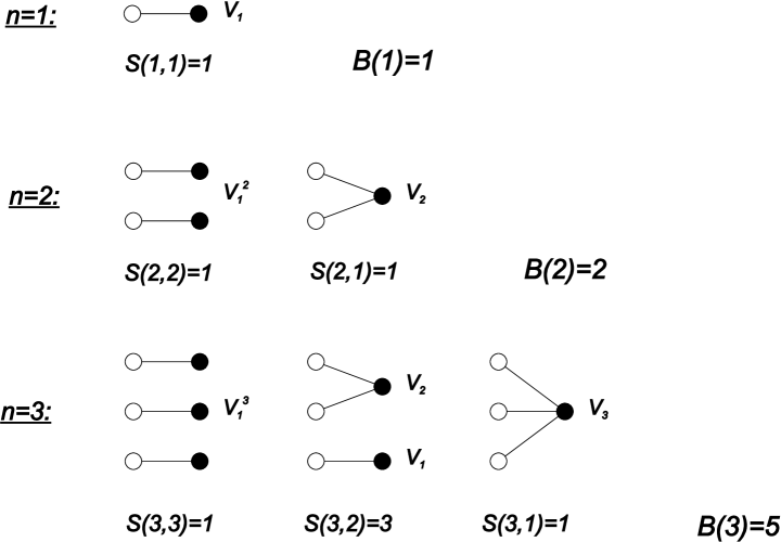
Figure 1: Graphs for $B(n)$, $n=1$, 2, 3.

We have concentrated on the Bell number sequence and its associated graphs since, as we shall show, there is a sense in which this sequence of graphs is generic in the evaluation of the Quantum Partition Function. By this we mean the following: We first show below that the Bell number sequence arises from the Partition Function of a non-interacting boson model. Then, when interactions are present these may be incorporated by the use of suitable strengths associated with the vertices of the graphs. That is, we can represent the combinatorial sequence of an interacting model by the same sequence of graphs as in Figure 1, with suitable vertex multipliers (denoted by the $V$ terms in the same figure).

2 Partition Function Integrand

We now show the relation of the preceding considerations to the computation of the Canonical partition Function $Z$ in Quantum Statistical Mechanics, and introduce the Partition Function Integrand, which is directly related to the combinatorial Bell numbers.

2.1 Free boson gas and Bell polynomials

The canonical partition function associated with the hamiltonian $H$ is given by

$$Z={\rm Tr}\exp(-\beta H)\,.$$ (7)

We take the elementary case of the hamiltonian for the single–mode free boson gas $H=\epsilon a^{\dagger}a$ (ignoring an additive constant), $\epsilon>0$. The usual computation of the partition function, exploiting the completeness property $\sum_{n=0}^{\infty}|n\rangle\langle n|=I$, is immediate:

$$Z = {\rm Tr}\exp(-\beta\epsilon a^{\dagger}a)$$ (8)

$$= \sum_{n=0}^{\infty}{\langle n|e^{-\beta\epsilon\hat{n}}|n\rangle}$$ (9)

$$= \sum_{n=0}^{\infty}{e^{-\beta\epsilon n}}$$ (10)

$$= \left(1-e^{-\beta\epsilon}\right)^{-1}\,.$$ (11)

However, we may use any complete set to perform the trace. We choose coherent states as defined in Eq.(6) above, which are explicitly given by

$$|z\rangle=e^{-|z|^{2}/2}\sum_{n}({{z^{n}}{/n!}){a^{\dagger}}^{n}}|0\rangle.$$ (12)

For these states the completeness or resolution of unity property is

$$\frac{1}{\pi}\int d^{2}z|z\rangle\langle z|=I\equiv\int d\mu(z)|z\rangle\langle z|.$$ (13)

The appropriate trace calculation is

$$Z = \frac{1}{\pi}\int d^{2}z\langle z|\exp\bigl{(}-\beta\epsilon a^{\dagger}a\bigr{)}|z\rangle=$$ (14)

$$= \frac{1}{\pi}\int d^{2}z\langle z|:\exp\bigl{(}a^{\dagger}a(e^{-\beta\epsilon}-1)\bigr{)}:|z\rangle\,,$$ (15)

where we have used the following well-known relation [6, 7] for the forgetful normal ordering operator $:\!f(a,a^{\dagger})\!:$ which means “normally order the creation and annihilation operators in $f$ forgetting the commutation relation $[a,a^{\dagger}]=1$”:

$${\mathcal{N}}exp(xa^{\dagger}a)=:\exp\bigl{(}a^{\dagger}a(e^{x}-1)\bigr{)}:.$$ (16)

We therefore obtain, integrating over the angle variable $\theta$ and the radial variable $r=|z|$,

$$Z=\frac{1}{\pi}\int_{0}^{2\pi}d\theta\int_{0}^{\infty}r\,dr\exp\left(r^{2}\bigl{(}e^{-\beta\epsilon}-1\bigr{)}\right)\,,$$ (17)

which gives us $Z=\bigl{(}1-e^{-\beta\epsilon}\bigr{)}^{-1}$ as before.

We rewrite the above equation to show the connection with our previously–defined combinatorial numbers. Writing $y=r^{2}$ and $x=-\beta\epsilon$, Eq.(17) becomes

$$Z=\int\limits_{0}^{\infty}dy\exp\bigl{(}y(e^{x}-1)\bigr{)}\,.$$ (18)

This is an integral over the classical exponential generating function for the Bell polynomials as given in Eq.(2). This leads to the combinatorial form for the partition function

$$Z=\int_{0}^{\infty}dy\sum_{n=0}^{\infty}B_{n}(y)\,\frac{x^{n}}{n!}\,.$$ (19)

Although Eq.(19) is remarkably simple in form, it is often by no means a straightforward matter to evaluate the analogous integral for other than the free boson system considered here. Further, it is also clear that we may not interchange the integral and the summation, as each individual $y$ integral diverges. We shall therefore concentrate in what follows on the partition function integrand (PFI) $F(z)=\langle z|\exp(-\beta H)|z\rangle$, whence $Z=\int F(z)\,d\mu(z)$, to give a graphical description of a perturbation approach. The function $F$ maps coherent states $|z\rangle$ to (real) numbers, and is therefore a functional on the coherent states..

2.2 General partition functions

We now apply this graphical approach to the general partition function in second quantized form. With the usual definition for the partition function Eq.(7). In general the hamiltonian is given by $H=\epsilon w(a,a^{\dagger})$, where $\epsilon$ is the energy scale, and $w$ is a string (= sum of products of positive powers) of boson creation and annihilation operators. The partition function integrand $F$ for which we seek to give a graphical expansion, is

$$Z(x)=\int{F(x,z)\,d\mu(z)}\,,$$ (20)

where

$$F(x,z) = \langle z|\exp(xw)|z\rangle=\hskip 56.9055pt(x=-\beta\epsilon)$$ (21)

$$= \sum_{n=0}^{\infty}\langle z|w^{n}|z\rangle\,\frac{x^{n}}{n!}$$

$$= \sum_{n=0}^{\infty}W_{n}(z)\,\frac{x^{n}}{n!}$$

$$= \exp\biggl{(}\;\sum_{n=1}^{\infty}V_{n}(z)\,\frac{x^{n}}{n!}\biggr{)},$$

with obvious definitions of $W_{n}$ and $V_{n}$. The sequences $\left\{W_{n}\right\}$ and $\left\{V_{n}\right\}$ may each be recursively obtained from the other [8]. This relates the sequence of multipliers $\{V_{n}\}$ of Figure 1 to the hamiltonian of Eq.(7). The lower limit $1$ in the $V_{n}$ summation is a consequence of the normalization of the coherent state $|z\rangle$.

At this point the analogue of this model to perturbative quantum field theory becomes more transparent. For example, to calculate the partition Function $Z(x)$, we must integrate over the Partition Function Integrand $F(x,z)$. Here, the integration over the coherent state parameter $z$ plays the role of the space-time integration of Quantum Field Theory. As noted above with reference to Eq.(19) for the non-interacting case, and as in pQFT, term-by-term integration, corresponding to fallaciously interchanging the summation and integration actions, results in infinities at each term, as can be directly verified even in the non-interacting case. Thus even here an elementary form of renormalization is necessary, if we have to resort to term-wise integration.

Considerations such as these have led many authors, as noted in reference [10], to consider a global, algebraic approach to pQFT; and this we now do in the context of our simple model.

3 Hopf Algebra structure

To describe the Hopf Algebra structure of our model, which we shall refer to as BELL below, we first introduce a basic Hopf Algebra, which we call POLY, generated by a single parameter $x$. This is essentially a standard one-variable polynomial algebra on which we impose the Hopf operation of co-product, co-unit and antipode, as a useful pedagogical device for describing their properties. The Hopf structure associated with our model described above is simply a multi-variable extension of POLY.

3.1 The Hopf Algebra POLY

POLY consists of polynomials in $x$ (say, over the real field $\mathcal{R}$, for example).The standard algebra structure of addition and associative multiplication is obtained in the usual way, by polynomial addition and multiplication. The additional Hopf operations are:

1. The coproduct $\Delta:{\bf POLY}\longrightarrow{\bf POLY}\times{\bf POLY}$ is defined by

   $$\Delta(e) = e\times e\;\;\;\;({\rm unit}\;\;e)$$

   $$\Delta(x) = x\times e+e\times x\;\;\;\;({\rm generator}\;\;x)$$

   $$\Delta(AB) = \Delta(A)\Delta(B)\;\;\;{\rm otherwise}$$

   so that $\Delta$ is an algebra homomorphism.

2. The co-unit $\epsilon$ satisfies $\epsilon(e)=1$ otherwise $\epsilon(A)=0$.

3. The antipode ${\mathcal{S}}:{\bf POLY}\longrightarrow{\bf POLY}$ satisfies ${\mathcal{S}}(e)=e$; on the generator $x$, ${\mathcal{S}}(x)=-x$. It is an anti-homomorphism, i.e. ${\mathcal{S}}(AB)={\mathcal{S}}(B){\mathcal{S}}(A)$.

It may be shown that the foregoing structure ${\bf POLY}$ satisfies the axioms of a commutative, co-commutative Hopf algebra.

3.2 BELL

We now briefly describe the Hopf algebra ${\bf BELL}$ which is appropriate for the diagram structure introduced in this note, defined by the diagrams of Figure 1.

1. Each distinct diagram is an individual basis element of ${\bf BELL}$; thus the dimension is infinite. (Visualise each diagram in a “box”.) The sum of two diagrams is simply the two boxes containing the diagrams. Scalar multiples are formal; for example, they may be provided by the $V$ coefficients.

2. The identity element $e$ is the empty diagram (an empty box).

3. Multiplication is the juxtaposition of two diagrams within the same “box”. ${\bf BELL}$ is generated by the connected diagrams; this is a consequence of the Connected Graph Theorem [9]. Since we have not here specified an order for the juxtaposition, multiplication is commutative.

4. The coproduct $\Delta:{\bf BELL}\longrightarrow{\bf BELL}\times{\bf BELL}$ is defined by

   $$\Delta(e) = e\times e\;\;\;\;({\rm unit}\;\;e)$$

   $$\Delta(y) = y\times e+e\times y\;\;\;\;({\rm generator}\;\;y)$$

   $$\Delta(AB) = \Delta(A)\Delta(B)\;\;\;{\rm otherwise}$$

   so that $\Delta$ is an algebra homomorphism.

5. The co-unit $\epsilon$ satisfies $\epsilon(e)=1$ otherwise $\epsilon(A)=0$.

6. The antipode ${\mathcal{S}}:{\bf BELL}\longrightarrow{\bf BELL}$ satisfies ${\mathcal{S}}(e)=e$; on a generator $x$, ${\mathcal{S}}(y)=-y$. It is an anti-homomorphism, i.e. ${\mathcal{S}}(AB)={\mathcal{S}}(B){\mathcal{S}}(A)$.

3.3 BELL as an extension of POLY

It may be seen that ${\bf BELL}$ is a multivariable version of ${\bf POLY}$. To show this, we code the diagrams by letters. We use an infinite alphabet $Y=\{y_{1},y_{2},y_{3}\cdots\}=\{y_{k}\}_{k\geq 1}$ and code each connected diagram with one black spot and $k$ white spots with the letter $y_{k}$. An unconnected diagram will be coded by the product of its letters.
In this way, the diagrams of Figure 1 are coded as follows:

• first line : $y_{1}$

• second line : $y_{1}^{2}$ and $y_{2}$

• third line : $y_{1}^{3}$ and $y_{1}y_{2}$ and $y_{3}$ .

Thus one sees that each diagram of weight $n$ with $k$ connected components is coded bijectively by a monomial of weight $n$ (the weight of a monomial $y_{i_{1}}y_{i_{2}}\cdots y_{i_{r}}$ is just the sum of the indices $\sum_{j=1}^{r}i_{j}$) and $k$ letters. The algebra ${\bf BELL}$ is coded by commutative polynomials in the infinite alphabet $Y$; that is, the coding is an isomorphism ${\bf BELL}\rightarrow{\mathcal{R}}[Y]$. As an aside, one may note that the basis elements of ${\bf BELL}$ are sometimes referred to as forests. As above, it may be shown that the foregoing structure ${\bf BELL}$ satisfies the axioms of a commutative, co-commutative Hopf algebra.

4 Discussion

The objective of this note was to introduce a very simple Hopf structure associated with standard bosonic creation and annihilation operators, in the context of the evaluation of the canonical partition function of quantum statistical mechanics. We did this via a diagrammatic description applied to a non-interacting boson gas, but implied that the algebraic description was general enough to include interactions as scalar coefficients. The inspiration for this task arose from considering recent work on perturbative quantum field theory (pQFT)[10], where it has been shown that a Hopf description is available for this far more complicated system. It is instructive to consider a much more straightforward system, such as the one treated here, where the operators do not depend on space or time. Nevertheless, we have shown that even such a basic system does exhibit some of the features of the more complicated case, in particular the structure of a Hopf algebra, which we called ${\bf BELL}$. This may be thought of as a simple solvable model in its own right.

However, one may also ask wherein does this simple structure sit within the full pQFT structure? The strategy which we adopt, and which we describe in further work, is to generalize the algebraic structure, and thereby produce Hopf algebras of sufficient complexity to emulate those associated with pQFT. In subsequent work we show that by suitable deformation of the Hopf algebra described here we obtain structures related to those arising from more realistic models, such as those associated with pQFT.

Acknowlegements

The authors wish to acknowledge support from the Agence Nationale de la Recherche (Paris, France) under Program No. ANR-08-BLAN-0243-2 and from PAN/CNRS Project PICS No.4339(2008-2010) as well as the Polish Ministry of Science and Higher Education Grant No.202 10732/2832.

References

References

- [1] J. Katriel: Lett. Nuovo Cimento 10 (1974) 565.
- [2] J. Katriel: Phys. Lett. A. 273 (2000) 159.
- [3] Bender CM, Brody DC and Meister BK 1999 Quantum field theory of partitions, J.Math. Phys. 40 3239
- [4] Bender CM, Brody DC and Meister BK 2000 Combinatorics and field theory, Twistor Newsletter 45 36
- [5] Blasiak P, Penson KA , Solomon AI, Horzela A and Duchamp GEH, 2005 J.Math.Phys. 46, 052110 ( and arXiv:quant-ph/0405103
- [6] Klauder JR and Sudarshan ECG 1968 Fundamentals of Quantum Optics (Benjamin, New York)
- [7] Louisell WH 1990 Quantum Statistical Properties of Radiation (J. Wiley, New York)
- [8] Pourahmadi 1984 Amer. Math. Monthly 91, 303
- [9] Ford GW and Uhlenbeck GE 1956 Proc. Nat. Acad. 42, 122
- [10] A readable account may be found in Dirk Kreimer 2000 Knots and Feynman Diagrams Cambridge Lecture Notes in Physics, (Cambridge University Press)