Can bipartite classical information resources be activated?

Abstract

Non-additivity is one of the distinctive traits of Quantum Information Theory: the combined use of quantum objects may be more advantageous than the sum of their individual uses. Non-additivity effects have been proven, for example, for quantum channel capacities, entanglement distillation or state estimation. In this work, we consider whether non-additivity effects can be found in Classical Information Theory. We work in the secret-key agreement scenario in which two honest parties, having access to correlated classical data that are also correlated to an eavesdropper, aim at distilling a secret key. Exploiting the analogies between the entanglement and the secret-key agreement scenario, we provide some evidence that the secret-key rate may be a non-additive quantity. In particular, we show that correlations with conjectured bound information become secret-key distillable when combined. Our results constitute a new instance of the subtle relation between the entanglement and secret-key agreement scenario.

Introduction

Classical communication systems are governed by classical information theory, a vast discipline whose birth coincides with a seminal paper of Claude Shannon [1]. Among his contributions, Shannon introduced the concept of channel capacity, which quantifies the maximum communication rate that can be achieved over a classical channel. One key feature of the channel capacity is its additivity: the total capacity of several channels used in parallel is simply given by the sum of their individual capacities. This fact implies thus that the channel capacity completely specifies channel’s ability to convey classical information.

Moving to the quantum domain, the quantum channel capacity captures the ability of a quantum channel to transmit quantum information. Smith and Yard [2] proved recently that the quantum capacity is not additive. In particular, they provide examples of two channels with zero quantum capacity that define a channel with strictly positive quantum capacity when combined. This intriguing quantum effect is known as activation and can generally be understood as follows: the combined use of quantum objects can be more advantageous than the sum of their individual uses. In the last years, an intense effort has been devoted to the study of non-additivity effects in Quantum Information Theory. Classical and private communication capacity of quantum channels were later shown not to be additive in Refs [3, 4]. Nowadays, non-additivity is considered to be one of the distinctive traits of Quantum Information Theory.

Before the results by Smith and Yard, however, non-additivity effects had also been observed in Entanglement Theory in the context of entanglement distillation. There, one is interested in the problem of whether pure-state entanglement –pure entanglement in what follows– can be extracted from a given state shared by several observers using local operations and classical communication (LOCC). In Ref. [5], the authors provide examples of multipartite states that (i) are non-distillable (bound) when considered separately but (ii) define a distillable state when taken together. Moving to the case of two parties, and leaving aside activation-like results as those of [6], it remains unproven whether entangled states can be activated. There is however some evidence of the existence of pairs of bound (non-distillable) entangled states that give a distillable state when combined [7, 8].

In this work we are interested in the question of whether non-additivity effects can be observed in Classical Information Theory. As mentioned, classical channel capacities are known to be additive. Therefore, we move our considerations to distillation scenarios. In particular, we focus on the classical secret-key agreement scenario in which two honest parties, having access to correlated random variables, also correlated with an adversary, aim at establishing a secret key by local operations and public communication (LOPC). While the activation of classical resources has been shown in a multipartite key-agreement scenario in [9, 10], here we consider the more natural case of two honest parties. In our study, we exploit the analogies between the secret-key agreement and entanglement scenario noted in [11]. Based on the results of [8], we provide evidence that activation effects may be possible in the completely classical bipartite key-agrement scenario. Our findings, therefore, suggest that the classical secret-key rate is non-additive.

This article is structured as follows: Section 1 contains a brief introduction to the entanglement and the secret-key agreement scenario. After pointing out the analogies between the two scenarios, our main results are derived in section 2. Section 3 concludes with a discussion of how our findings are related to other results and conjectures in the field.

1 Entanglement vs secret correlations

The aim of this section is to introduce the entanglement and secret-key agreement scenario. As first noted in [12], there are several analogies between these two scenarios despite the fact that they involve objects of different nature, namely entangled quantum states vs classical joint probability distributions. These analogies play a key role in the derivation of our results in the next section.

1.1 Entanglement scenario

A maximally entangled state of two qubits represents the most representative example of a bipartite entangled state and is an essential ingredient in many applications of quantum information theory [13]. It is defined as:

$$|\phi\rangle=\frac{1}{\sqrt{2}}\left(\big{|}00\big{\rangle}+\big{|}11\big{\rangle}\right)_{AB}$$ (1)

The relevance of this state for communication purposes is due essentially to two main facts: first, for each projective measurement by one of the observers, there exists another measurement by the other observer giving perfectly correlated results. Second, being a pure state, no third party can be correlated with it. State (1) represents the basic unit of entanglement and is also known as ebit, for entangled bit. This is because an asymptotically large number of copies of an arbitrary pure entangled state can be converted into another asymptotically large number of ebits in a reversible way [14].

In any realistic situation, quantum states are affected by noise. In the case of a composite system shared by two observers, Alice and Bob (also $A$ and $B$), the ideal pure entangled states is mapped into a mixed state $\rho_{AB}$. Any noise can be modeled as interaction with an environment, $E$, as any state can be seen as the trace of a pure state on a sufficiently large environment. In the bipartite case considered here one has $\rho_{AB}=\mathrm{tr}_{E}|\psi_{ABE}\rangle\!\langle\psi_{ABE}|$. Of course, the interaction with the environment deteriorates the entanglement present in the state. Thus, given a generic quantum state $\rho_{AB}$, or equivalently the whole tripartite state $|\psi_{ABE}\rangle$, quantifying the entanglement between $A$ and $B$ is a fundamental question. Two quantifiers play a crucial role because of their operational meaning: the entanglement cost and the entanglement of distillation. Both quantities are defined in the asymptotic scenario consisting of an asymptotically large number of identical copies of the state. The entanglement cost [15], denoted by $E_{c}$, quantifies the number of ebits per copy needed for the formation of the given quantum state by LOCC. The entanglement of distillation [16], denoted by $E_{D}$, indicates the amount of ebits per copy that can be obtained from it by LOCC. For a state $\rho_{AB}$, $E_{c}(\rho_{AB})>0$ implies that the state is entangled, while $E_{D}(\rho_{AB})>0$ indicates that some pure entanglement can be extracted from it. Clearly, it holds that $E_{c}\geq E_{D}$, as one cannot extract from a state more entanglement than needed for its preparation. Interestingly, there are states that display an intriguing form of irreversibility: despite having a positive entanglement cost ($E_{c}>0$), they are non-distillable ($E_{D}=0$). These states are called bound entangled [17]. Consequently, the whole set of entangled states is composed of distillable, or free entangled states, and bound entangled states.

Detecting whether a given state is non-distillable is in principle a very hard question, as one has to prove that no LOCC protocol acting on an arbitrary number of copies of the state is able to extract any pure entanglement. However, a very useful result derived in [17] shows that a quantum state that remains Positive under Partial Transposition [18] (PPT) is non-distillable. Whether Non-Positivity of the Partial Transposition, or Negative Partial Transposition (NPT), is sufficient for entanglement distillability is probably the main open question at the moment in Entanglement Theory. Evidence [19, 20] has been given for the existence of NPT states that are bound entangled (see however [21]). Note that the existence of these states would imply that the set of non-distillable states is not convex and that entanglement of distillation is non-additive [7]. A necessary and sufficient condition for the distillability of a quantum state is provided by the following

Theorem 1.

A state $\rho$ acting on ${\cal H}={\cal H}_{A}\otimes{\cal H}_{B}$ is distillable if and only if there exist a finite integer number $n\geq 1$ and two dimensional projectors $P:{\cal H}^{\otimes n}_{A}\rightarrow\mathbb{C}^{2}$ and $Q:{\cal H}^{\otimes n}_{B}\rightarrow\mathbb{C}^{2}$ such that the state

$$\rho^{\prime}=(P\otimes Q)\rho^{\otimes n}(P\otimes Q)^{\dagger}$$ (2)

is entangled.

Actually, since the resulting state acts on $\mathbb{C}^{2}\otimes\mathbb{C}^{2}$, this is equivalent to demand that $\rho^{\prime}$ is NPT, as this condition is necessary and sufficient for entanglement in the two-qubit case [22]. Furthermore, it is worth mentioning here that, if such a projector exists for some number $k$ of copies, the state is said to be $k-distillable$.

1.2 Secret-key agreement scenario

The main scope of this section is to introduce the secret-key agreement scenario. This scenario consists of two honest parties, again Alice and Bob, who have access to correlated information, described by two random variables $X$ and $Y$. These variables are also correlated to a third random variable $Z$ that belongs to an adversarial party, the eavesdropper Eve, denoted by $E$. All the correlations among the three parties are described by the probability distribution $P(XYZ)$. The honest parties aim at mapping the initial correlations into a secret key by LOPC, which is the natural set of operations between the honest parties.

Similar questions as above can be addressed in this completely classical scenario. The classical equivalent of a maximally entangled state is a secret bit. $A$ and $B$ share perfect secret bits whenever $P(XYZ)$ is such that the eavesdropper is factored out, $P(XY)\times P(Z)$, and their variables can take two possible values, $X,Y=0,1$, that are perfectly correlated and random, $P(X=Y=0)=P(X=Y=1)=1/2$. Similarly as above, given some initial correlations, the goal is to quantify its secrecy content. The classical analog of $E_{c}$ is the information of formation, denoted by $I_{f}$ [23]. It is said that the probability distribution $P(XYZ)$ contains secret correlations (or secret bits) whenever $I_{f}(P(XYZ))>0$. For distillation, the natural classical analog is the secret-key rate [24], denoted by $S(X:Y\|Z)$, which quantifies the number of secret bits that can be distilled from given correlations by LOPC. Due to the difficulty of computing the previous quantities, it is useful to establish bounds on them. The intrinsic information [24], $I(X;Y\downarrow Z)$, provides a lower bound to the information of formation [23] and an upper bound to the secret-key rate [24]:

$$S(X;Y\|Z)\leq I(X;Y\downarrow Z)\leq{I_{f}(X;Y|Z)}$$ (3)

It is defined as the minimal mutual information between $A$ and $B$ conditioned on $E$ over all possible maps $Z\rightarrow\bar{Z}$ the eavesdropper can perform, that is,

$$I(X;Y\downarrow Z):=\min_{P_{\overline{Z}|Z}}\left[{I(X;Y|\overline{Z}):P_{XY\overline{Z}}=\sum_{z}P_{XYZ}\cdot P_{\overline{Z}|Z}}\right]$$ (4)

In Ref [25] it was shown that it is sufficient to consider the output alphabet $\bar{Z}$ of the same size as the input alphabet $Z$.

A main open question in this scenario is whether there exist non-distillable secret correlations with strictly positive information of formation. These correlations are named bound information, as they would constitute a classical cryptographic analog of bound entanglement [12]. Compared to the entanglement scenario, identifying a single example of non-distillable correlations is much harder, due to the lack of a simple mathematical criterion, as Partial Transposition, to detect it. In a multipartite scenario, say of three honest parties plus an eavesdropper, the possibility of splitting the honest parties into different bipartitions hugely simplifies the problem and, indeed, there are examples of correlations that require secret bits for the preparation and from which no secret bits can be extracted [9]. The problem remains open for two honest parties, although evidence has been provided for the existence of bound information [12].

When studying the distillation properties of some given correlations, one usually employs Advantage Distillation (AD) protocols. These protocols were first introduced by Maurer [26] to show how two honest parties may be able to extract a secret key even in cases in which Bob has less information than Eve about Alice’s symbols. Crucial to achieve this task is feedback, that is, two way communication between the honest parties. The general structure of an AD protocol is as follows [27] (without loss of generality we assume that Alice’s and Bob’s variables have the same size $d$): Alice first generates randomly a value $\zeta$. She chooses a vector of $N$ symbols from her string of data, ${\bf a}=(a_{1},\ldots,a_{N})$, and publicly announces their positions to Bob. Later she sends him the $N$-dimensional vector $\bar{{\bf a}}$ whose components $\bar{a}_{k}$ are such that $a_{k}\oplus\bar{a}_{k}=\zeta$ holds $\forall k$. Here, $\oplus$ is the sum modulo $d$. Bob sums $\bar{{\bf a}}$ to his corresponding symbols. If he obtains always the same value $\chi$, then he accepts (this means that with very high probability $\chi=\zeta$) otherwise both discard the $N$ symbols. Although its yield is very low with increasing $N$, AD protocols allow the honest parties to distill a key even in a priori disadvantageous situations in which Eve has more information than Bob on Alice’s symbols. Such protocols are used in what follows to estimate the distillability properties of correlations. Obviously, the fact that we are unable to map some correlations into a secret key by AD protocols does not mean that these correlations are non-distillable. At best, it can be interpreted as some evidence of bound information.

Finally, another concept used in the sequel is that of binaryzation, which can be understood as the classical analog of the quantum projection onto 2-qubit subspaces used in Theorem 1. As in the quantum case, Alice and Bob agree on two possible values, not necessarily the same, and discard all instances in which their random variables take different values. Then, they project their initial distribution onto a smaller (and usually simpler) two-bit distribution.

1.3 From Quantum States to Classsical Probabilities

It is clear from the previous discussion that the entanglement and secret-key agreement scenarios have a similar formulation. One can go further and establish connections between the entanglement of bipartite quantum states and the tripartite probability distributions that can be derived from them [12]. Not surprisingly, the transition from quantum states to classical probabilities is through measurements (on the quantum states). Note also that, while in the quantum case the state between Alice and Bob also specifies the correlations with the environment, possibly under control of the eavesdropper, in the classical cryptographic scenario it is essential to define the correlations with the eavesdropper for the problem to be meaningful.

As mentioned, if Alice and Bob share a state $\rho_{AB}$, the natural way of including Eve is to assume that she owns a purification of it. In this way the global state of the three parties is a pure tripartite $\big{|}\psi_{ABE}\big{\rangle}$ such that $\rho_{AB}=\mathrm{tr}_{E}\left(\big{|}\psi_{ABE}\big{\rangle}\big{<}\psi_{ABE}\big{|}\right)$. After this purification, measurements by the three parties, $M_{X}$, $M_{Y}$ and $M_{Z}$, respectively, map the state into a tripartite probability distribution:

$$P(XYZ)=\mathrm{tr}\left(M_{X}\otimes M_{Y}\otimes M_{Z}\ \big{|}\psi_{ABE}\big{\rangle}\big{<}\psi_{ABE}\big{|}\right)$$ (5)

It has been shown that (i) if the initial quantum state is separable, there exists a measurement by the eavesdropper such that the probability distribution (5) has zero intrinsic information for all measurements by Alice and Bob [12, 28] and also zero information of formation [29] and (ii) if the initial state is entangled, there exist measurements by Alice and Bob such that the probability distributions (5) has strictly positive intrinsic information for all measurements by Eve [29].

Concerning the cryptographic classical analog of bound entanglement, bound information was first conjectured in Ref. [11]. There, local measurements were applied to known examples of bound entangled states. It was then shown that the resulting tripartite probability distributions have positive intrinsic information but no known protocol allows the honest parties to distill a secret key. Of course, this does not mean that the distribution is non-distillable. Note however that the existence, and activation, of bound information was proven in a multipartite scenario consisting of three honest parties, plus the eavesdropper, in Ref. [9] (see also [10]). The examples of multipartite bound information given in these works were derived from existing multi-qubit bound entangled states.

2 Is the secret-key rate a non-additive quantity?

This section presents our main results. Exploiting the analogies between the entanglement and secret-key agreement scenarios, we study whether it is possible to derive a cryptographic classical analog of the activation of distillable entanglement between bipartite quantum states given in Ref. [8]. This result is reviewed in the following section. We then map the involved quantum states onto probability distributions and study their secrecy properties. After applying classical distillation protocols, we show how the honest parties are able to distill a secret key from each of the distributions for the same range of parameters as in the quantum regime ($E_{D}>0$). Finally, we introduce a distillation protocol analogue to the one used for the quantum activation. We prove that this protocol activates probability distributions containing conjectured bound information, although we cannot completely recover the quantum region.

2.1 Quantum Activation

As mentioned, we start by presenting the example of activation of distillable entanglement given in Ref. [8]. After introducing the states involved in this example, we review their distillability properties and the quantum protocol that attains the activation.

2.1.1 Quantum States

States that are invariant under a group of symmetries play a relevant role in the study of entanglement. The two classes of symmetric states considered here are Werner states [30] and the symmetric states of Ref. [31, 8], named in what follows symmetric states for the sake of brevity.

Werner States. Acting on an Hilbert space $\mathcal{H}=\mathcal{H}_{A}\otimes\mathcal{H}_{B}$ with dimensions $\textit{dim}(\mathcal{H}_{A})=\textit{dim}(\mathcal{H}_{B})=d$, and commuting with all unitaries $U\otimes U$, Werner states can be expressed as:

$$\rho_{W}(p)=p\frac{\mathcal{A}_{d}}{tr(\mathcal{A}_{d})}+(1-p)\frac{\mathcal{S}_{d}}{tr(\mathcal{S}_{d})}$$ (6)

where $\mathcal{A}_{d}=(\mathds{1}-\Pi_{d})/2,\quad\mathcal{S}_{d}=(\mathds{1}+\Pi_{d})/2$ are the projector operators onto the antisymmetric and symmetric subspaces, $\Pi_{d}$ is the flip operator and $tr(\mathcal{A}_{d})=d(d-1)/2$, $tr(\mathcal{S}_{d})=d(d+1)/2$. It is known that states (6) are entangled and NPT iff $p>p_{s}=1/2$. Moreover they are distillable, actually $1-distillable$, if $p>p_{1d}=3\tau/(1+3\tau)$, where $\tau=tr(\mathcal{A}_{d})/tr(\mathcal{S}_{d})$. The states are conjectured to be bound entangled for $p_{s}<p\leq p_{1d}$.

Symmetric States. Acting on an Hilbert space $\mathcal{H}=\mathcal{H}_{A1}\otimes\mathcal{H}_{A2}\otimes\mathcal{H}_{B1}\otimes\mathcal{H}_{B2}$, the symmetric states under consideration commute with all unitaries of the form $W=(U\otimes V)_{A}\otimes(U\otimes V^{*})_{B}$ (where $V^{*}$ is the complex conjugate of $V$). These states can be represented in a compact form as [32]:

$$\sigma=\sum_{i=1}^{4}\lambda_{i}P_{i}/tr[P_{i}]$$

where $P_{1}=\mathcal{A}_{d}^{(1)}\otimes\mathds{P}_{d}^{(2)}$, $P_{2}=\mathcal{S}_{d}^{(1)}\otimes\mathds{P}_{d}^{(2)}$, $P_{3}=\mathcal{A}_{d}^{(1)}\otimes\left(\mathds{1}-\mathds{P}_{d}\right)^{(2)}$, $P_{4}=\mathcal{S}_{d}^{(1)}\otimes\left(\mathds{1}-\mathds{P}_{d}\right)^{(2)}$. $\mathds{P}_{d}$ and $\mathds{1}-\mathds{P}_{d}$ represent the projector onto the maximally entangled state $|\psi_{d}^{+}\rangle=1/\sqrt{d}\sum_{i=1}^{d}|ii\rangle$, and its orthogonal complement, respectively. In Ref. [8] the authors identify a region in the space of parameters $\lambda_{i}$ so that the state $\sigma$ (i) is bound entangled but (ii) gives a distillable state when combined with a Werner state in the conjectured region of bound entanglement. Among all the states with these properties, we focus here on:

$$\sigma(q)=q\frac{\mathcal{A}_{d}}{tr(\mathcal{A}_{d})}\otimes\mathds{P}_{d}+(1-q)\frac{\mathcal{S}_{d}}{tr(\mathcal{S}_{d})}\otimes\frac{(\mathds{1}-\mathds{P}_{d})}{tr(\mathds{1}-\mathds{P}_{d})}$$ (7)

where $q=1/(d+2)$. This state is a universal activator, in the sense that it defines a distillable state when combined with any entangled Werner state. It is also relevant for what follows to study the distillability properties of states (7) for any value of $q$ and $d=3$. These states are NPT and 1-distillable for $q>1/5$. The latter follows from the fact that in this region, there exist local projections on two-qubit subspaces mapping states (7) onto an entangled two-qubit state. The qubit subspaces are spanned by $|00\rangle,|01\rangle$ on Alice’s side and $|10\rangle,|11\rangle$ on Bob’s. Figure 1 summarizes the main entanglement properties of these states.

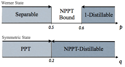
Figure 1: Entanglement properties of Werner, $\rho_{W}$, and symmetric state, $\sigma(q)$, for the qutrit case ($d=3$). In the region between separability and 1-distillability, $\rho_{W}$ is NPPT and conjectured bound. The point $q=0.2$ represents the extremal value for which states $\sigma(q)$ are PPT, thus not distillable. For larger values of $q$ the states are distillable (in particular, 1-distillable).

2.1.2 Protocol for Quantum Activation

As already announced, any entangled Werner state, and in particular any conjectured bound entangled Werner state, gives a distillable state when combined with the universal activator $\sigma(q)$ with $q=1/(d+2)$, simply denoted as $\sigma$. If initially the two parties are sharing a Werner state $\rho$ acting on $\mathcal{H}_{0}=\mathcal{H}_{A_{0}}\otimes\mathcal{H}_{B_{0}}$ and a symmetric state $\sigma$ acting on $\mathcal{H}_{1,2}=\mathcal{H}_{A_{1}}\otimes\mathcal{H}_{A_{2}}\otimes\mathcal{H}_{B_{1}}\otimes\mathcal{H}_{B_{2}}$, each party applies a projection onto a maximally entangled states on $\mathcal{H}_{A_{0}}\otimes\mathcal{H}_{A_{1}}$ and $\mathcal{H}_{B_{0}}\otimes\mathcal{H}_{B_{1}}$ respectively. The resulting state is an isotropic state $\rho_{iso}$ acting on $\mathcal{H}_{A_{2}}\otimes\mathcal{H}_{B_{2}}$. Recall that isotropic state are $U\otimes U^{*}$ invariant and defined by the convex combination of a maximally entangled state and white noise, $\operatorname{\mathbb{I}}/d^{2}$. One can see that the resulting isotropic state has an overlap with a maximally entangled state, $\mathrm{tr}(\rho_{iso}\mathds{P}_{d})$, larger than $1/d$ for any entangled Werner state. As shown in [33], this condition is sufficient for distillability.

2.2 Classical Activation

This section contains the main results of our work. Our goal is to construct a classical cryptographic analog of the quantum activation example discussed above.

We first associate probability distributions to all the previous quantum states. In order to do so, we purify the initial bipartite noisy quantum states $\rho_{AB}$ by including an environment, and then map the tripartite quantum states $|\psi_{ABE}\rangle$ onto probability distributions by performing some local measurements, see (5). The procedure to choose these measurements is always the same: computational bases for the honest parties, and general measurements for Eve. More precisely, denoting by $X$ and $Y$ the result obtained by Alice and Bob, this effectively projects Eve’s system onto the pure state $|e_{XY}\rangle=\langle XY|\psi_{ABE}\rangle$ with probability $P(XY)=\langle XY|\rho_{AB}|XY\rangle$. Given that, the measurement that Eve applies is the one that minimizes her error probability when distinguishing the states in the ensemble $\{|e_{XY}\rangle,P(XY)\}$. Note that this choice of measurement may not necessarily be optimal from Eve’s point of view in terms of the secret correlations between Alice and Bob, but it seems a natural choice. This procedure is applied to the two family of states, namely Werner and symmetric. Because of the symmetries of these states, the measurements minimizing Eve’s error probability can be analytically determined using the results of Refs [34, 35].

In order to characterize the secrecy properties of the obtained probability distributions, we compute the intrinsic information when numerically possible and use AD protocols for distillability. We stress that the considered protocols distill a secret key in the same region of parameters in which entanglement distillation was possible for the initial quantum states. Finally, we introduce a quantum-like activation protocol that maps the two probability distributions into a new distribution in which Alice and Bob each have a bit. We then prove that an AD protocol allows distilling a secret key for some value of the parameters in which the initial quantum states were non-distillable. However, we are unable to close all the gap between entanglement and 1-distillability for the Werner state.

2.2.1 Probability Distributions

Werner states distribution. We start by mapping the Werner states of two qutrits onto a probability distribution $P_{XYZ}$ following the recipe explained in the previous section. In this way, we get a one-parameter family of probability distributions $P_{XYZ}$, (see Table 1 for details), which depends just on the same parameter $p$ defining the initial Werner state (6). The resulting distributions are given in Table 1. The indices for Eve’s symbols specify her guess on Alice’s and Bob’s symbols or, in other words, if Eve outcome is $Z=z_{ij}$, the most probable outcomes for Alice and Bob are $X=i$ and $Y=j$.

$$\begin{array}[]{c||c|c|c|}&0&1&2\bigstrut[b]\\ \hline\cr\hline\cr 0&\lambda_{1}\quad(z_{00})&\frac{\lambda_{1}+\lambda_{2}}{2}\begin{cases}\delta_{Z}&\textrm{$(z_{10})$}\\ 1-\delta_{Z}&\textrm{$(z_{01})$}\end{cases}&\frac{\lambda_{1}+\lambda_{2}}{2}\begin{cases}\delta_{Z}&\textrm{$(z_{20})$}\\ 1-\delta_{Z}&\textrm{$(z_{02})$}\end{cases}\bigstrut\\ \hline\cr 1&\frac{\lambda_{1}+\lambda_{2}}{2}\begin{cases}\delta_{Z}&\textrm{$(z_{01})$}\\ 1-\delta_{Z}&\textrm{$(z_{10})$}\end{cases}&\lambda_{1}\quad(z_{11})&\frac{\lambda_{1}+\lambda_{2}}{2}\begin{cases}\delta_{Z}&\textrm{$(z_{21})$}\\ 1-\delta_{Z}&\textrm{$(z_{12})$}\end{cases}\bigstrut\\ \hline\cr 2&\frac{\lambda_{1}+\lambda_{2}}{2}\begin{cases}\delta_{Z}&\textrm{$(z_{02})$}\\ 1-\delta_{Z}&\textrm{$(z_{20})$}\end{cases}&\frac{\lambda_{1}+\lambda_{2}}{2}\begin{cases}\delta_{Z}&\textrm{$(z_{12})$}\\ 1-\delta_{Z}&\textrm{$(z_{21})$}\end{cases}&\lambda_{1}\quad(z_{22})\bigstrut\\ \hline\cr\end{array}$$

Table 1: Tripartite probability distributions derived from Werner states (6). The parameters in the table are as follows: $\lambda_{1}=(1-p)/6$, $\lambda_{2}=p/3$ and $\delta_{Z}=(\sqrt{\lambda_{1}}-\sqrt{\lambda_{2}})^{2}/(2(\lambda_{1}+\lambda_{2}))$. Rows (columns) represent Alice’s (Bob’s) symbols. Eve’s symbols are shown in parenthesis. For example, the cell $(X=0,Y=1)$ shows that whenever Alice and Bob get (0,1) (which happen with probability $(\lambda_{1}+\lambda_{2})/2$), Eve correctly guesses the symbol $z_{01}$ with probability $1-\delta_{Z}$, and makes an error (symbol $z_{10}$) with probability $\delta_{Z}$.

As done for entanglement, we now characterize these distributions in terms of their secret correlations. Recall that for the quantum case and qutrits, the state was entangled for $p>p_{s}=1/2$ and conjectured non-distillable for $p\leq p_{1d}=3/5$. As we show next, the same values appear for the analogous classical distributions. Concerning the point $p_{s}$, we compute the intrinsic information of the distributions in Table 1 by numerical optimization over all possible channels by Eve. Of course, one can never exclude the existence of local minima and, therefore, that the intrinsic information is strictly smaller than what numerically obtained. One may wonder why this computation is necessary. For instance, at the point $p=p_{s}$ the quantum state is separable and, then, it is known that there exists a measurement by Eve such that the intrinsic information between Alice and Bob is zero for all measurements. Note however that in terms of intrinsic information, the optimal measurement by Eve is the one that prepares on Alice and Bob the ensemble of product states compatible with the separable state Alice and Bob share. This measurement is not necessarily the same as the one minimizing Eve’s error probability when Alice and Bob measure in the computational bases. The same applies to the entanglement region. While there are measurements such that Alice and Bob share secret correlations no matter which measurement Eve performs, these measurements are not on the computational bases.

Using the numerical insight, we find a conjectured optimal channel that reproduces the numerical results. The optimal channel gives zero intrinsic information exactly at the point $p=p_{s}$. It maps Eve’s symbols $z_{ii}$ onto $z{ij}$ with $i\neq j$ with equal probability ($i,j=0,1,2$). Its easy form leads to the following analytical expression for $I(X;Y\downarrow Z)$:

$$I(X;Y\downarrow Z)=-\log(1-x^{2})-x\log\left(\frac{1+x}{1-x}\sqrt{\frac{\tau-2x}{\tau+2x}}\right)+\frac{\tau}{4}\log{(\tau^{2}-4x^{2})}+\left(1-\frac{\tau}{2}\right)\log(2-\tau)$$

where $\tau=1+p$, $x=\sqrt{2p(1-p)}$. Figure 2 shows the behavior of this quantity in the region of interest.

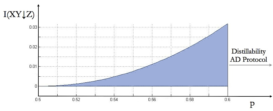
Figure 2: Behaviour of the intrinsic information for the $P_{XYZ}$ relative to the Werner state. Note that: i) $I(X;Y\downarrow Z)$ is equal to $0$ at point $p=0.5$ which corresponds to the last point of separability for the Werner state; ii) $I(X;Y\downarrow Z)$ is strictly positive at point $p=0.6$ which corresponds to the extreme value of $p$ for which it is 1-copy distillable.

Moving to the distillability properties, we study AD protocols and identify a value of $p$ for which positive secret-key rate can be obtained by the two honest parties through these protocols. The considered protocol is the quantum analogue of the quantum one and uses a binaryzation. Alice and Bob first discard one (but the same) of their symbols. Then, one of the parties, say Bob, applies a local permutation to his symbols. For example, if they agreed on discarding symbol 2, then Bob applies $0\leftrightarrow 1$. Alice and Bob now apply AD to the resulting two-bit distribution. This distribution is shown in Table 2.

From the obtained table, it is possible to estimate the dependence of Bob’s and Eve’s errors on the size of the blocks used for AD, denoted by $N$. Recall that in the case of bits the protocols works as follows: Alice generates a random bit $\zeta$ and chooses $N$ symbols ${\bf a}$ from her list of data. She then sends to Bob the information about these symbols and the vector ${\bf\bar{a}}$ such that $a_{i}\oplus\bar{a}_{i}=\zeta,\forall i$. Bob takes the symbols in his list corresponding to those chosen by Alice, ${\bf b}$, and accepts only when $\chi=b_{i}\oplus\bar{a}_{i},\forall i$. Bob’s error probability $\beta_{N}$ is now easy to compute. Denote by $\beta$ the error probability in the initial two-bit probability distribution, $\beta=P(X\neq Y)=2\lambda_{1}/(3\lambda_{1}+\lambda_{2})$. Bob accepts a bit whenever either all his $N$ symbols are identical to those of Alice, which happens with probability $(1-\beta)^{N}$, or all his symbols are different, whose probability is $\beta^{N}$. Thus, the probability of accepting a wrong bit conditioned on acceptance is given by:

$$\beta_{N}=\frac{\beta^{N}}{\beta^{N}+(1-\beta)^{N}}\leqslant\left(\frac{\beta}{1-\beta}\right)^{N}.$$ (8)

The upper bound becomes tight in the limit $N\rightarrow\infty$.

$$\begin{array}[]{c||c|c|}&0&1\bigstrut[b]\\ \hline\cr\hline\cr 0&\frac{\lambda_{1}+\lambda_{2}}{2}\begin{cases}\delta_{Z}&\textrm{$(z_{11})$}\\ 1-\delta_{Z}&\textrm{$(z_{00})$}\end{cases}&\lambda_{1}\quad(z_{01})\bigstrut\\ \hline\cr 1&\lambda_{1}\quad(z_{10})&\frac{\lambda_{1}+\lambda_{2}}{2}\begin{cases}\delta_{Z}&\textrm{$(z_{00})$}\\ 1-\delta_{Z}&\textrm{$(z_{11})$}\end{cases}\bigstrut\\ \hline\cr\end{array}$$

Table 2: Two-bit distribution resulting from projecting the initial distribution of Table 1 on the space $X,Y=0,1$ and after Bob permutes his symbol. For the sake of clarity, we apply a permutation also on the second index of Eve’s symbols, that is $z_{ij}\rightarrow z_{i1-j}$. All the terms in the table should be normalized by a factor $3\lambda_{1}+\lambda_{2}$.

We now move to the estimation of Eve’s error $\epsilon_{N}$. As her information is probabilistic, there is always a non-zero probability that she makes a mistake. For the estimation we compute a lower bound on the error given by all the cases in which the $N$ symbols observed by Eve do not provide her any information about the value of the bit generated by Alice. In the computation, it is simpler to use Eve’s probabilities conditioned on the fact that Alice and Bob have made no mistake after AD (which means that no mistake has occurred for any of the $N$ symbols). Or in other words, we only consider the terms in the diagonal of Table 2. This does not make any difference for what follows as in the limit $N\rightarrow\infty$ the probability of Bob accepting a wrong symbol goes to zero. After Bob’s acceptance, Eve knows that the actual string ${\bf a}$ used by Alice is either equal to $\bar{{\bf a}}$ (the one sent on the public channel) when $\zeta=0$, or ${\bf\bar{a}}^{\prime}$ (the permuted one, that is, $\bar{a}^{\prime}_{i}=1-\bar{a}_{i}$) when $\zeta=1$. Clearly, all the events in which the $N$ symbols observed by Eve, $Z^{(i)}$, are such that $P(Z^{(1)}..\ Z^{(N)}|{\bf a}=\bar{{\bf a}})=$ $P(Z^{(1)}..\ Z^{(N)}|{\bf a}={\bf\bar{a}}^{\prime})$ do not give her any information about $\zeta$. In these cases, Eve has to randomly guess Alice’s symbol and makes an error with probability $1/2$. Due to the symmetry in the diagonal of Table 2, that is, $P(Z=z_{00}|X=0)=P(Z=z_{11}=1|X=1)$ and $P(Z=z_{11}|X=0)=P(Z=z_{00}|X=1)$, all the events where Eve has exactly $N/2$ of her symbols equal to $z_{00}$ and $N/2$ equal to $z_{11}$ satisfy the previous condition and, thus, contribute to her error. Counting all the possible ways of distributing these cases leads to the following lower bound on Eve’s error probability [36]:

$$\epsilon_{N}\geqslant\frac{1}{2}\left(\begin{array}[]{c}N\\ N/2\end{array}\right)\delta_{Z}^{N/2}(1-\delta_{Z})^{N/2}$$ (9)

where $\delta_{Z}$ is the probability for Eve to guess wrongly conditioned on those cases in which Alice and Bob’s symbols coincide (this value is made explicit in the caption of Figure 1). The asymptotic behavior of (9), after applying the Stirling’s approximation $(n!)^{2}\simeq(2n)!/2^{2n}$ and expanding the binomial coefficient can be expressed as:

$$\epsilon_{N}\geqslant c(2\sqrt{\delta_{Z}(1-\delta_{Z})})^{N},$$ (10)

with $c$ being a positive constant.

By comparing Eqs. (8) and (10) one concludes that whenever

$$\frac{\beta}{1-\beta}<2\sqrt{\delta_{Z}(1-\delta_{Z})}$$ (11)

key distillation is possible. This follows from the fact that, if this condition holds, Bob’s error is exponentially smaller than Eve’s with $N$. This in turn implies that it is possible to choose a value of $N$ such that Alice-Bob mutual information is larger than Alice-Eve and one-way distillation techniques can distill a secret key. From (10) one gets that AD works whenever $p>3/5$, as for 1-distillability in the quantum case. Before concluding this part, we would like to mention that the same range of parameters for distillation is obtained if one applies the generalized AD protocol of Ref. [27].

Symmetric states distribution. We apply the same machinery to the symmetric states $\sigma(q)$. Again, the symmetries of the states allow the explicit computation of the measurement by Eve minimizing her error probability for any value of $q$. The obtained distributions, denoted by $Q_{X1,Y1,X2,Y2,\tilde{Z}}$, is significantly more complex and shown in Appendix A. It consists of two trits for Alice, $(X_{1},X_{2})$ and two trits for Bob, $(X_{2},Y_{2})$, while Eve’s variable can take $63$ possible values. It is now much harder to estimate the secrecy properties of the distribution. For instance, we did not make any attempt to compute the intrinsic information. However, we are able to show that Alice and Bob can distill a secret key whenever $q>1/5$ as in the quantum regime.

To simplify our task, we exploit again the concept of binaryzation. Inspired by the quantum projections used for the distillation of $\sigma(q)$, Alice and Bob select two outcomes on each side, namely $00,01$ for Alice and $10,11$ for Bob. The obtained two-bit distribution is shown in Table 3.

$$\begin{array}[]{c||c|c|}&0\>[10]&1\>[11]\bigstrut[b]\\ \hline\cr\hline\cr 0\>[00]&\frac{1+7q}{5+11q}\begin{cases}P_{G}&\textrm{$(\tilde{z}_{0100})$}\\ P_{L}&\textrm{$(\tilde{z}_{0111})$}\\ P_{L}&\textrm{$(\tilde{z}_{0122})$}\\ P_{B}&\textrm{$(\tilde{z}_{1000})$}\\ P_{H}&\textrm{$(\tilde{z}_{1011})$}\\ P_{H}&\textrm{$(\tilde{z}_{1022})$}\\ \end{cases}&\frac{3(1-q)}{2(5+11q)}\begin{cases}1/2&\textrm{$(\tilde{z}_{0101})$}\\ 1/2&\textrm{$(\tilde{z}_{1001})$}\end{cases}\bigstrut\\ \hline\cr 1\>[01]&\frac{3(1-q)}{2(5+11q)}\begin{cases}1/2&\textrm{$(\tilde{z}_{0110})$}\\ 1/2&\textrm{$(\tilde{z}_{1010})$}\end{cases}&\frac{1+7q}{5+11q}\begin{cases}P_{L}&\textrm{$(\tilde{z}_{0100})$}\\ P_{G}&\textrm{$(\tilde{z}_{0111})$}\\ P_{L}&\textrm{$(\tilde{z}_{0122})$}\\ P_{H}&\textrm{$(\tilde{z}_{1000})$}\\ P_{B}&\textrm{$(\tilde{z}_{1011})$}\\ P_{H}&\textrm{$(\tilde{z}_{1022})$}\\ \end{cases}\bigstrut\\ \hline\cr\end{array}$$

Table 3: Two-bit distribution obtained as a result of the binaryzation applied to $Q_{X1,Y1,X2,Y2,\tilde{Z}}$. Note that we have relabeled the old symbols (shown in square brakets) by $0$ and $1$, in the following we use $\tilde{X},\tilde{Y}$ to refer to them. The parameters in the table are as follows: $\alpha=\sqrt{8q/(1+7q)}$ and $\gamma=\sqrt{(1-q)/(2(1+7q))}$, $P_{G}=(\alpha+2\gamma)^{2}/6$, $P_{B}=(-\alpha+2\gamma)^{2}/6$, $P_{L}=(\alpha-\gamma)^{2}/6$, $P_{H}=(\alpha+\gamma)^{2}/6$.

They apply the standard bit AD protocol to this distribution. As before, Bob’s error can be easily computed, getting the same as in Eq. (8), but now with $\beta$ equal to $3(1-q)/(5+11q)$. The estimation of Eve’s error is much more cumbersome. As above, the main idea is to derive a lower bound on it based on those instances in which Eve’s symbols do not provide her any information about the symbol $\zeta$ Alice used for AD. Again, one can restrict the analysis to the terms in the diagonal of Table 3. The main difference in comparison with the simple case discussed above is the larger number of symbols for Eve. However, given the symmetry of the distribution 3 it is enough to consider Eve’s symbols pair-wise:

$$P(\tilde{Z}=\tilde{z}_{0100}|\tilde{X}\tilde{Y}=00)=P(\tilde{Z}=\tilde{z}_{0111}|\tilde{X}\tilde{Y}=11)=\bar{\delta}_{1}$$

$$P(\tilde{Z}=\tilde{z}_{0100}|\tilde{X}\tilde{Y}=11)=P(\tilde{Z}=\tilde{z}_{0111}|\tilde{X}\tilde{Y}=00)=\bar{\eta}_{1}$$

$$P(\tilde{Z}=\tilde{z}_{1000}|\tilde{X}\tilde{Y}=00)=P(\tilde{Z}=\tilde{z}_{1011}|\tilde{X}\tilde{Y}=11)=\bar{\delta}_{2}$$

$$P(\tilde{Z}=\tilde{z}_{1000}|\tilde{X}\tilde{Y}=11)=P(\tilde{Z}=\tilde{z}_{1011}|\tilde{X}\tilde{Y}=00)=\bar{\eta}_{2}$$

where we have used $\tilde{X},\tilde{Y}$ to denote the re-labeling of Alice and Bob’s symbols. Note that the last two subindexes of Eve’s symbols are those that give her information about Alice’s (and Bob’s) symbol. Symbols $\tilde{z}_{**22}$ give her no information about Alice’s symbols, so we sum them, their total probability being $\delta_{3}$. Given the public string $\bar{{\bf a}}_{N}$, one can see that all those cases for which Eve has the same number $n_{1}$ of $\tilde{z}_{0100}$ and $\tilde{z}_{0111}$ and the same number $n_{2}$ of $\tilde{z}_{1000}$ and $\tilde{z}_{1011}$, with $N=2n_{1}+2n_{2}+2n_{3}$ and where $2n_{3}$ is the total number of symbols $\tilde{z}_{**22}$, contribute to her error. Thus, counting all these cases leads to the following lower bound on Eve’s error:

$$\epsilon_{N}\geqslant\frac{1}{2}\sum_{n_{1},n_{2},n_{3}}\frac{N!}{(2n_{1})!(2n_{2})!(2n_{3})!}\left(2\sqrt{\delta_{1}\eta_{1}}\right)^{2n_{1}}\left(2\sqrt{\delta_{2}\eta_{2}}\right)^{2n_{2}}\left(\delta_{3}\right)^{2n_{3}}$$ (12)

where $\delta_{i}$ and $\eta_{i}$ are the probabilities shown above but normalized (since as already stated we are considering the asymptotic case). After Stirling’s approximation and summing eq. (12) the following compact form is obtained:

$$\epsilon_{N}\geqslant c\left(2\sqrt{\delta_{1}\eta_{1}}+2\sqrt{\delta_{2}\eta_{2}}+\delta_{3}\right)^{N}$$

with $c$ being a positive constant. Comparing the scaling of the errors, one has that AD works whenever

$$\frac{\beta}{1-\beta}<2\sqrt{\delta_{1}\eta_{1}}+2\sqrt{\delta_{2}\eta_{2}}+\delta_{3}$$ (13)

where the right hand side is equal to $(\alpha+\gamma)^{2}/3$ (the values of $\alpha$ and $\gamma$ are reported in the caption of Table 3). Eq. (13) is hence satisfied whenever $q>\tilde{q}=0.2$, as announced.

2.2.2 Protocol for Classsical Activation

Inspired by the quantum activation example of Ref. [8], we consider the following classical protocol. Alice and Bob have access to the trits $X$ and $Y$, whose correlations are described by $P_{XYZ}$, and the two trits $(X_{1},X_{2})$ and $(Y_{1},Y_{2})$ correlated according to $Q_{X1,Y1,X2,Y2,\tilde{Z}}$. Alice (Bob) keeps $X_{2}$ ($Y_{2}$), and only $X_{2}$ ($Y_{2}$), whenever $X=X_{1}$ ($Y=Y_{1}$); otherwise they discard all the symbols. This filtering projects the initial probability into a slightly simpler two-trit distribution. The new probability distribution $Q^{*}(X_{2},Y_{2},E)$ reads:

$$Q^{*}(X_{2},Y_{2},E)=\sum_{x,y=0}^{2}P(X=x,Y=y,Z)Q(X_{1}=x,Y_{1}=y,X_{2},Y_{2},\tilde{Z})$$ (14)

where $E=[Z,\tilde{Z}]$ is the collection of Eve’s ymbols. Finally Alice and Bob binaryze their symbols by discarding one of the three values (the same for both), say 2. The resulting distribution is shown in Table 4.

As above, we use AD protocols to estimate the value of $p$ for which Alice and Bob can extract a positive secret key rate if they are sharing pairs of bits distributed according to Table 4. We are able to prove that whenever $p>p_{c}\simeq 0.513$ an AD protocol allows distilling a secret key from the distribution in Table 4 and, thus, a form of activation is possible. Unfortunately, we are unable to reach the point $p=0.5$, as in the quantum scenario. However, our analysis suggests that the secret key rate is non-additive for some values of $p$. In the following we summarize the key steps leading to this result.

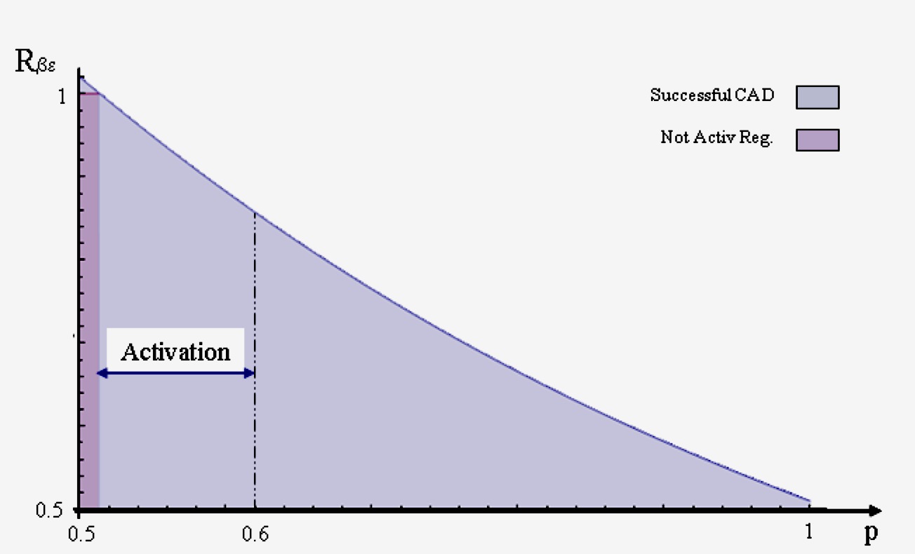
Figure 3: The CAD protocol certifies that if the Werner state distribution (Table 1) is taken with $p>0.513$ positive secrecy can be extracted by the honest parties. Unfortunately, we cannot completely close the gap up to $p=0.5$. This would have shown a direct correspondence between the quantum and the classical scenario.

$$\begin{array}[]{c||c|c|}&0&1\\ \hline\cr\hline\cr\hbox{\multirowsetup 0}&\hskip 9.95863pt\frac{\lambda_{1}(1-q)}{72c_{N}}\footnotesize\begin{cases}2/3\hskip 65.44142pt(z_{ii},\tilde{z}_{ii00})\\ 1/6\hskip 65.44142pt(z_{ii},\tilde{z}_{ii11})\\ 1/6\hskip 65.44142pt(z_{ii},\tilde{z}_{ii22})\\ \end{cases}&\hskip 19.91684pt\frac{\lambda_{1}(1-q)}{48c_{N}}\footnotesize\begin{cases}1\hskip 36.98866pt(z_{00},\tilde{z}_{0001})\\ 1\hskip 36.98866pt(z_{11},\tilde{z}_{1101})\\ 1\hskip 36.98866pt(z_{22},\tilde{z}_{2201})\\ \end{cases}\\ &\frac{(\lambda_{1}+\lambda_{2})s_{N}}{2}\footnotesize\begin{cases}\delta_{Z}P_{G}+(1-\delta_{Z})P_{B}\hskip 2.84544pt(z_{ts},\tilde{z}_{st00})\\ \delta_{Z}P_{L}+(1-\delta_{Z})P_{H}\hskip 2.84544pt(z_{ts},\tilde{z}_{st11})\\ \delta_{Z}P_{L}+(1-\delta_{Z})P_{H}\hskip 2.84544pt(z_{ts},\tilde{z}_{st22})\\ \delta_{Z}P_{B}+(1-\delta_{Z})P_{G}\hskip 2.84544pt(z_{ts},\tilde{z}_{ts00})\\ \delta_{Z}P_{H}+(1-\delta_{Z})P_{L}\hskip 2.84544pt(z_{ts},\tilde{z}_{ts11})\\ \delta_{Z}P_{H}+(1-\delta_{Z})P_{L}\hskip 2.84544pt(z_{ts},\tilde{z}_{ts22})\\ \delta_{Z}P_{B}+(1-\delta_{Z})P_{G}\hskip 2.84544pt(z_{st},\tilde{z}_{st00})\\ \delta_{Z}P_{H}+(1-\delta_{Z})P_{L}\hskip 2.84544pt(z_{st},\tilde{z}_{st11})\\ \delta_{Z}P_{H}+(1-\delta_{Z})P_{L}\hskip 2.84544pt(z_{st},\tilde{z}_{st22})\\ \delta_{Z}P_{G}+(1-\delta_{Z})P_{B}\hskip 2.84544pt(z_{st},\tilde{z}_{ts00})\\ \delta_{Z}P_{L}+(1-\delta_{Z})P_{H}\hskip 2.84544pt(z_{st},\tilde{z}_{ts11})\\ \delta_{Z}P_{L}+(1-\delta_{Z})P_{H}\hskip 2.84544pt(z_{st},\tilde{z}_{ts22})\\ \end{cases}&\frac{(\lambda_{1}+\lambda_{2})(1-q)}{192c_{N}}\footnotesize\begin{cases}1/2\hskip 28.45274pt(z_{01},\tilde{z}_{0101})\\ 1/2\hskip 28.45274pt(z_{01},\tilde{z}_{1001})\\ 1/2\hskip 28.45274pt(z_{10},\tilde{z}_{0101})\\ 1/2\hskip 28.45274pt(z_{10},\tilde{z}_{1001})\\ 1/2\hskip 28.45274pt(z_{02},\tilde{z}_{0201})\\ 1/2\hskip 28.45274pt(z_{02},\tilde{z}_{2001})\\ 1/2\hskip 28.45274pt(z_{20},\tilde{z}_{0201})\\ 1/2\hskip 28.45274pt(z_{20},\tilde{z}_{2001})\\ 1/2\hskip 28.45274pt(z_{12},\tilde{z}_{1201})\\ 1/2\hskip 28.45274pt(z_{12},\tilde{z}_{2101})\\ 1/2\hskip 28.45274pt(z_{21},\tilde{z}_{1201})\\ 1/2\hskip 28.45274pt(z_{21},\tilde{z}_{2101})\\ \end{cases}\\ \hline\cr\hbox{\multirowsetup 1}&\hskip 19.91684pt\frac{\lambda_{1}(1-q)}{48c_{N}}\footnotesize\begin{cases}1\hskip 36.98866pt(z_{00},\tilde{z}_{0010})\\ 1\hskip 36.98866pt(z_{11},\tilde{z}_{1110})\\ 1\hskip 36.98866pt(z_{22},\tilde{z}_{2210})\\ \end{cases}&\hskip 8.5359pt\frac{\lambda_{1}(1-q)}{72c_{N}}\footnotesize\begin{cases}1/6\hskip 65.44142pt(z_{ii},\tilde{z}_{ii00})\\ 2/3\hskip 65.44142pt(z_{ii},\tilde{z}_{ii11})\\ 1/6\hskip 65.44142pt(z_{ii},\tilde{z}_{ii22})\\ \end{cases}\\ &\frac{(\lambda_{1}+\lambda_{2})(1-q)}{192c_{N}}\footnotesize\begin{cases}1/2\hskip 28.45274pt(z_{01},\tilde{z}_{0110})\\ 1/2\hskip 28.45274pt(z_{01},\tilde{z}_{1010})\\ 1/2\hskip 28.45274pt(z_{10},\tilde{z}_{0110})\\ 1/2\hskip 28.45274pt(z_{10},\tilde{z}_{1010})\\ 1/2\hskip 28.45274pt(z_{02},\tilde{z}_{0210})\\ 1/2\hskip 28.45274pt(z_{02},\tilde{z}_{2010})\\ 1/2\hskip 28.45274pt(z_{20},\tilde{z}_{0210})\\ 1/2\hskip 28.45274pt(z_{20},\tilde{z}_{2010})\\ 1/2\hskip 28.45274pt(z_{12},\tilde{z}_{1210})\\ 1/2\hskip 28.45274pt(z_{12},\tilde{z}_{2110})\\ 1/2\hskip 28.45274pt(z_{21},\tilde{z}_{1210})\\ 1/2\hskip 28.45274pt(z_{21},\tilde{z}_{2110})\\ \end{cases}&\frac{(\lambda_{1}+\lambda_{2})s_{N}}{2}\footnotesize\begin{cases}\delta_{Z}P_{L}+(1-\delta_{Z})P_{H}\hskip 2.84544pt(z_{ts},\tilde{z}_{st00})\\ \delta_{Z}P_{G}+(1-\delta_{Z})P_{B}\hskip 2.84544pt(z_{ts},\tilde{z}_{st11})\\ \delta_{Z}P_{L}+(1-\delta_{Z})P_{H}\hskip 2.84544pt(z_{ts},\tilde{z}_{st22})\\ \delta_{Z}P_{H}+(1-\delta_{Z})P_{L}\hskip 2.84544pt(z_{ts},\tilde{z}_{ts00})\\ \delta_{Z}P_{B}+(1-\delta_{Z})P_{G}\hskip 2.84544pt(z_{ts},\tilde{z}_{ts11})\\ \delta_{Z}P_{H}+(1-\delta_{Z})P_{L}\hskip 2.84544pt(z_{ts},\tilde{z}_{ts22})\\ \delta_{Z}P_{H}+(1-\delta_{Z})P_{L}\hskip 2.84544pt(z_{st},\tilde{z}_{st00})\\ \delta_{Z}P_{B}+(1-\delta_{Z})P_{G}\hskip 2.84544pt(z_{st},\tilde{z}_{st11})\\ \delta_{Z}P_{H}+(1-\delta_{Z})P_{L}\hskip 2.84544pt(z_{st},\tilde{z}_{st22})\\ \delta_{Z}P_{L}+(1-\delta_{Z})P_{H}\hskip 2.84544pt(z_{st},\tilde{z}_{ts00})\\ \delta_{Z}P_{G}+(1-\delta_{Z})P_{B}\hskip 2.84544pt(z_{st},\tilde{z}_{ts11})\\ \delta_{Z}P_{L}+(1-\delta_{Z})P_{H}\hskip 2.84544pt(z_{st},\tilde{z}_{ts22})\\ \end{cases}\\ \hline\cr\end{array}$$

Table 4: Resulting tripartite distribution after the application of the classical protocol by the two honest parties. The initial probability distributions $P_{XYZ}$ and $Q_{X1,Y1,X2,Y2,\tilde{Z}}$ are mapped to the new probability distribution $Q^{*}(X_{2},Y_{2},E)$ shown above. From this classical object we can derive the minimum value of $p$ for which positive secret key can be extracted by A and B. The parameters that appear above are expressed as a function of p and q, the two key parameters in the initial probability distributions. $c_{N}=(\lambda_{1}+\lambda_{2})(5+11q)/48+5\lambda_{1}(1-q)/24$, $s_{N}=(1+7q)/(144c_{N})$, $i,s,t=0,1,2$ with $s\neq t$ and $s<t$. In our procedure the optimal $q$ for the symmetric state distribution is taken equal to $1/5$.

As mentioned, the values of interest for $P_{XYZ}$ and $Q_{X1,Y1,X2,Y2,\tilde{Z}}$ are, $0.5<p\leqslant 0.6$ and $q=0.2$, respectively. The distribution $Q^{*}(X_{2},Y_{2},E)$ resulting from the local filtering by the honest parties depends on the parameter $p$. In order to estimate Eve’s error we follow a similar argument as for $Q_{X1,Y1,X2,Y2,\tilde{Z}}$, now adapted to this slightly more complex case. Despite the big amount of symbols on Eve’s side (see Table 4), the symmetry in the distribution leads to six main classes that are relevant for the AD analysis (appendix B further clarifies this point). These arguments lead to the following bound on Eve’s error:

$$\epsilon_{N}\geqslant\frac{1}{2}\sum_{n_{1},n_{2}\ldots n_{6}}\frac{N!}{(2n_{1})!\ldots(2n_{6})!}\left(6\sqrt{\delta_{1}\ \eta_{1}}\ \right)^{2n_{1}}\dots\left(6\sqrt{\delta_{5}\ \eta_{5}}\right)^{2n_{5}}\delta_{6}^{2n_{6}}$$ (15)

where $\sum^{6}_{i=1}2n_{i}=N$. Note that as before the terms $\delta_{i}\eta_{i}$ with $i=1\ldots 5$ take into account those cases in which Eve has $n_{i}$ symbols that coincide with the public string sent by Alice and $n_{i}$ symbols that are opposite to those appearing in the public string. The last term, $\delta_{6}$, as before, refers to the sum of probabilities for which Eve has no information at all (see details in appendix B). In the asymptotic case we are treating here, Eq. (15) converges to a multinomial distribution, namely:

$$\epsilon_{N}\geqslant c\left(6\left(\sqrt{\delta_{1}\ \eta_{1}}\ +\dots\sqrt{\delta_{5}\ \eta_{5}}\right)+\delta_{6}\right)^{N}$$ (16)

with $c$ being a positive constant. Bob’s error is much easier to compute, getting $\beta=(3\lambda_{1}+\lambda_{2})(1-q)/(16c_{N})$. Putting these two terms together, we have that the AD protocols works whenever:

$$\frac{\beta}{1-\beta}<6\left(\sqrt{\delta_{1}\ \eta_{1}}\ +\dots\sqrt{\delta_{5}\ \eta_{5}}\right)+\delta_{6}$$ (17)

Figure 3 shows the ratio between the left hand side and the right hand side, $R_{\beta\epsilon}$, as a function of the parameter $p$. As above, whenever $R_{\beta\epsilon}<1$, the AD protocol succeeds. The point at which $R_{\beta\epsilon}=1$ corresponds to $p=0.513$, as already announced.

3 Conclusions

Non-additivity is an ubiquitous phenomenon in Quantum Information Theory due to the presence of entanglement. In this work, we provide some evidence for the existence of similar effects for secret classical correlations. Exploiting the analogies between the entanglement and secret-key agreement scenario, we have shown that two classical distributions from which no secrecy can be extracted by AD protocols can lead to a positive secret key rate when combined.

The evidence we provide is somehow similar to the conjectured example of activation for bipartite entangled states. Note however that, in the quantum case, one of the two states is provably bound. As mentioned several times, it could well happen that one, or even the two probability distributions considered here are key-distillable. Indeed, there exist examples of bound entangled states from which one can obtain probability distributions with positive secret-key rate [37]. Note however that all the known examples of bound entangled states with non-zero privacy are based on the existence of ancillary systems on the honest parties, known as shields, that prevent Eve from having the purification of the systems Alice and Bob measure to construct the key. If any of the probability distributions constructed here were key distillable, they would constitute a novel example of secret correlations from a bound entangled state that does not fit in the construction of [37].

Acknowledgement

We thank Lluis Masanes for contributions at early stages of this project. This work was supported by the ERC starting grant PERCENT, the European EU FP7 Q-Essence and QCS projects, the Spanish FIS2010-14830, Consolider-Ingenio QOIT and Chist-Era DIQIP projects.

Appendix A

This appendix shows the probability distribution obtained by Alice, Bob and Eve after measuring the symmetric state (7). Being the table very big we try to give here a schematic representation of it which can be equivalently useful to the reader to follow our arguments. It reads:

$$\begin{array}[]{c||c|c|c||c|c|c||c|c|c|}&00&01&02&10&11&12&20&21&22\bigstrut[v]\\ \hline\cr\hline\cr 00&(1_{u})&+&+&(2_{u})&*&*&(2_{w})&*&*\\ \hline\cr 01&+&(1_{u})&+&*&(2_{u})&*&*&(2_{w})&*\\ \hline\cr 02&+&+&(1_{u})&*&*&(2_{u})&*&*&(2_{w})\\ \hline\cr\hline\cr 10&(2_{u})&*&*&(1_{v})&+&+&(2_{v})&*&*\\ \hline\cr 11&*&(2_{u})&*&+&(1_{v})&+&*&(2_{v})&*\\ \hline\cr 12&*&*&(2_{u})&+&+&(1_{v})&*&*&(2_{v})\\ \hline\cr\hline\cr 20&(2_{w})&*&*&(2_{v})&*&*&(1_{w})&+&+\\ \hline\cr 21&*&(2_{w})&*&*&(2_{v})&*&+&(1_{w})&+\\ \hline\cr 22&*&*&(2_{w})&*&*&(2_{v})&+&+&(1_{w})\bigstrut\\ \hline\cr\end{array}$$

Table 5: Schematic view of the distribution $Q_{X1,Y1,X2,Y2,\tilde{Z}}$. Due to the lack of space, cells have been grouped in terms of probability distributions and number of elements (symbols) as explained below.

The joint probabilities $P(X_{1}=i,Y_{1}=k,X_{2}=j,Y_{2}=l)$ between the honest parties are distributed as follows:

• cells of type $(1_{i})$, with $i=u,v,w$ are equal to $\frac{1-q}{72}$

• cells of type $(2_{i})$, with $i=u,v,w$, are equal to $\frac{1+7q}{144}$;

• cells of type $*$ , are equal to $\frac{1-q}{48}$;

• cells of type $+$ , are equal to $\frac{1-q}{96}$;

Concerning Eve’s side (see caption of Table 1 for more details about how to read the tables):

• cells of type $(1_{i})$, with $i=u,v,w$ contain three elements. The terms that play a role in her discrimination are indicated by the same number and subindex letter. For example, consider the cell $X_{1}=0,Y_{1}=0,X_{2}=0,Y_{2}=0$. The label $1_{u}$ is used for this cell (the same one indicates $X_{1}=0,Y_{1}=0,X_{2}=1,Y_{2}=1$ and $X_{1}=0,Y_{1}=0,X_{2}=2,Y_{2}=2$). The three elements here are the three probability distributions:

  $P(0,0,0,0,\bar{z}_{00,00}),\quad P(0,0,0,0,\bar{z}_{00,11}),\quad P(0,0,0,0,\bar{z}_{00,22}).$

  $P(0,0,0,0,\bar{z}_{00,00})$ refers to the probability that Eve guesses correctly, the remaining two $P(0,0,0,0,\bar{z}_{00,11})$, $P(0,0,0,0,\bar{z}_{00,22})$ refers to the probability she guesses wrongly.

• cells of type $(2_{i})$, with $i=u,v,w$, contain six elements;

• cells of type $*$ , contain two elements distributed with probability one half (in this cases, she knows nothing about A and B symbols) ;

• cells of type $+$ , contains only one term since in this case Eve’s symbol is perfectly correlated with those of A and B;

Appendix B

In this second appendix, we clarify why it is enough to consider six classes of distributions in the AD analysis of section 2.2.2. From Table 4 the following relations hold:

$$P(E=[z_{ii},\tilde{z}_{ii00}]|X_{2}Y_{2}=00)=P(E=[z_{ii},\tilde{z}_{ii11}]|X_{2}Y_{2}=11)=\bar{\delta}_{1}$$

$$P(E=[z_{ii},\tilde{z}_{ii11}]|X_{2}Y_{2}=00)=P(E=[z_{ii},\tilde{z}_{ii00}]|X_{2}Y_{2}=11)=\bar{\eta}_{1}$$

$$P(E=[z_{ts},\tilde{z}_{st00}]|X_{2}Y_{2}=00)=P(E=[z_{ts},\tilde{z}_{st11}]|X_{2}Y_{2}=11)=\bar{\delta}_{2}$$

$$P(E=[z_{ts},\tilde{z}_{st11}]|X_{2}Y_{2}=00)=P(E=[z_{ts},\tilde{z}_{st00}]|X_{2}Y_{2}=11)=\bar{\eta}_{2}$$

$$P(E=[z_{ts},\tilde{z}_{ts00}]|X_{2}Y_{2}=00)=P(E=[z_{ts},\tilde{z}_{ts11}]|X_{2}Y_{2}=11)=\bar{\delta}_{3}$$

$$P(E=[z_{ts},\tilde{z}_{ts11}]|X_{2}Y_{2}=00)=P(E=[z_{ts},\tilde{z}_{ts00}]|X_{2}Y_{2}=11)=\bar{\eta}_{3}$$

$$P(E=[z_{st},\tilde{z}_{st00}]|X_{2}Y_{2}=00)=P(E=[z_{st},\tilde{z}_{st11}]|X_{2}Y_{2}=11)=\bar{\delta}_{4}$$

$$P(E=[z_{st},\tilde{z}_{st11}]|X_{2}Y_{2}=00)=P(E=[z_{st},\tilde{z}_{st00}]|X_{2}Y_{2}=11)=\bar{\eta}_{4}$$

$$P(E=[z_{st},\tilde{z}_{ts00}]|X_{2}Y_{2}=00)=P(E=[z_{st},\tilde{z}_{ts11}]|X_{2}Y_{2}=11)=\bar{\delta}_{5}$$

$$P(E=[z_{st},\tilde{z}_{ts11}]|X_{2}Y_{2}=00)=P(E=[z_{st},\tilde{z}_{ts00}]|X_{2}Y_{2}=11)=\bar{\eta}_{5}$$

and $\bar{\delta}_{6}$ is the sum of all the $P(E=[z_{**},\tilde{z}_{**22}]|X_{2}=Y_{2})$. As already stated in the caption of Table 4, $i,s,t=0,1,2$ with $s\neq t$ and $s<t$. In the computation, it is simpler to use Eve’s probabilities conditioned on the fact that Alice and Bob have made no mistake after AD, so this means that we only need to consider the terms in the diagonal of Table 4. For this reason the $\delta_{i},\eta_{i}$ appearing in eq. (15) are the previous ones but normalized. The complete expression is then derived according to the argument already presented at page 12.

References

- [1] C. E. Shannon, Bell System Technical Journal, vol. 27, pp.379-423 and 623-656, (1948).
- [2] G. Smith and J. Yard, Science 321, 1812 - 1815 (2008).
- [3] M. Hastings, Nature Phys. 5, 255-257 (2009).
- [4] K. Li, A. Winter, X. Zou, and G Guo, Phys. Rev. Lett. 103, 120501 (2009).
- [5] P. W. Shor, J. A. Smolin, and A. V. Thapliyal, Phys. Rev. Lett. 90, 107901 (2003).
- [6] P. Horodecki, M. Horodecki and R. Horodecki, Phys. Rev. Lett. 82 1056-1059, (1999).
- [7] P. W. Shor, J. A. Smolin and B. M. Theral, Phys. Rev. Lett. 86, 2681 (2001).
- [8] K. G. Vollbrecht and M. M. Wolf, Phys. Rev. Lett. 88, 247901 (2002).
- [9] A. Acin, J. I. Cirac, and Ll. Masanes, Phys. Rev. Lett.92 107903 (2004); Ll. Masanes and A. Acin, IEEE Trans.Inf. Theory 52, 4686 (2006).
- [10] G. Prettico and J. Bae, Phys. Rev. A 83, 042336 (2011).
- [11] N. Gisin, R. Renner, and S. Wolf, Algorithmica 34, 389 (2002).
- [12] N. Gisin and S. Wolf, Advances in Cryptology - Proceedings of Crypto 2000, Lecture Notes in Computer Science, Vol.1880, pp. 482-500 (2000).
- [13] C. H. Bennett, Phys. Today, 48 (10), 24 (1995).
- [14] C. H. Bennett, H. J. Bernstein, S. Popescu, and B. Schumacher, Phys. Rev. A 53, 2046 (1996).
- [15] P. M. Hayden, M. Horodecki, and B. M. Terhal, J. Phys. A 34, 6891 (2001).
- [16] C. H. Bennett, D. P. DiVincenzo, J. A. Smolin, and W. K. Wootters, Phys. Rev. A 54, 3824 (1996).
- [17] M. Horodecki, P. Horodecki, and R. Horodecki, Phys. Rev. Lett. 80, 5239 (1998).
- [18] A. Peres, Phys. Rev. Lett. 77,1413 (1996).
- [19] W. Dür, J. I. Cirac, M. Lewenstein and D. Bruß Phys. Rev. A, 61, 0262313 (2000).
- [20] D. P. DiVincenzo, P. W. Shor, J. A. Smolin, B. M. Theral and A.V. Thapliyal, Phys. Rev. A 61, 062312 (2000).
- [21] J. Watrous, Phys. Rev. Lett. 93, 010502 (2004).
- [22] M. Horodecki, P. Horodecki and R. Horodecki, Phys. Lett. A 223, 1 (1996).
- [23] R. Renner and W. Wolf, Advances in Cryptology, EUROCRYPT 2003, Lecture Notes in Computer Science Vol. 2656 (Springer-Verlag, Berlin, 2003), p. 562.
- [24] U. Maurer and S. Wolf, Unconditionally secure key agreement and the intrinsic conditional information, IEEE Transactions of Information Theory, Vol. 45, no 2, pp 499-514 (1999).
- [25] M. Christandl, R. Renner, and S. Wolf A property of the intrinsic mutual information, in Proceedings of International Symposium on Information Theory (ISIT) 2003, (2003).
- [26] U. M. Maurer, Secret key agreement by public discussion from common information, IEEE Transactions of Information Theory, Vol. 39, no 3, pp 733-742 (1993).
- [27] A. Acin, N. Gisin and V. Scarani, Security bounds in Quantum Cryptography using d-level systems Quant. Inf. Comp. Vol.3 No. 6, 563 (2003)
- [28] M. Curty, M. Lewenstein, and N. Lutkenhaus, Phys. Rev. Lett. 92, 217903 (2004).
- [29] A. Acin and N. Gisin, Phys. Rev. Lett. 94, 020501 (2005).
- [30] R. F. Werner, Phys. Rev. A 40, 4277 (1989).
- [31] K. G. H. Vollbrecht and R. F. Werner, Phys. Rev. A 64, 062307 (2001).
- [32] K. G. Vollbrecht and R. F. Werner, Phys. Rev. A 64, 062307 (2001).
- [33] M. Horodecki and P. Horodecki, Phys. Rev. A 59, 4206 (1999).
- [34] C. W. Helstrom, Quantum detection and estimation theory (Academic Press, New York 1976).
- [35] Y. C. Eldar, G. D. Forney Jr, IEEE Trans. Inform. Theory, vol. 47, pp. 858-872, Mar. 2001
- [36] N. Gisin and S. Wolf, Phys. Rev. Lett. 83, 4200 (1999).
- [37] K. Horodecki, M. Horodecki, P. Horodecki, J. Oppenheim, Phys. Rev. Lett. 94, 160502 (2005).