Influence of gas compression on flame acceleration in the early stage of burning in tubes

Abstract

The mechanism of finger flame acceleration at the early stage of burning in tubes was studied experimentally by Clanet and Searby [Combust. Flame 105: 225 (1996)] for slow propane-air flames, and elucidated analytically and computationally by Bychkov et al. [Combust. Flame 150: 263 (2007)] in the limit of incompressible flow. We have now analytically, experimentally and computationally studied the finger flame acceleration for fast burning flames, when the gas compressibility assumes an important role. Specifically, we have first developed a theory through small Mach number expansion up to the first-order terms, demonstrating that gas compression reduces the acceleration rate and the maximum flame tip velocity, and thereby moderates the finger flame acceleration noticeably. This is an important quantitative correction to previous theoretical analysis. We have also conducted experiments for hydrogen-oxygen mixtures with considerable initial values of the Mach number, showing finger flame acceleration with the acceleration rate much smaller than those obtained previously for hydrocarbon flames. Furthermore, we have performed numerical simulations for a wide range of initial laminar flame velocities, with the results substantiating the experiments. It is shown that the theory is in good quantitative agreement with numerical simulations for small gas compression (small initial flame velocities). Similar to previous works, the numerical simulation shows that finger flame acceleration is followed by the formation of the “tulip” flame, which indicates termination of the early acceleration process.

Keywords: premixed flames, flame acceleration, compressibility, finger flames, tulip flames

Nomenclature

$c_{S}$	sound speed
$C_{P}$	heat capacity at constant pressure
$C_{V}$	heat capacity at constant volume
$E_{a}$	activation energy
$Le$	Lewis number
$L_{f}$	flame thickness
$L_{w}$	flame length in a 2D configuration
$Ma$	initial flame propagation Mach number
$P$	pressure
$Pr$	Prandtl number
$q_{i}$	energy diffusion vector
$Q$	energy release from the reaction
$R$	tube radius (channel half-width)
$\overline{R}$	universal gas constant
$Sc$	Schmidt number
$S_{L}$	unstretched laminar burning velocity
$t$	time
$T$	temperature
$U,u$	velocity
$v$	dimensionless axial velocity
$w$	dimensionless radial velocity
$x,\ r$	radial coordinate
$Y$	mass fraction of fuel
$Z,\ z$	axial coordinate
$\alpha$	auxiliary constant
$\gamma$	adiabatic index
$\varepsilon$	total energy per unit volume
$\zeta_{i,j}$	stress tensor
$\eta$	dimensionless radial coordinate

$\Theta$	gas expansion ratio
$\vartheta$	instantaneous expansion factor
$\mu$	dynamical viscosity
$\xi$	dimensionless axial coordinate
$\rho$	density
$\sigma$	scaled acceleration rate
$\tau$	scaled time ($\tau=S_{L}t/R$)
$\tau_{R}$	factor of time dimension

Subscripts and other designations $0$ initial $pl$ planar geometry $axi$ axisymmetric geometry $b$ burnt gas $C$ modified $f$ flame, flame skirt $s$ sidewall $s,f$ just ahead of the flame skirt $s,b,f$ in the burnt gas at the flame skirt $sph$ instant/locus of shape change $tip$ flame tip $u$ unburnt mixture $w$ wave $wall$ flame touches side walls of tube $\tilde{}$ scaled value

1 Introduction

The spontaneous acceleration of a flamefront propagating from the closed end of a tube is a key element in deflagration-to-detonation transition (DDT) Zeldovich.et.al.-1985 ; Law-2006 ; Dorofeev-2011 ; Roy-et-al-review ; Dorofeev-Cicarelli-review , with two main mechanisms identified as possible causes for the flame acceleration, namely the mechanisms of Shelkin Shelkin and Bychkov et al. Bychkov.et.al-2008 for flame propagation in smooth and obstructed tubes respectively. According to the Shelkin mechanism, flames accelerate in smooth tubes due to the non-slip boundary conditions at the walls. Quantitative theory of the process has been developed and validated by extensive numerical simulations in Refs. Bychkov.et.al-2005 ; Akkerman.et.al-2006 . For the Bychkov mechanism, the delayed burning between the obstacles in obstructed tubes produces a powerful jet flow driving an extremely fast flame acceleration in the unobstructed, central portion of the tube Bychkov.et.al-2008 ; Valiev.et.al-2010 .

In addition to these two major mechanisms, another possible scenario of flame acceleration in tubes has been demonstrated experimentally by Clanet and Searby Clanet.Searby-1996 . The mechanism Clanet.Searby-1996 describes the early stage burning of a flame ignited at the center of the end face of a closed tube, leading to the transition of an initially hemi-spherical flame kernel into a finger shaped front as illustrated in Fig. 1. The tip of this finger flame experiences short but powerful acceleration until the flame skirt touches the tube walls. Thereafter, the flame acceleration stops, the flame skirt catches up with the tip rapidly and the flame inverts into a “tulip” shape. This finger flame acceleration phenomenon was first studied in the context of the “tulip flame” formation Clanet.Searby-1996 . However, it was pointed out in Refs. Bychkov.et.al-2007 ; Dorofeev-2011 that the notion of a “tulip flame” is too ambiguous, because it may be attributed to any concave flame front with a cusp pointing to the burnt region, as demonstrated by several combustion phenomena of different physical nature Xiao.et.al-2011 ; Xiao.et.al-2012 ; Oppenheim.Ghoniem-1983 ; Nkonga.et.al-1993 ; Pizza.et.al-2010 . In particular, accelerating turbulent flames in tubes/channels with no-slip at the walls, laminar Bychkov.et.al-2005 ; Akkerman.et.al-2006 or turbulent Dorofeev-2011 , also exhibit an irregular “tulip” flame shape. Furthermore, a tulip-like flame shape is also relevant to oscillating flames Gonzalez.et.al-1992 ; Gonzalez-1996 ; Petchenko.et.al-2006 ; Petchenko.et.al-2007 ; Akkerman.et.al-2006-2 ; Akkerman.et.al-2010 . To avoid any ambiguity, and recognizing that oscillating flames imply non-slip at the walls and relatively long flame propagation Akkerman.et.al-2006 ; Akkerman.et.al-2010 , in the present paper we focus only on the the laminar finger flame acceleration during the initial stage of burning, without considering other manifestations of tulip flames. The acceleration appears to proceed in a clearly exponential manner, as shown in a number of works Clanet.Searby-1996 ; Kuznetsov.et.al-2010 ; Bychkov.et.al-2007 . This is an important effect for subsequent DDT, since powerful precursor acceleration may create a leading shock wave responsible for pre-heating of the fuel mixture.

A quantitative theory of finger flame acceleration in cylindrical tubes was developed in Ref. Bychkov.et.al-2007 by assuming incompressible flow. The theory shows that the maximum velocity in the laboratory reference frame achieved by an accelerating flame tip is $(2\Theta-1)\Theta S_{L}$, where $S_{L}$ is the planar unstretched flame speed and $\Theta\equiv\rho_{u}/\rho_{b}$ the initial ratio of the fuel mixture density to the burnt gas density. For slow hydrocarbon flames with $S_{L}\approx 40$ cm/s and $\Theta\approx 8$, this yields a maximum velocity of the flame tip $\sim 120S_{L}\sim 48$ m/s, which is still considerably lower than the sound speed. The situation, however, becomes quite different for fast hydrogen-oxygen flames, with $S_{L}\lesssim 8$ m/s, $\Theta\approx 8$, and the “incompressible” estimate of Ref. Bychkov.et.al-2007 yields $(2\Theta-1)\Theta S_{L}\sim 960$ m/s, which exceeds the sound speed in the mixture, 530 m/s, and thereby fundamentally violates the incompressibility assumption. Consequently, in order to describe finger acceleration of fast flames properly, gas compressibility needs to be accounted for.

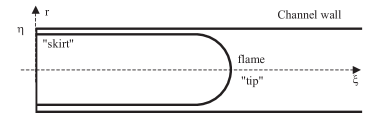
Figure 1: Geometry of an accelerating finger flame.

We next note that while the theoretical analysis predicts exponential flame acceleration with the incompressibility assumption Bychkov.et.al-2005 ; Akkerman.et.al-2006 ; Bychkov.et.al-2008 ; Valiev.et.al-2010 , various experiments showed moderation of the initial exponential regime with time and the possibility for the flame tip velocity to saturate to a supersonic speed in the laboratory reference frame Wu.et.al-2007 ; Cicarelli.et.al-2010 ; Roy-et-al-review ; Dorofeev-Cicarelli-review ; Kuznetsov.et.al-2005 . Existence of such a saturation velocity, which correlates with the Chapman-Jouguet deflagration speed, follows from the basic theory of deflagration and detonation fronts Landau.Lifshitz-1993 ; Chue-et-al-1993 . Recent numerical simulation and analytical theory demonstrated the same tendency: gas compressibility moderates the initial exponential acceleration of the flame it to a slower one, leading to saturation of the flame speed Valiev.et.al-2009 ; Valiev.et.al-2010 ; Bychkov.et.al-2010a ; Bychkov.et.al-2010b . In addition, simulations Bychkov.et.al-2008 showed that in obstructed channels fast flames with a relatively high initial Mach number exhibit noticeably lower acceleration rate as compared to slow flames. Since acceleration of finger flames has much in common with ultra-fast flame acceleration in obstructed channels Bychkov.et.al-2008 , a similar influence of gas compressibility on the finger flame acceleration is expected.

The purpose of the present paper is to study finger flame acceleration analytically, experimentally and computationally for various values of the unstretched laminar flame velocity, thus focusing on the influence of gas compressibility. The early stages of burning in tubes with slip adiabatic walls are considered. We first developed an analytical theory of flame acceleration in 2D (planar) and axisymmetric geometries through small Mach number expansion up to first-order terms, demonstrating that gas compression reduces the acceleration rate and moderates the finger flame acceleration noticeably. We then conduct experiments for hydrogen-oxygen mixtures with considerably large initial values of the Mach number, showing the scaled acceleration rate to be much smaller than that observed previously for hydrocarbon flames. We also performed numerical simulations for a wide range of initial laminar flame velocities; the results agree well with the experiments as well as the theory in the limit of small gas compression (small initial flame velocities). Similar to previous works, the numerical simulations show that the finger flame acceleration is followed by the formation of a “tulip” flame shape, which indicates the end of the early acceleration process.

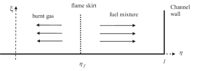
Figure 2: Flow close to the channel wall.

The paper consists of six sections. In Sections 2.1, 2.2, and 2.3 we develop the theory of flame acceleration in the early stage of burning. Details of the numerical simulations are presented in Section 3. Section 4.1 describes the experimental results. In Section 4.2 we compare results from the theory, simulation and experiment, followed by the conclusions. Resolution and laminar velocity tests are presented in the Appendix.

2 Theory of finger flame acceleration

We consider a flame front propagating in a tube/channel of radius/half-width $R$ with an ideal slip adiabatic walls as shown in Fig. 1. One end of the tube/channel is kept closed, and the embryonic flame is ignited at the central point of the closed end wall. It was explained in Refs. Bychkov.et.al-2007 ; Clanet.Searby-1996 that in the axi-symmetric, cylindrical configuration a flame front develops from a hemi-spherical shape at the beginning to a finger shape. Here we first present a 2D (planar) counterpart of this formulation, assuming flow incompressibility, and then we extend the formulation, both in the planar and axi-symmetric configurations, to the case of finite, but small compressibility.

2.1 Finger flame acceleration for planar geometry

In the theory we employ the standard model of an infinitely thin flame front propagating normally with the speed $S_{L}$, and use the dimensionless coordinates $(\eta,\xi)=(x,z)/R$, velocities $(w,v)=(u_{x},u_{z})/S_{L}$, and time $\tau=S_{L}t/R$. A 2D flame, ignited at the point $(\eta,\xi)=(0,0)$, is initially semicircular, but the flame shape changes as the flame-skirt $\eta_{f}$ moves along the end wall of the chamber ($\xi=0$) from the axis ($\eta=0$) to the sidewall ($\eta=1$), as shown in Fig. 2. The flame separates the flow into two regions of fresh mixture and burnt gas.

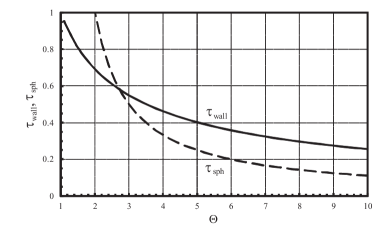
Figure 3: Time limits of the flame acceleration.

Assuming incompressibility for substantially subsonic flame propagation, the continuity equation is given by

$${\frac{{\partial w}}{{\partial\eta}}}+{\frac{{\partial v}}{{\partial\xi}}}=0.$$ (2.1)

The boundary conditions are $v=0$ at the end wall, $\xi=0$, and $w=0$ at the side wall, $\eta=1$. The flow in the fresh mixture (labeled “u”) is assumed to be potential, so Eq. (2.1) yields

$$v_{u}=C_{1}\xi,\qquad w_{u}=C_{1}\left({1-\eta}\right),$$ (2.2)

where the factor $C_{1}$ may depend on time, but is independent of the (radial) coordinate. Recognizing that while the flow in the burnt gas (label “b”) is rotational in general because of the curved flame shape, we can nevertheless treat it as a potential flow close to the end wall, where the flame front is locally planar, see Fig. 2. Subsequently, Eq. (2.1) with the boundary condition at the channel axis, $w=0$ at $\eta=0$, yields the velocity distribution in the burnt gas in the form

$$v_{b}=C_{2}\xi,\qquad w_{b}=-C_{2}\eta.$$ (2.3)

The matching conditions at the flame front, $\eta=\eta_{f}$, are

$${\frac{{d\eta_{f}}}{{d\tau}}}-w_{u}=1,$$ (2.4)

$$v_{u}=v_{b},$$ (2.5)

$$w_{u}-w_{b}=\Theta-1.$$ (2.6)

Here Eq. (2.4) specifies the fixed propagation velocity $S_{L}$ of the flame front with respect to the fuel mixture, while Eqs. (2.5) and (2.6) describe continuity of the tangential velocity at the front and the jump of the normal velocity, respectively. It is noted that the condition (2.5) applies only at the flame skirt close to the wall. Substituting Eqs. (2.2)–(2.3) into Eqs. (2.4)–(2.6), we find $C_{1}=C_{2}=(\Theta-1)$. Consequently,

$$v_{u} = v_{b}=\left(\Theta-1\right)\xi,$$

$$w_{u} = \left(\Theta-1\right)\left(1-\eta\right),$$

$$w_{b} = -\left(\Theta-1\right)\eta,$$ (2.7)

and the evolution equation for the flame skirt, Eq. (2.4), becomes

$$\frac{d\eta_{f}}{d\tau}-(\Theta-1)(1-\eta_{f})=1,$$ (2.8)

which can be integrated with the initial condition $\eta_{f}=0$ at $\tau=0$ as

$$\eta_{f}={\frac{{\Theta}}{{\Theta-1}}}{\left\{{1-\exp{\left[{-\left({\Theta-1}\right)\tau}\right]}}\right\}},$$

$$\tau=-{\frac{{1}}{{\Theta-1}}}\ln\left({1-{\frac{{\Theta-1}}{{\Theta}}}\eta_{f}}\right).$$ (2.9)

According to Eqs. (2.8) and (2.1), we identify two regimes of flame propagation, namely, those with the flame skirt close to the axis and the wall ($\eta_{f}\ll 1$ and $1-\eta_{f}\ll 1$, respectively). In the limit of $\eta_{f}\ll 1$ and $(\Theta-1)\tau\ll 1$, the flame propagates as $d\eta_{f}/d\tau=\Theta$, $\eta_{f}=\Theta\tau$ (i.e. $\dot{R}_{f}=\Theta S_{L}$, $R_{f}=\Theta S_{L}t)$, which is related to the expansion of a semicircular flame front. In the limit of $1-\eta_{f}\ll 1$, a locally planar flame “skirt” approaches the wall, the radial velocity of the fresh fuel mixture tends to zero, and the flame skirt propagates with the planar flame speed with respect to the end wall of the channel, $d\eta_{f}/d\tau=1$ (i.e. $\dot{R}_{f}=S_{L})$. The time of the transition from the hemi-circular to the “finger”-shape flamefront can be estimated as

$$\tau_{sph}\approx{\frac{{1}}{{\Theta-1}}},$$ (2.10)

when the position of the flame skirt, Eq. (2.1), is $\eta_{f,sph}=\left(1-e^{-1}\right)\Theta/\left(\Theta-1\right)\approx 0.63\,\Theta/\left(\Theta-1\right)$ so the transition occurs approximately when the flame skirt has moved more than half-way to the side wall of the channel. Substituting $\eta_{f}=1$ into Eq. (2.10) we find the time when the flame skirt touches the tube wall

$$\tau_{wall}={\frac{{\ln\Theta}}{{\Theta-1}}}.$$ (2.11)

The results (2.10) and (2.11) are shown in Fig. 3 as functions of the expansion factor $\Theta$. It is clearly seen from Eqs. (2.10) and (2.11) and Fig. 3 that the acceleration ($\tau_{sph}<\tau_{wall})$ occurs if $\Theta>e$. For $\Theta=5\sim 10$ we have $\tau_{sph}\approx 0.11\sim 0.25$, while $\tau_{wall}=0.25\sim 0.4$.

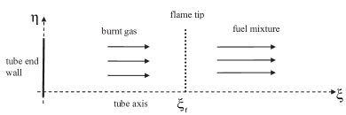
Figure 4: Flow close to the channel axis.

To determine the evolution of the flame tip, we consider the flow along the channel axis, $\eta=0$, as shown in Fig. 4. The flame shape is considered to be locally planar in the vicinity of the centerline ($\eta\rightarrow 0$). In that limit the flow can be considered to be potential, with the longitudinal velocity component $v$ determined by an equation similar to Eq. (2.3). The solution for the longitudinal velocity component $v$ has to coincide with Eq. (2.3) at $\eta\rightarrow 0,\ \xi\rightarrow 0$. Thus, the longitudinal velocity component in the burnt gas $v_{b}$ along the centerline ($\eta=0$) is governed by Eqs. (2.3) and (2.1). We stress that this reasoning does not hold away from the axis in the burnt gas, where the flow is rotational. Still, only the gas velocity along the centerline is utilized in the present analysis. Based on the condition of a fixed propagation velocity of a planar flame front with respect to the burnt gas,

$$\frac{d\xi_{tip}}{d\tau}-v_{b}=\Theta,$$ (2.12)

with $v_{b}$ given by Eq. (2.1), we arrive at the differential equation for the flame tip,

$$\frac{d\xi_{tip}}{d\tau}-(\Theta-1)\xi_{tip}=\Theta,$$ (2.13)

with the initial condition $\xi_{tip}\left(0\right)=0$, and the solution

$$\xi_{tip}={\frac{{\Theta}}{{\Theta-1}}}{\left\{{\exp{\left[{\left({\Theta-1}\right)\tau}\right]}-1}\right\}},$$ (2.14)

which yields a semicircular flame front just after ignition, $(\Theta-1)\tau\ll 1$, when Eq. (2.14) is reduced to $\xi_{tip}=\Theta\tau=\eta_{f}$, and the transition to the exponential acceleration thereafter. According to Eq. (2.14), the growth rate during the exponential stage of acceleration for the planar geometry is given by

$$\sigma_{0,pl}=\Theta-1.$$ (2.15)

At the end of the acceleration, when the flame skirt touches the wall, we have $\tau=\tau_{wall}$, so the position of the flame tip is

$$\xi_{wall}=\xi_{tip}\left(\tau_{wall}\right)=\Theta,$$ (2.16)

or $Z_{wall}=\Theta R$ in dimensional units. Therefore, accounting for Eq. (2.13), we have

$$\left(\frac{d\xi_{tip}}{d\tau}\right)_{wall}=\left(\frac{u_{tip}}{S_{L}}\right)_{max}=\Theta^{2}.$$ (2.17)

To describe the flame shape and evaluate the total increase in the flame surface area during the flame acceleration, we assume, realistically, that at the end of the acceleration the flame shape is almost self-similar, with $\eta_{f}\approx 1$ and $\xi_{tip}\propto\exp{\left[{\left({\Theta-1}\right)\tau}\right]}\gg 1$. We therefore look for the flame shape in the form

$$\xi_{f} = \xi_{tip}(\tau)-f(\tau,\eta),$$

$$f(\tau,\eta) = \varphi\left({\eta}\right)\exp{\left[{\left({\Theta-1}\right)\tau}\right]}.$$ (2.18)

The accuracy of such an approximation is $\Theta^{-1}\ll 1$, which is acceptable for typical flames. Then the equation of flame evolution with respect to the burnt gas can be written as

$${\frac{{\partial f}}{{\partial\tau}}}+w_{b}{\frac{{\partial f}}{{\partial\eta}}}-v_{b}=\Theta{\left[{1+\left({{\frac{{\partial f}}{{\partial\eta}}}}\right)^{2}}\right]}^{1/2}\approx\Theta{\frac{{\partial f}}{{\partial\eta}}}.$$ (2.19)

Accounting for the exponential state of flame acceleration, Eq. (2.1) and the velocity distribution (2.3), we reduce Eq. (2.19) to

$${\left[{\Theta-(\Theta-1)\eta}\right]}{\frac{{d\varphi}}{{d\eta}}}=\Theta,$$ (2.20)

with the boundary condition at the axis, $\varphi\left(0\right)=0$, yielding the solution

$$\varphi\left({\eta}\right)=-{\frac{{\Theta}}{{\Theta-1}}}\ln\left({1-{\frac{{\Theta-1}}{{\Theta}}}\eta}\right),$$ (2.21)

with

$$\xi_{f}\left(\eta,\tau\right)=\frac{\Theta}{\Theta-1}\{\left[{1-\ln\left({1-\frac{\Theta-1}{\Theta}\eta}\right)}\right]\times$$

$$\times\exp{\left[{\left({\Theta-1}\right)\tau}\right]}-1\}.$$ (2.22)

Then the maximum increase in the flame length, achieved when the flame skirt touches the wall, is

$$L_{w}/2R={\int\limits_{0}^{1}{\sqrt{1+\left({{\frac{{\partial f}}{{\partial\eta}}}}\right)^{2}}}}d\eta\approx{\int\limits_{0}^{1}{{\frac{{\partial f}}{{\partial\eta}}}}}d\eta=$$

$$=f(1,\tau_{wall})=\varphi\left({1}\right)\exp{\left[{\left({\Theta-1}\right)\tau_{wall}}\right]}={\frac{{\Theta^{2}\ln\Theta}}{{\Theta-1}}}.$$

2.2 Influence of gas compressibility on acceleration rate for planar geometry

We next consider the problem, with first-order accuracy for the initial flame propagation Mach number $Ma\equiv S_{L}/c_{S,0}\ll 1$, where $c_{S,0}$ is the initial sound speed of the fresh mixture. This approach is conceptually close to that of Refs. Bychkov.et.al-2010a ; Bychkov.et.al-2010b . The compressible counterpart of Eq. (2.12) for the dynamics of the flame tip becomes

$${\frac{{d\xi_{tip}}}{{d\tau}}}-v_{bf}=\vartheta,$$ (2.24)

where $v_{bf}=v_{b}(\xi_{f},\tau)$ is the flow velocity of the burnt gas in the $\xi$-direction just at the flame front, and $\vartheta\equiv\rho_{u}/\rho_{bf}$ the instantaneous gas expansion factor, with $\vartheta_{0}\equiv\Theta$.

As long as $Ma\ll 1$, we can treat the flow ahead of the flame as isentropic. In this case, to first order in $Ma$, we have the following relations for the scaled density $\tilde{\rho}_{u}=\rho_{u}/\rho_{u,0}$, pressure $\tilde{P}_{u}=P_{u}/P_{u,0}$, and temperature $\tilde{T}_{u}=T_{u}/T_{u,0}$ in the fuel mixture

$$\tilde{\rho}_{u} = \left({1+{\frac{{\gamma-1}}{{2}}}{\frac{{v_{u}}}{{c_{S,0}}}}}\right)^{{\frac{{2}}{{\gamma-1}}}}\approx 1+{\frac{{v_{u}}}{{c_{S,0}}}}\approx$$ (2.25)

$$\approx 1+Ma(\Theta-1)\left({\xi{}_{tip}+1}\right),$$

$$\tilde{P}_{u} = \left({1+{\frac{{\gamma-1}}{{2}}}{\frac{{v_{u}}}{{c_{S,0}}}}}\right)^{{\frac{{2\gamma}}{{\gamma-1}}}}\approx 1+\gamma{\frac{{v_{u}}}{{c_{S,0}}}}\approx$$ (2.26)

$$\approx 1+Ma\gamma(\Theta-1)\left({\xi_{tip}+1}\right),$$

$$\tilde{T}_{u} = \left({1+{\frac{{\gamma-1}}{{2}}}{\frac{{v_{u}}}{{c_{S,0}}}}}\right)^{2}\approx 1+(\gamma-1){\frac{{v_{u}}}{{c_{S,0}}}}\approx$$ (2.27)

$$\approx 1+Ma(\gamma-1)(\Theta-1)\left({\xi_{tip}+1}\right),$$

where $\gamma\equiv C_{P}/C_{V}$ is the adiabatic index. It is noted that Eqs. (2.25)–(2.27) also define the rigorous mathematical limit of validity for the present theory, i.e. $v_{u}/c_{S,0}\ll 1$. The matching relations at the flame front are

$$\tilde{\rho}_{u}\left({{\frac{{d\xi_{tip}}}{{d\tau}}}-v_{u}}\right)=\tilde{\rho}_{bf}\left({{\frac{{d\xi_{tip}}}{{d\tau}}}-v_{bf}}\right),$$ (2.28)

$$\tilde{P}_{u}+\tilde{\rho}_{u}\left({{\frac{{d\xi_{tip}}}{{d\tau}}}-v_{u}}\right)^{2}=\tilde{P}_{bf}+\tilde{\rho}_{bf}\left({{\frac{{d\xi_{tip}}}{{d\tau}}}-v_{bf}}\right)^{2},$$ (2.29)

$$\tilde{T}_{u}+\tilde{Q}+{\frac{{1}}{{2C_{P}T_{u,0}}}}\left({{\frac{{d\xi_{tip}}}{{d\tau}}}-v_{u}}\right)^{2}=$$

$$=\tilde{T}_{bf}+{\frac{{1}}{{2C_{P}T_{u,0}}}}\left({{\frac{{d\xi_{tip}}}{{d\tau}}}-v_{bf}}\right)^{2},$$ (2.30)

where $\tilde{Q}\equiv Q/C_{P}T_{u,0}=\Theta-1$ is the scaled reaction heat release. With the first-order approximation for small $Ma$, we reduce Eqs. (2.29) and (2.2) to

$$\tilde{P}_{u}=\tilde{P}_{bf},\ \tilde{T}_{u}+\Theta-1=\tilde{T}_{bf}.$$ (2.31)

Using the perfect gas law, $\tilde{\rho}_{u}\tilde{T}_{u}=\tilde{\rho}_{bf}\tilde{T}_{bf}$, as well as Eq. (2.27), we find

$$\vartheta=1+{\frac{{\Theta-1}}{{\tilde{T}_{u}}}}=\Theta-Ma(\gamma-1)(\Theta-1)^{2}\left({\xi_{tip}+1}\right).$$ (2.32)

While, according to the Euler equation

$${\frac{{\partial v_{b}}}{{\partial\tau}}}+v_{b}{\frac{{\partial v_{b}}}{{\partial\xi}}}=-{\frac{{1}}{{\tilde{\rho}_{b}}}}{\frac{{\partial\tilde{P}_{b}}}{{\partial\xi}}},$$ (2.33)

pressure is uniform in the burnt gas, $\tilde{P}_{b}(\tau)=\tilde{P}_{bf}$, up to the first-order in $Ma\ll 1$, it however grows in time, and thereby increases the temperature and density of the burnt gas due to adiabatic compression.

We next consider propagation of the nearly planar flame “skirt”. Within the accuracy of Ma, the pressure in the fuel mixture between the flame front and the sidewall is the same as that in the burnt gas, $\tilde{P}_{s}=\tilde{P}_{b}(\tau)=\tilde{P}_{bf}=\tilde{P}_{u}$. Thus the density and temperature of the fuel mixture around the flame skirt are the same as those of the fuel mixture just ahead of the flame tip, since in both cases we have adiabatic compression and the same final pressure. Consequently, the continuity equation for the fuel in the domain between the flame shirt and the side wall, $\eta_{f}<\eta<1$, takes the form

$${\frac{{\partial w_{s}}}{{\partial\eta}}}\approx-{\frac{{1}}{{\tilde{\rho}_{s}}}}{\frac{{d\tilde{\rho}_{s}}}{{d\tau}}}=-{\frac{{1}}{{\gamma\tilde{P}_{s}}}}{\frac{{d\tilde{P}_{s}}}{{d\tau}}}=-{\frac{{1}}{{\gamma\tilde{P}_{u}}}}{\frac{{d\tilde{P}_{u}}}{{d\tau}}},$$ (2.34)

with the following solution satisfying the matching relation at the side wall, $\eta=1$, $w_{s}=0$,

$$w_{s} = {\frac{{1}}{{\gamma\tilde{P}_{u}}}}{\frac{{d\tilde{P}_{u}}}{{d\tau}}}\left({1-\eta}\right),$$

$$w_{s,f} = {\frac{{1}}{{\gamma\tilde{P}_{u}}}}{\frac{{d\tilde{P}_{u}}}{{d\tau}}}\left({1-\eta_{f}}\right).$$ (2.35)

Here the subscript “$s,f$” designates the flow velocity just ahead of the flame skirt. Using the matching relations at the flame front, we find the velocity in the burnt gas at the flame skirt, subscripted by “$s,b,f$”, as

$$w_{s,b,f}=w_{s,f}-\vartheta+1={\frac{{1}}{{\gamma\tilde{P}_{u}}}}{\frac{{d\tilde{P}_{u}}}{{d\tau}}}\left({1-\eta_{f}}\right)-\vartheta+1.$$ (2.36)

We subsequently solve the continuity equation, equivalent to Eq. (2.34), in the burnt gas with Eq. (2.36) to find

$$w_{b} = {\frac{{1}}{{\gamma\tilde{P}_{u}}}}{\frac{{d\tilde{P}_{u}}}{{d\tau}}}\left({1-\eta_{f}}\right)-\vartheta+1+{\frac{{1}}{{\gamma\tilde{P}_{u}}}}{\frac{{d\tilde{P}_{u}}}{{d\tau}}}\left({\eta_{f}-\eta}\right)=$$ (2.37)

$$= {\frac{{1}}{{\gamma\tilde{P}_{u}}}}{\frac{{d\tilde{P}_{u}}}{{d\tau}}}\left({1-\eta}\right)-\vartheta+1.$$

Similarly, the continuity equation for the burnt gas around the symmetry axis takes the form

$${\frac{{\partial w_{b}}}{{\partial\eta}}}+{\frac{{\partial v_{b}}}{{\partial\xi}}}=-{\frac{{1}}{{\gamma\tilde{P}_{u}}}}{\frac{{d\tilde{P}_{u}}}{{d\tau}}},$$ (2.38)

which can be integrated as

$$v_{b}=\left({\vartheta-1}\right)\xi-{\frac{{1}}{{\gamma\tilde{P}_{u}}}}{\frac{{d\tilde{P}_{u}}}{{d\tau}}}\xi,\qquad w_{b}=-\left({\vartheta-1}\right)\eta.$$ (2.39)

Consequently, the evolution equation for the flame tip, Eq. (2.24), becomes

$${\frac{{d\xi_{tip}}}{{d\tau}}}=\left({\vartheta-1-{\frac{{1}}{{\gamma\tilde{P}_{u}}}}{\frac{{d\tilde{P}_{u}}}{{d\tau}}}}\right)\xi_{tip}+\vartheta.$$ (2.40)

Finally, substituting Eqs. (2.26) and (2.32) into Eq. (2.40), neglecting the second- and higher-order terms in $Ma$, and accounting for the zeroth-order approximation, Eq. (2.14), we obtain

$${\frac{{d\xi_{tip}}}{{d\tau}}}=-Ma\gamma\left({\Theta-1}\right)^{2}\xi_{tip}^{2}+\sigma_{1,pl}\xi_{tip}+\Theta_{1},$$ (2.41)

with

$$\sigma_{1,pl}=\left({\Theta-1}\right){\left[{1-Ma\left({\Theta+2\left({\gamma-1}\right)\left({\Theta-1}\right)}\right)}\right]},$$ (2.42)

$$\Theta_{1}=\Theta-Ma(\gamma-1)(\Theta-1)^{2}.$$ (2.43)

In the limit of incompressible flow, $Ma=0$, we have $\sigma_{1,pl}=\Theta-1$, $\Theta_{1}=\Theta$, and Eq. (2.41) fully reproduces Eq. (2.13). Accounting for gas compressibility, we obtain moderation of the flame acceleration in Eq. (2.41), which is described by two types of terms: linear and nonlinear with respect to $\xi_{tip}$. The linear term does not change the exponential state of the flame acceleration, though they reduce the acceleration rate to $\sigma_{1,pl}$ as compared to $\Theta-1$ for the incompressible flow. At the very beginning, for $\xi_{tip}\to 0$, the flame acceleration is moderated by the linear terms only, and Eq. (2.41) reduces to

$$\frac{d\xi_{tip}}{d\tau}=\sigma_{1,pl}\xi_{tip}+\Theta_{1},$$ (2.44)

with the solution

$$\xi_{tip}={\frac{{\Theta_{1}}}{{\sigma_{1,pl}}}}{\left[{\exp\left({\sigma_{1,pl}\tau}\right)-1}\right]}.$$ (2.45)

The nonlinear term of Eq. (2.41), however, becomes important quite fast and modifies the exponential state of flame acceleration to a slower one. The complete analytical solution to Eq. (2.41) is given by

$$\xi_{tip}={\frac{{2\Theta_{1}\,{\left[{\exp\left({\sigma_{2}\tau}\right)-1}\right]}}}{{\left({\sigma_{2}-\sigma_{1,pl}}\right)\exp\left({\sigma_{2}\tau}\right)+\left({\sigma_{2}+\sigma_{1,pl}}\right)}}},$$ (2.46)

where $\sigma_{2}\equiv\sqrt{\sigma_{1,pl}^{2}+4Ma\gamma\Theta_{1}\left(\Theta-1\right)^{2}}$.

2.3 Influence of gas compressibility for the axi-symmetric geometry

Now we reconsider the problem in an axi-symmetric, cylindrical tube, Ref. Bychkov.et.al-2007 , incorporating compressibility with the accuracy of the first order for flame propagation Mach number.

The incompressible continuity equation in the axi-symmetric geometry takes the form Bychkov.et.al-2007

$$\frac{1}{\eta}\frac{\partial}{\partial\eta}\left(\eta w\right)+\frac{\partial v}{\partial\xi}=0,$$ (2.47)

and the axi-symmetric counterparts for the velocity distributions, Eq. (2.1), and the evolution of the flame skirt, Eqs. (2.8)–(2.1), are given by

$$v_{u} = v_{b}=2\left(\Theta-1\right)\eta_{f}\xi,$$

$$w_{u} = \left(\Theta-1\right)\eta_{f}\left(\frac{1}{\eta}-\eta\right),$$

$$w_{b} = -\left(\Theta-1\right)\eta_{f}\eta,$$ (2.48)

$$\frac{d\eta_{f}}{d\tau}-(\Theta-1)(1-\eta_{f}^{2})=1\qquad\Longrightarrow$$ (2.49)

$$\eta_{f} = \frac{\Theta}{\alpha}\tanh\left(\alpha\tau\right),$$

$$\tau_{wall} = \frac{1}{2\alpha}\ln\left(\frac{\Theta+\alpha}{\Theta-\alpha}\right),$$

$$\tau_{sph} = \frac{1}{2\alpha},$$ (2.50)

where

$$\alpha=\sqrt{\Theta\left(\Theta-1\right)}.$$ (2.51)

It can be readily shown from Eq. (2.3) that acceleration is possible (i.e. $\tau_{sph}<\tau_{wall}$) if $\Theta>\left({1-[(e-1)/e+1)]^{2}}\right)^{-1}\approx 1.27$. For $\Theta=5\sim 10$, Eq. (2.3) yields $\tau_{sph}\approx 0.05\sim 0.11$, and $\tau_{wall}\approx 0.19\sim 0.32$. These quantities are much smaller than those of the planar geometry, Eqs. (2.10) and (2.11), making an indirect proof that for the axisymmetric geometry acceleration proceeds faster than the planar one.

With the result (2.3), equation for the flame tip, $\dot{\xi_{tip}}-v_{b}=\Theta$, becomes

$$\frac{d\xi_{tip}}{d\tau}-2(\Theta-1)\eta_{f}(\tau)\xi_{tip}(\tau)=\Theta,$$ (2.52)

or

$$\frac{d\xi_{tip}}{d\tau}-2\alpha\tanh\left(\alpha\tau\right)\xi_{tip}=\Theta,$$ (2.53)

with the solution

$$\xi_{tip}=\frac{\Theta}{2\alpha}\sinh\left(2\alpha\tau\right),$$ (2.54)

which also yields $\xi_{wall}=\Theta$ similar to the 2D result (2.16). At sufficiently late times we have $\eta_{f}\approx 1$ and Eqs. (2.52)–(2.53) reduce to

$$\frac{d\xi_{tip}}{d\tau}=2\alpha\xi_{tip}+\Theta\qquad\Longrightarrow$$

$$\qquad\xi_{tip}=\frac{\Theta}{2\alpha}\left[\exp\left(2\alpha\tau\right)-1\right],$$ (2.55)

so the flame tip accelerates almost exponentially, with the acceleration rate

$$\sigma_{0,axi}=2\alpha=2\sqrt{\Theta(\Theta-1)}.$$ (2.56)

This result exceeds considerably (by a factor of about 2) its 2D counterpart ($\Theta-1$), see Eq. (2.15), and it is slightly smaller than the model estimation $2\Theta$ of Clanet and Searby Clanet.Searby-1996 .

Now we account for small, but finite gas compression. With the axial velocity $v_{u}$ given by Eq. (2.3), the axi-symmetric counterparts of Eqs. (2.25)–(2.27) and (2.32) are

$$\tilde{\rho}_{u} = \left(1+\frac{\gamma-1}{2}\frac{v_{u}}{c_{0}}\right)^{\frac{2}{\gamma-1}}\approx$$ (2.57)

$$\approx 1+Ma\left(2\alpha\xi_{tip}+\Theta-1\right),$$

$$\tilde{P}_{u} = \left(1+\frac{\gamma-1}{2}\frac{v_{u}}{c_{0}}\right)^{\frac{2\gamma}{\gamma-1}}\approx$$ (2.58)

$$\approx 1+Ma\gamma\left(2\alpha\xi_{tip}+\Theta-1\right),$$

$$\tilde{T}_{u} = \left(1+\frac{\gamma-1}{2}\frac{v_{u}}{c_{0}}\right)^{2}\approx$$ (2.59)

$$\approx 1+Ma\left(\gamma-1\right)\left(2\alpha\xi_{tip}+\Theta-1\right),$$

$$\vartheta=\Theta-Ma(\gamma-1)(\Theta-1)^{2}\left(2\frac{\Theta}{\alpha}\xi_{tip}+1\right).$$ (2.60)

Following the strategy of Section 2.2, we find

$${\frac{{1}}{{\eta}}}{\frac{{\partial}}{{\partial\eta}}}\left({\eta w_{b}}\right)+{\frac{{\partial v_{b}}}{{\partial\xi}}}=-{\frac{{1}}{{\gamma\tilde{P}_{u}}}}\frac{{d\tilde{P}_{u}}}{{d\tau}}\qquad\Longrightarrow\qquad$$ (2.61)

$$v_{b} = 2\left({\vartheta-1}\right)\eta_{f}\xi-{\frac{{1}}{{\gamma\tilde{P}_{u}}}}{\frac{{d\tilde{P}_{u}}}{{d\tau}}}\xi{\rm,}$$

$$w_{b} = -\left({\vartheta-1}\right)\eta_{f}\eta.$$ (2.62)

Similar to Eqs. (2.49) and (2.3), the flame skirt position is given by

$$\frac{d\eta_{f}}{d\tau}-(\vartheta-1)(1-\eta_{f}^{2})=1\qquad\Longrightarrow\qquad\eta_{f}=\frac{\vartheta}{\hat{\alpha}}\tanh\left(\hat{\alpha}\tau\right),$$ (2.63)

where $\hat{\alpha}=\sqrt{\vartheta\left(\vartheta-1\right)}$, and the evolution equation for the flame tip is

$${\frac{{d\xi_{tip}}}{{d\tau}}}=\left({2\left({\vartheta-1}\right)\eta_{f}-{\frac{{1}}{{\gamma\tilde{P}_{u}}}}{\frac{{d\tilde{P}_{u}}}{{d\tau}}}}\right)\xi_{tip}+\vartheta.$$ (2.64)

Holding the zeroth- and first-order approximations for $Ma$ in Eq. (2.64), we rewrite it in the form

$$\frac{d\xi_{tip}}{d\tau}=\left[2\hat{\alpha}\tanh\left(\hat{\alpha}\tau\right)-2Ma\vartheta\alpha\right]\xi_{tip}-$$

$$-4Ma\alpha\hat{\alpha}\tanh\left(\hat{\alpha}\tau\right)\xi_{tip}^{2}+\vartheta,$$ (2.65)

or

$$\frac{d\xi_{tip}}{d\tau}=\left\{2\alpha_{1}\tanh\left(\alpha_{1}\tau\right)-2Ma\,\alpha\left[1+\gamma\left(\Theta-1\right)\right]\right\}\xi_{tip}-$$

$$-2Ma\left\{\frac{\alpha\tau B}{\cosh^{2}\left(\alpha\tau\right)}+\left(2\alpha^{2}-B\right)\tanh\left(\alpha\tau\right)\right\}\xi^{2}_{tip}+\Theta_{1}$$

where $\Theta_{1}$ is the same as in the planar geometry, see Eq. (2.43), and

$$\alpha_{1} = \sqrt{\Theta_{1}\left(\Theta_{1}-1\right)},$$

$$B = \left(\gamma-1\right)\left(\Theta-1\right)\left(2\Theta-1\right).$$ (2.67)

In general, Eq. (2.3) has to be solved computationally, but we shall integrate it analytically with several asymptotic approaches. First, in the limit of $Ma=0$, we have $\Theta_{1}=\Theta$, $\alpha_{1}=\alpha$ and Eq. (2.3) reproduces Eq. (2.53). Even for finite gas compressibility, the effect of the nonlinear term in Eq. (2.3) is negligible in the very beginning, hence Eq. (2.3) can be approximated by

$$\frac{d\xi_{tip}}{d\tau} = \{2\alpha_{1}\tanh\left(\alpha_{1}\tau\right)-$$ (2.68)

$$- 2Ma\,\alpha\left[1+\gamma\left(\Theta-1\right)\right]\}\xi_{tip}+\Theta_{1},$$

with the solution to the first-order approximation for $Ma$ being

$$\xi_{tip} = \frac{\Theta_{1}}{2\alpha_{1}}\sinh\left(2\alpha_{1}\tau\right)-$$

$$- 2Ma\frac{\Theta}{\alpha}\left[1+\gamma\left(\Theta-1\right)\right]\cosh^{2}\left(\alpha\tau\right)\ln\cosh\left(\alpha\tau\right).$$

The nonlinear term of Eq. (2.3), however, becomes important quite fast, modifying the state of flame acceleration to a slower one, and hence making the asymptote (2.3) incorrect. However, at a sufficiently late stage of the acceleration, we can approximate $\tanh\left(\alpha_{1}\tau\right)\sim 1$, hence $\eta_{f}\sim\vartheta/\hat{\alpha}$, and Eq. (2.3) is reduced to a form similar to that of the 2D, Eq. (2.41) ,

$${\frac{{d\xi_{tip}}}{{d\tau}}}=-Ma\psi\xi_{tip}^{2}+\sigma_{1,axi}\xi_{tip}+\Theta_{1},$$ (2.70)

where

$$\psi=2\left({\Theta-1}\right)\left(2\Theta\gamma-\gamma+1\right),$$ (2.71)

$$\sigma_{1,axi}=\sigma_{0,axi}{\left\{{1-Ma{\left[{\Theta+\frac{4\Theta-1}{2\Theta}\left({\gamma-1}\right)\left({\Theta-1}\right)}\right]}}\right\}},$$ (2.72)

and with the solution, Eq. (2.46),

$$\xi_{tip}={\frac{{2\Theta_{1}{\left[{\exp\left({\sigma_{2}\tau}\right)-1}\right]}}}{{\left({\sigma_{2}-\sigma_{1,axi}}\right)\exp\left({\sigma_{2}\tau}\right)+\left({\sigma_{2}+\sigma_{1,axi}}\right)}}},$$ (2.73)

where $\sigma_{2}\equiv\sqrt{\sigma_{1,axi}^{2}+4\Theta_{1}Ma\psi}$ in the axisymmetric configuration. Obviously, the result (2.70) to (2.73) fully recovers the properties of its planar counterpart: in the limit of $Ma=0$ we have $\sigma_{1,axi}=\sigma_{0,axi}$, and Eqs. (2.70) and (2.73) reduce to Eq. (2.3); accounting for gas compressibility, we obtain linear and nonlinear moderation of the flame acceleration with respect to $\xi_{tip}$. Reducing the acceleration rate from $\sigma_{0,axi}$ to $\sigma_{1,axi}$, the linear terms do not change the exponential state of acceleration while the nonlinear term of Eq. (2.70) modifies the exponential state of flame acceleration to a slower one as soon as it becomes important.

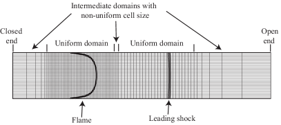
Figure 5: The sketch of the grid with variable resolution used in numerical simulations.

It is emphasized that the result (2.73) does not reproduce the asymptote (2.3) as they are related to opposite limiting cases. Consequently, it is expected that for a certain range of $Ma$ the complete (numerical) solution to Eq. (2.3) lies in between the two values given by Eqs. (2.3) and (2.73).

3 Numerical method, basic equations, boundary and initial conditions

We perform numerical simulations of the hydrodynamic and combustion equations including transport processes (thermal conduction, diffusion, viscosity) and chemical kinetics in the form of Arrhenius equation. Both 2D planar and axisymmetric cylindrical flows are investigated. In the general tensor form the governing equations are given by

$${\frac{{\partial\rho}}{{\partial t}}}+{\frac{{1}}{{r^{\beta}}}}{\frac{{\partial}}{{\partial r}}}\left({r^{\beta}\rho u_{r}}\right)+{\frac{{\partial}}{{\partial z}}}\left({\rho u_{z}}\right)=0,$$ (3.1)

$$\frac{\partial}{\partial t}\left(\rho u_{r}\right) + \frac{1}{r^{\beta}}\frac{\partial}{\partial r}{\left[{r^{\beta}\left({\rho u_{r}^{2}-\zeta_{r,r}}\right)}\right]}+$$

$$+ {\frac{{\partial}}{{\partial z}}}\left({\rho u_{r}u_{z}-\zeta_{r,z}}\right)+{\frac{{\partial P}}{{\partial r}}}+\psi_{\beta}=0,$$

$${\frac{{\partial}}{{\partial t}}}\left({\rho u_{z}}\right) + {\frac{{1}}{{r^{\beta}}}}{\frac{{\partial}}{{\partial r}}}{\left[{r^{\beta}\left({\rho u_{r}u_{z}-\zeta_{r,z}}\right)}\right]}+$$ (3.3)

$$+ {\frac{{\partial}}{{\partial z}}}\left({\rho u_{z}^{2}-\zeta_{z,z}}\right)+{\frac{{\partial P}}{{\partial z}}}=0{\rm,}$$

$${\frac{{\partial\varepsilon}}{{\partial t}}} + {\frac{{1}}{{r^{\beta}}}}{\frac{{\partial}}{{\partial r}}}{\left[{r^{\beta}\left({\left({\varepsilon+P}\right)u_{r}-\zeta_{r,r}u_{r}-\zeta_{r,z}u_{z}+q_{r}}\right)}\right]}+$$ (3.4)

$$+ {\frac{{\partial}}{{\partial z}}}{\left[{\left({\varepsilon+P}\right)u_{z}-\zeta_{z,z}u_{z}-\zeta_{r,z}u_{r}+q_{z}}\right]}=0,$$

$$\frac{\partial}{\partial t}\left({\rho Y}\right) + \frac{1}{r^{\gamma}}\frac{\partial}{\partial r}{\left[{r^{\gamma}\left({\rho u_{i}Y-\frac{\mu}{Sc}\frac{\partial Y}{\partial r}}\right)}\right]}+$$ (3.5)

$$+ \frac{\partial}{\partial z}\left(\rho u_{z}Y-\frac{\mu}{Sc}\frac{\partial Y}{\partial z}\right)=$$

$$= -\frac{\rho Y}{\tau_{R}}\exp\left(-E_{a}/\overline{R}T\right),$$

where $\beta=0$ and 1 for 2D and axisymmetric geometries, respectively,

$$\varepsilon=\rho\left({QY+C_{V}T}\right)+{\frac{{\rho}}{{2}}}\left({u_{z}^{2}+u_{r}^{2}}\right)$$ (3.6)

is the total energy per unit volume, $Y$ the mass fraction of the fuel, $Q$ the energy release from the reaction, and $C_{V}$ the heat capacity at constant volume. The energy diffusion vector $q_{i}$ is given by

$$q_{r}=-\mu\left({{\frac{{C_{P}}}{{Pr}}}{\frac{\partial T}{\partial r}}+\frac{Q}{Sc}{\frac{\partial Y}{\partial r}}}\right),$$ (3.7)

$$q_{z}=-\mu\left({{\frac{{C_{P}}}{{Pr}}}{\frac{{\partial T}}{{\partial z}}}+{\frac{Q}{Sc}}{\frac{\partial Y}{\partial z}}}\right).$$ (3.8)

In the 2D configuration ($\beta=0)$ the stress tensor $\zeta_{i,j}$ takes the form

$$\zeta_{i,j}=\mu\left({{\frac{{\partial u_{i}}}{{\partial x_{j}}}}+{\frac{{\partial u_{j}}}{{\partial x_{i}}}}-{\frac{{2}}{{3}}}{\frac{{\partial u_{k}}}{{\partial x_{k}}}}\delta_{i,j}}\right),$$ (3.9)

while in the axisymmetric geometry ($\beta=1)$ it reads

$$\zeta_{r,r}={\frac{{2\mu}}{{3}}}\left({2{\frac{{\partial u_{r}}}{{\partial r}}}-{\frac{{\partial u_{z}}}{{\partial z}}}-{\frac{{u_{r}}}{{r}}}}\right),$$ (3.10)

$$\zeta_{z,z}={\frac{{2\mu}}{{3}}}\left({2{\frac{{\partial u_{z}}}{{\partial z}}}-{\frac{{\partial u_{r}}}{{\partial r}}}-{\frac{{u_{r}}}{{r}}}}\right),$$ (3.11)

$$\zeta_{r,z}=\mu\left({{\frac{{\partial u_{r}}}{{\partial z}}}+{\frac{{\partial u_{z}}}{{\partial r}}}}\right).$$ (3.12)

Finally, the last term in Eq. (3) takes the form

$$\psi_{\beta}={\frac{{2\mu}}{{3}}}\left({2{\frac{{u_{r}}}{{r}}}-{\frac{{\partial u_{r}}}{{\partial r}}}-{\frac{{\partial u_{z}}}{{\partial z}}}}\right)$$ (3.13)

if $\beta=1$, and $\psi_{\beta}=0$ if $\beta=0$. Here $\mu$ is the dynamic viscosity, and $Pr$ and $Sc$ the Prandtl and Schmidt numbers, respectively.

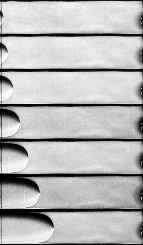
Figure 6: Schlieren images of finger flame propagation for stoichiometric $H_{2}/O_{2}$ mixture at pressure 0.2 bar. The shown images are evenly distributed in time with interval of 100 ms. Note that the shift of image’s left boundary is 10 mm to the right as compared to the position of the end wall and ignition point.

We take unity Lewis number $Le\equiv Sc/Pr=1$, with $Pr=Sc=0.75$; the dynamical viscosity is $\mu=1.7\times 10^{-5}\,{\rm N}{\rm s}{\rm/}{\rm m}^{{\rm 2}}$. The fuel-air mixture and burnt gas are perfect gases with a constant molar mass $m=2.9\times 10^{-2}{\rm kg}/{\rm mol}$, with $C_{V}=5\overline{R}/2m$, $C_{P}=7\overline{R}/2m$, and the equation of state

$$P=\rho\overline{R}T/m,$$ (3.14)

where $\overline{R}\approx 8.31\,\mathrm{J}/(\mathrm{mol}\cdot\mathrm{K})$ is the universal gas constant. We consider a single-step irreversible reaction of the first order with the temperature dependence of the reaction rate given by the Arrhenius law with an activation energy $E_{a}$ and the factor of time dimension $\tau_{R}$. In our simulations we took $E_{a}/\overline{R}T_{u}=32$ in order to have better resolution of the reaction zone. The factor $\tau_{R}$ was adjusted to obtain a particular value of the planar flame velocity $S_{L}$ by solving the associated eigenvalue problem. The flame thickness is defined as

$$L_{f}\equiv{\frac{{\mu_{u}}}{{\Pr\rho_{u}S_{L}}}},$$ (3.15)

where $\rho_{u}=1.16\,\rm{kg/m^{3}}$ is the unburned mixture density. It is noted that $L_{f}$ is just a mathematical parameter of length dimension related to the flame front, while the real effective diffusion flame thickness is considerably larger Poinsot.Veynante-2001 ; Akkerman.et.al-2006-2 . We took initial temperature of the fuel mixture $T_{u,0}=300K$, initial pressure $P_{u,0}=10^{5}\ Pa$, specific heat ratio $\gamma=1.4$, and $\Theta=8$. We performed the simulations for a rather wide range of initial Mach number $Ma=S_{L}/c_{S,0}=10^{-3}\sim 1.6\times 10^{-2}$, with the lower and upper values being relevant to hydrocarbon and hydrogen-oxygen flames, respectively Kuznetsov.et.al-2005 . We used the tube diameter $2R=150L_{f}$ and channel width $2R=100L_{f}$ for axisymmetric and 2D simulations, respectively.

Similar to the theoretical analysis, we adopt slip and adiabatic boundary conditions at the tube walls:

$${\rm{\bf n}}\cdot{\rm{\bf u}}=0,\quad{\rm{\bf n}}\cdot\nabla T=0,$$ (3.16)

where ${\rm{\bf n}}$ is the unit normal vector at the walls. At the open face end of the tube/channel non-reflecting boundary conditions are applied. As initial conditions, we used a semi-circular flame “ignited” at the channel axis at the closed end of the tube, with its structure given by the analytical solution of Zel’dovich and Frank-Kamenetskii Zeldovich.et.al.-1985 ; Law-2006

$$T=T_{u}+(T_{b}-T_{u})\exp\left({-\sqrt{x^{2}+z^{2}}/L_{f}}\right),$$

$$\textrm{if}\ z^{2}+x^{2}<r_{f}^{2}$$ (3.17)

$$T=\Theta T_{u},\ \textrm{if}\ z^{2}+x^{2}>r_{f}^{2}$$ (3.18)

$$Y=(T_{b}-T)/(T_{b}-T_{f}),\quad P=P_{u},$$

$$u_{x}=0,\quad u_{z}=0.$$ (3.19)

Here $r_{f}$ is the radius of the initial flame ball at the closed end of the tube. The finite initial radius of the flame ball is equivalent to a time shift, which requires proper adjustments when comparing the theory and numerical simulations.

The simulations used a 2D hydrodynamic Navier-Stokes code adapted for parallel computations Wollblad.et.al-2006 . The numerical scheme is second order accurate in time and fourth order accurate in space for convective terms, and second order in space for diffusive terms. The code is robust and accurate; it was successfully used in aero-acoustic applications. 2D and axisymmetric simulations were conducted. We used mesh with variable resolution in order to take into account the growing distances between the tube end, the accelerating flame and the pressure wave, and to resolve both chemical and hydrodynamic spatial scales. Typical computation time for one simulation required up to $10^{4}$ CPU-hours, hence implying the need for extensive parallel calculations.

A rectangular grid with the grid walls parallel to the coordinate axes was used. The sketch of the calculation mesh used in simulations of flame acceleration from the closed tube end is shown in Fig. 5. To perform all the calculations in a reasonable time, we made the grid spacing non-uniform along the $z$-axis with the zones of fine grid around the flame and leading shock fronts. For majority of the simulation runs, the grid size in the $z$-direction was 0.25$L_{f}$ and 0.5$L_{f}$ in the domains of the flame and leading pressure wave, respectively, which allowed resolution of the flame and waves. Outside the region of fine grid the mesh size increased gradually with 2% change in size between the neighboring cells. In order to keep the flame and pressure waves in the zone of fine grid we implemented the periodical mesh reconstruction during the simulation run Valiev.et.al-2008 . Third-order splines were used for the re-interpolation of the flow variables during periodic grid reconstruction to preserve the second order accuracy of the numerical scheme.

4 Results and discussion

4.1 Experimental results

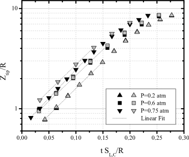
Figure 7: Scaled flame tip position versus scaled time for different pressures: $P=0.2\ \textrm{bar}$ (triangles), $P=0.6\ \textrm{bar}$ (squares), $P=0.75\ \textrm{bar}$ (upside down triangles). Different color for each pressure correspond to different experimental runs.

Experiments were performed in a channel with rectangular cross-section (50 $\times$ 50 mm), 6.05 m long with 24 transparent ports for photo-gauges. A high-speed schlieren system with stroboscopic pulse generator and high speed camera, germanium photodiodes and piezoelectric transducers were used to record the flame evolution. The experimental facilities, including ignition conditions, are described in detail in Ref. Kuznetsov.et.al-2005 ; Kuznetsov.et.al-2010 and the references given therein.

$P$, bar	$\Theta$	$L_{T}$, mm	$C$	$S_{L}$, m/s	$S_{L,C}$, m/s	$Ma$	$Ma_{C}$	$\sigma_{1}$	$\sigma_{1,C}$
0.20	8.00	2.0	0.778	6.855	5.33	0.0128	0.0100	4.18	5.373
0.60	8.260	0.5	0.944	8.395	7.928	0.0157	0.0149	4.83	5.138
0.75	8.317	0.379	0.958	8.700	8.335	0.0162	0.0157	4.90	5.110
0.75	8.317	0.379	0.958	8.700	8.335	0.0162	0.0157	5.43	5.660

Table 1: Experiment parameters and $\sigma_{1,C}$ obtained by fitting of the results of Fig. 7 for different pressures.

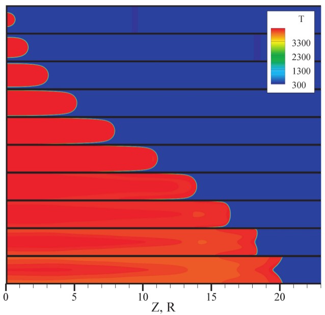
Figure 8: Temperature field evolution and “tulip” formation for planar geometry, $\Theta=14$, and Mach number $Ma=0.005$ at different time instants. Time instants are equally spaced in the range of $(0.04022\div 0.42161)S_{L}t/R$.

The experiments were conducted with the fast-burning, stoichiometric hydrogen–oxygen mixture at initial pressures of $0.2\sim 0.75$ bar. The mixture was prepared by precise partial pressure method with deviation less than $\pm 0.2\%$ with respect to the $H_{2}$ fraction. By changing the initial pressure we vary the value of $S_{L}$ and the initial flame Mach number. The initial ambient gas mixture temperature was $T_{0}=293K$; and the corresponding sound speed is 531 m/s. The initial density ratio is in the range $\Theta=8.0\sim 8.317$, depending on the initial pressure. It is noted that for such highly reactive fuel mixtures the influence of the ignition source on the initial flame dynamics is negligible, as compared with the influence of mixture reactivity, expansion ratio and tube diameter. The ignition energy of 2-10 mJ is about $10^{3}$ times lower than the released combustion energy at the initial stage of finger flame propagation (with the diameter of flame ball smaller than 1 cm).

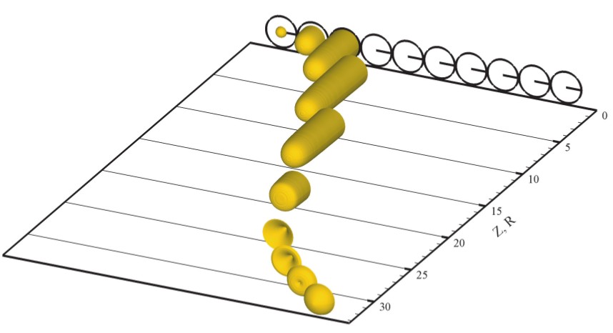
Figure 9: Flame shape evolution and “tulip” formation for axisymmetric geometry, $\Theta=14$, and Mach number $Ma=0.005$ at different time instants. Time instants are equally spaced in the range of $(0.02692\div 0.26576)S_{L}t/R$. Isosurfaces are shown for $T=1400K$.

Figure 6 shows the schlieren images of “finger” flame propagation at a pressure of 0.2 bar. It is seen that the flame tip accelerates exponentially at the initial stage of flame propagation, in agreement with previous experiments Clanet.Searby-1996 and theory Bychkov.et.al-2007 . For the stoichiometric $H_{2}/O_{2}$ fuel mixture used in the present experiment the influences of diffusional-thermal cellular and pulsating instabilities Law-2006 are ruled out. The influence of hydrodynamic (Darrieus-Landau) instability is negligible as well due to the strong flame curvature observed in the experiment, leading to the Zeldovich-type stabilization of the flame front perturbations Liberman.et.al-2003 . Moreover, even if the Darrieus-Landau instability is developed, its scaled exponential acceleration rate would be about unity Zeldovich.et.al.-1985 ; Law-2006 , which is up to an order of magnitude smaller than the finger flame acceleration rate of Eqs. (2.15), (2.42), (2.56), (2.72), thereby diminishing any possible role of the DL instability as compared to the finger-flame acceleration effects. Consequently, in the present experiment the flame front acceleration could be attributed purely to the finger-flame mechanism of exponential acceleration Clanet.Searby-1996 ; Bychkov.et.al-2007 .

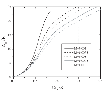
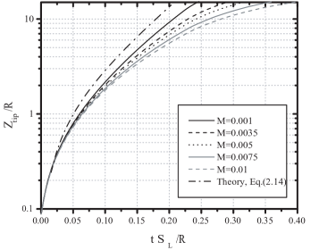
Figure 10: Scaled flame tip position versus time for planar geometry, $\Theta=14$, and Mach numbers $Ma=0.001,\ 0.0035,\ 0.005,\ 0.0075,\ 0.01$: (a) linear scale, (b) logarithmic scale.

The experimentally obtained evolution of the scaled flame tip position for various pressures is shown in Fig. 7. The definition of the laminar burned velocity $S_{L,C}$ used in the present scaling is described further. When the flame skirt approaches the wall, the flame acceleration weakens, and the flame shape undergoes transition from a convex “finger” to a concave “tulip” shape. The instant when the flame skirt approaches the channel wall is clearly correlated with the instant at which the exponential flame tip acceleration terminates, which can be seen at Fig. 7.

Figure 11: Scaled velocity of flame tip versus time for planar geometry, $\Theta=14$, and Mach numbers $Ma=0.001,\ 0.0035,\ 0.005,\ 0.0075,\ 0.01$.

Physical parameters of the experiments, as well as the scaled acceleration rates obtained from fitting of experimental results of Fig. 7 for different pressures, and the initial Mach numbers are given in Table 1. The unstretched laminar flame velocity $S_{L}$ and the thermal flame thickness $L_{T}$ are obtained from the numerical simulation of one-dimensional premixed flame structure employing PREMIX code of the CHEMKIN family Kee-2000 with the use of updated chemical kinetics mechanism for hydrogen oxidation Burke-2011 . The thermal flame thickness $L_{T}$ is conventionally defined as Law-2006 $(T_{b}-T_{u})/\max(|\partial T/\partial x|)$, where $T_{b}$ and $T_{u}$ are the temperatures of burnt and unburnt gases, respectively, and $\max(|\partial T/\partial x|)$ is the maximum of the temperature gradient. It is noted that in our case of low-pressure stoichiometric hydrogen-oxygen finger flames a noticeable pure curvature effect Law-2006 is observed, therefore we introduce relevant modifications to $S_{L}$ and $Ma$, denoted as $S_{L,C}$ and $Ma_{C}$, in such a mannner that the correction parameter $C$ is defined as $C=S_{L,C}/S_{L}$, so that the estimation for the modified growth rate is given by $\sigma_{1,C}=\sigma_{1}/C$. It is seen that, the lower is the pressure, the larger is the thermal flame thickness, and consequently the more pronounced is the pure curvature effect.

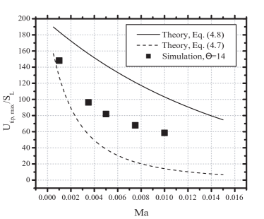
Figure 12: Scaled maximum flame tip velocity versus Mach number obtained in simulations for planar geometry, $\Theta=14$, is compared to theoretical estimates. Solid line - Eq. (4.8), dashed line - Eq. (4.7)

The pure curvature correction parameter $C$ and the modified growth rate $\sigma_{1,C}$ are estimated as follows. Based on experimental observation, we assume, realistically, that the curvature of the flame tip remains almost constant during the time interval $\tau_{sph}<\tau<\tau_{wall}$, with $\tau_{sph}$ and $\tau_{wall}$ given by Eqs. (2.10) and (2.11), respectively. Within this time the flame tip radius can be approximated as

$$R_{tip}=R\eta_{f,sph}=0.63\,R\Theta/\left(\Theta-1\right)\approx 0.72R,$$ (4.1)

where $R$ is the channel half-width. Consequently, with the curvature term in the form $\nabla\cdot\mathbf{n}=2/R_{tip}$, the curvature-modified laminar burning velocity at the flame tip can be estimated as Law-2006

$$S_{L,C}=CS_{L}=S_{L}\left(1-L_{T}\nabla\cdot\mathbf{n}\right)=S_{L}\left(1-\frac{2L_{T}}{R_{tip}}\right).$$ (4.2)

As Table 1 shows, modified values of the growth rate $\sigma_{1,C}$ decrease with increasing $Ma$, while the uncorrected growth rate $\sigma_{1}$ increases instead. This demonstrates a non-negligible effect of pure curvature for low-pressure $H_{2}/O_{2}$ finger flames, disregarding which could reverse the main trend. For this reason, an accurate determination of the laminar burning velocity is crucial for the analysis of experimental results. This is particularly relevant for the extraction of the growth rate $\sigma_{1}$ for various $Ma$, since even a 15-20% difference in the laminar burning velocity could lead to a completely erroneous conclusion.

4.2 Numerical results and discussion

We performed numerical simulation of the flame acceleration in tubes with smooth slip adiabatic walls at different flow parameters. Particularly, we employed planar and axisymmetric geometries, and a range of initial flame propagation Mach numbers $Ma=10^{-3}\sim 1.6\times 10^{-2}$. We also used two values of the thermal expansion ratio $\Theta=8,\ 14$.

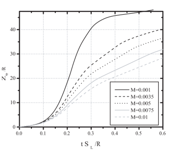
Figure 13: Scaled flame tip position versus time for axisymmetric geometry, $\Theta=14$, and Mach numbers $Ma=0.001,\ 0.0035,\ 0.005,\ 0.0075,\ 0.01$: (a) linear scale, (b) logarithmic scale.

We illustrate evolution of the temperature field for the planar geometry in Fig. 8 for $\Theta=14$ and the initial Mach number $Ma=0.005$. The simulation plots also show the instant of transition from a convex “finger” to a concave “tulip” flame shape. It is seen that, similar to the experimental Figure 6, the flame tip curvature does not change significantly from the instant of the transition to the finger configuration and until the flame skirt touches the wall, thus justifying the assumption of almost constant tip curvature made in Sec. 4.1. It should be noted that formation of finger-shaped laminar flame fronts in planar geometry due to essentially different Schelkin mechanism has been also obtained in simulations of premixed flames in channels with non-slip walls Kagan-2003 ; Valiev.et.al-2008 ; Valiev.et.al-2009 . Furthermore similar shapes of the finger front were observed within the context of electrochemical doping in organic semiconductors Bychkov.et.al-2011 ; Bychkov.et.al-2012 , with the electric field playing conceptually the same role as the field of gas velocity in the present combustion problem. Another interesting physical example of front acceleration and DDT has been encountered recently in the studies of spin-avalanches in crystals of nanomagnets Decelle.et.al-2009 ; Modestov.et.al-2011 .

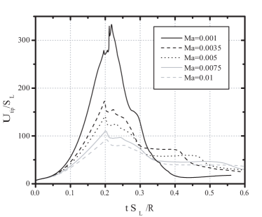
Figure 14: Scaled velocity of flame tip versus time for axisymmetric geometry, $\Theta=14$, and Mach numbers $Ma=0.001,\ 0.0035,\ 0.005,\ 0.0075,\ 0.01$.

An axisymmetric counterpart of Fig. 8 is shown in Fig. 9 with all parameters being the same except for the geometry. Isosurfaces are shown for $T=1400K$. The axisymmetic simulation also demonstrates the transition from a convex, “finger” flame front, to a concave “tulip” flame, accompanied by a significant reduction of the flame surface area and propagation velocity. Similar to Figs. 6 and 8, the flame tip curvature remains almost constant in a range of scaled times, $\tau_{sph}<\tau<\tau_{wall}$, corresponding to the later stage of finger flame acceleration.

In Figure 10 we present the scaled flame tip position versus time for the planar geometry with $\Theta=14$ and $Ma=0.001\sim 0.01$ in both linear and logarithmic scales. We see that the “exponential” nature of acceleration in the planar case is not very pronounced in the early stages, due to the relatively high value of $\tau_{sph}\approx 1/(\Theta-1)$ compared to its axisymmetric counterpart $\tau_{sph}\approx 1/(2\sqrt{\Theta(\Theta-1)})$ Bychkov.et.al-2007 ; the latter being approximately twice smaller for high values of $\Theta$ than in the planar case. Figure 11 shows the scaled velocity evolution for $\Theta=14$ and the planar geometry for a set of Mach numbers in the range $Ma=0.001\sim 0.01$. Here we see a significant dependence of the maximum flame tip velocity on the initial Mach number. At the same time, Fig. 11 shows that the scaled time of attaining the velocity maximum is almost independent of the Mach number, which can be demonstrated analytically, as follows. If we write the first-order correction to $\xi_{tip}$ in the form $\xi_{tip}=\xi_{tip,0}+Ma\xi_{tip,1}$, where $\xi_{tip,0}$ is given by Eq. (2.14), then Eq. (2.32) becomes

$$\vartheta = \Theta-Ma(\gamma-1)(\Theta-1)^{2}\left(\xi_{tip,0}+Ma\xi_{tip,1}+1\right)\approx$$

$$\approx \Theta-Ma(\gamma-1)(\Theta-1)\left[\Theta\exp{((\Theta-1)\tau)}-1\right].$$

Similarly, replacing $\tau$ in Eq. (4.2) by $\tau_{wall}$ in the form $\tau_{wall}=\tau_{wall,0}+Ma\tau_{wall,1}$, we find

$$\vartheta_{wall}\approx\Theta-Ma(\gamma-1)(\Theta-1)(\Theta^{2}-1).$$ (4.4)

Substituting Eq. (4.4) into Eq. (2.11), we obtain the estimation of $\tau_{wall}$ in the compressible case for the planar geometry:

$$\tau_{wall} = \frac{\ln\vartheta}{\vartheta-1}\approx$$

$$\approx \frac{\ln\Theta}{\Theta-1}\left[1+Ma(\gamma-1)(\Theta^{2}-1)\left(1-\frac{\Theta-1}{\Theta\ln\Theta}\right)\right].$$

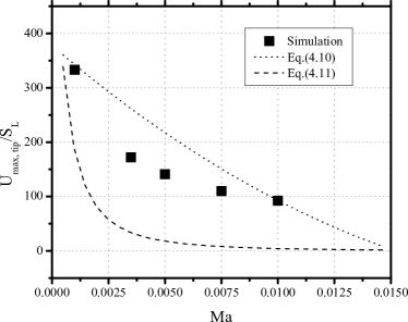
Figure 15: Scaled maximum flame tip velocity versus Mach number obtained in simulations for axisymmetric geometry, $\Theta=14$, compared to theoretical estrimates of Eqs. (4.2) and (4.11).

For typical $\Theta\approx 5\sim 10$ and $\gamma\approx 1.4$, the last term in Eq. (4.2) can be approximated as $\sim 0.2Ma\Theta^{2}$. Consequently, for small Mach numbers, $Ma\ll 5/\Theta^{2}\sim 0.1$, the quantity $\tau_{wall}=\ln\vartheta/(\vartheta-1)$ only slightly depends on $Ma$, which is substantiated by the simulation results of Fig. 11. The weak dependence of $\tau_{wall}$ on $Ma$ is convenient for evaluating the total time of the finger flame acceleration. We see from the simulation results of Figure 11 that the instant of the maximum flame tip velocity $\tau_{wall}$ only slightly increases with increasing $Ma$, remaining in the range $\tau_{wall}=2.2\sim 2.3$. Using the simplified analytical expression for $\tau_{wall}$ we can also estimate the maximum flame tip velocity from Eq. (2.41) and Eq. (2.44).

The peculiar feature of concurrent maximums of flame tip velocity for various initial Mach numbers can act as a useful criterion for the validity of $S_{L}$ and $Ma$ determined in the experiments. While in the numerical simulation we set $Ma$ as a parameter and obtain the concurrence of the maximum tip velocities mentioned above implicitly, analysis of the experimental data can encounter significant difficulties due to the uncertainty of $S_{L}$, as discussed in 4.1. Since $S_{L}$ is used in scaling time and velocity, even a small inaccuracy in its determination could lead to considerable shifting of the maximums of the tip velocity relative to each other. Thus, if the experimental conditions imply $R\approx R_{tip}\gg L_{f}$, i.e. pure curvature effect on flame tip velocity is insignificant at the later stages of the flame acceleration, the concurrence of the scaled flame tip velocity peaks could serve as an indication of correctly determined $S_{L}$ values for different $Ma$.

It is further noted that, similar to the experiments, in the present numerical simulations the initial flame velocity of a hemispherical flame front is considerably affected by the pure curvature effect, which can be seen from Fig. 11 for the flame tip velocity taken at $tS_{L}/R=0$. The initial flame radius in the numerical simulation is equal to $R_{init}=4.0L_{f}$; thus, similar to Eq. 4.2, we can estimate the correction to the initial flame velocity $S_{L,\,init}$ in the planar case, with the curvature term $\nabla\cdot\mathbf{n}=1/R_{init}$ in the form:

$$\frac{S_{L,\,init}}{S_{L}}=1-\frac{L_{f}}{R_{init}}=\frac{3}{4},$$ (4.6)

For $\Theta=14$, the initial tip velocity in the laboratory reference frame is $U_{tip}/S_{L}=\Theta S_{L,\,init}/S_{L}=0.75\Theta=10.5$, which is close to that observed in Fig. 11. However, the effect of pure curvature does not affect the present numerical simulations considerably, since we have taken relatively large channel widths, corresponding to $R=50\,L_{f}$ in the planar case, as specified in Sec. 3, which renders pure curvature effects to be negligible for all simulation runs.

Figure 12 shows the scaled maximum flame tip velocity versus the Mach number for the planar geometry and $\Theta=14$. Analytical estimates for the maximum flame tip velocity shown in Fig. 12 are calculated as follows. The first theoretical estimate for the maximum flame tip velocity accounts for all nonlinear terms of Eq. (2.41) and employs the exact solution, Eq. (2.46), as

$$\frac{U_{tip,\,max}}{S_{L}} = -Ma\gamma\left({\Theta-1}\right)^{2}\xi_{tip,\,wall}^{2}+$$ (4.7)

$$+ \sigma_{1,pl}\xi_{tip,\,wall}+\Theta_{1},$$

where $\xi_{tip,\,wall}$ is the flame tip position at time $\tau_{wall}$ calculated from Eq. (2.46), with $\tau=\tau_{wall}$. The second estimate is somewhat simplified accounting for the linear term only, derived from Eq. (2.44) as

$$\frac{U_{tip,\,max}}{S_{L}}=\sigma_{1,pl}\xi_{tip,\,wall}+\Theta_{1},$$ (4.8)

with $\xi_{tip,\,wall}=(\Theta_{1}/\sigma_{1,pl})\left[\exp{(\sigma_{1,pl}\tau_{wall})}-1\right]$. It is seen from Fig. 12 that predictions of the complete analytical solution, Eq. (4.7), and the solution accounting for the linear term only, Eq. (4.8), differ significantly, with the results of numerical simulation lying closer to the exact solution of Eq. (4.7). Most importantly, we see that both the simulation and theoretical results show significant reduction of the scaled maximum flame tip velocity with increasing initial Mach number, despite the fact that the non-scaled maximum tip velocity could be still increasing. Figure 12 shows that the influence of gas compressibility is noticeable for the estimation of the maximum flame velocity for finger-type flame acceleration, while previous theoretical studies Clanet.Searby-1996 ; Bychkov.et.al-2007 did not account for the significant reduction of the maximum scaled tip velocity for high initial Mach numbers. This is because they were conducted for slow methane-air flames, for which the effect of compressibility did not manifest itself.

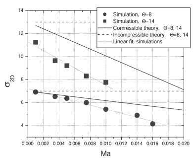
Figure 16: Scaled acceleration rate versus Mach number for planar geometry, $\Theta=8,\ 14$. Values of $\sigma_{1}$ obtained from numerical simulations are shown by circles for $\Theta=8$ and by squares for $\Theta=14$. Solid lines correspond to the theoretical dependencies give by Eq. (2.42), dashed line - to incompressible theory, see Eqs. (2.13)-(2.15), dotted lines - to linear fit of simulation data.

We next investigate acceleration of the finger-shaped flames at various values of the initial Mach number for the axisymmetric geometry. Figure 13 shows the scaled flame tip position versus time for the axisymmetric geometry for $\Theta=14$ and the Mach numbers $Ma=0.001\sim 0.01$, in both linear and logarithmic scales. It is seen that the stage of exponential flame acceleration is more distinctive in the axisymmetric geometry as compared to the planar case of Fig. 10. Figure 14 is the axisymmetric analogue of Fig. 11. Similar to the planar case, the maximum flame tip velocity strongly depends on the initial Mach number, but the time $\tau_{wall}$, when the maximum flame tip velocity is achieved, only depends on $Ma$ slightly. For $\Theta=14$ used in the simulation of Fig. 14, we have $\alpha\approx 13.5$, and Eq. (2.3) yields $\tau_{wall}\approx 0.15$. The numerical simulation of Fig. 14 shows somewhat delayed maximums of flame tip velocity with $\tau_{wall}\approx 0.2$, as compared to the theoretical prediction. This delay is attributed to the fact that for the axisymmetric case the effect of pure curvature is more pronounced in the initial stage of finger flame propagation, since the axisymmetric counterpart of Eq. (4.6) yields

$$\frac{S_{L,\,init}}{S_{L}}=1-\frac{2\,L_{f}}{R_{init}}=\frac{1}{2}.$$ (4.9)

However, in the axisymmetric case we have a wide domain with $R=75\,L_{f}$, see Sec. 3, which renders pure curvature effect at the later stage of finger flame acceleration negligible for all numerical runs in the axisymmetric case, resulting in concurrent peaks of the flame tip velocity in Fig. 14, similar to the planar case.

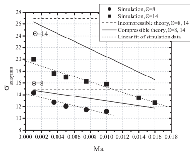
Figure 17: Scaled acceleration rate versus Mach number for axisymmetric geometry, $\Theta=8,\ 14$. Values of $\sigma_{1}$ obtained from numerical simulations are shown by circles for $\Theta=8$ and by squares for $\Theta=14$. Solid lines correspond to the theoretical dependencies given by Eq. (2.72), dashed line - to incompressible theory (see Eq. (2.56)), dotted lines - to linear fit of simulation data.

An axisymmetric counterpart of Fig. 12 is presented in Fig. 15. Contrary to the planar case, the theoretical estimate of the maximum tip velocity shown in Fig. 15 is related to two opposite limiting cases descrbed in Sec. 2.3. The first estimate is obtained from Eq. (2.68) as

$$\frac{U_{tip,\,max}}{S_{L}}=\{2\alpha_{1}\tanh\left(\alpha_{1}\tau_{wall}\right)-$$

$$-2Ma\,\alpha\left[1+\gamma\left(\Theta-1\right)\right]\}\xi_{tip,\,wall}+\Theta_{1},$$ (4.10)

where the flame tip position $\xi_{tip,\,wall}$ at $\tau=\tau_{wall}$ is calculated from Eq. (2.3) while $\sigma_{1,axi}$ and $\Theta_{1}$ are given by Eqs. (2.72) and (2.43), respectively. For the second limiting case of late stage acceleration, the flame tip velocity estimate is given by Eq. (2.70) as

$$\frac{U_{tip,\,max}}{S_{L}}=-2Ma(\Theta - 1)(2\Theta\gamma-\gamma+1)\xi_{tip,\,wall}^{2}+$$ (4.11)

$$+ \sigma_{1,axi}\xi_{tip,\,wall}+\Theta_{1},$$

where the flame tip position $\xi_{tip,\,wall}$ at $\tau=\tau_{wall}$ is calculated from Eq. (2.73). We see that results of the numerical simulation in most cases are located in between the values given by Eqs. (4.2) and (4.11), as suggested in Sec. 2.3, although, this tendency appears to change for higher values of $Ma$.

Figure 16 shows the scaled acceleration rate versus Mach number for the planar geometry, with $\Theta=8,\ 14$. It is seen that the agreement between theory and simulations is significantly better for $\Theta=8$, indicating that the role of gas compressibility increases both with $Ma$ and $\Theta$. Furthermore, Fig. 16 shows that the growth rate $\sigma$ significantly decreases with increasing $Ma$, and the isobaric theoretical model of the finger-flame acceleration, Refs. Clanet.Searby-1996 ; Bychkov.et.al-2007 , noticeably overestimates the acceleration rate $\sigma$ for high-$Ma$ flames. We next note that an accurate estimate of the acceleration rate is of crucial importance, e.g., for the analysis of flame-generated shocks, preheating of the fuel mixture, pre-detonation run-up distance and the DDT onset Bychkov-Akkerman-2006 ; Valiev.et.al-2008 . Figure 17 shows the scaled acceleration rate versus the Mach number for the axisymmetric geometry, with $\Theta=8$ and 14. Similar to the planar case of Fig. 16, the agreement of theory and simulations is better for $\Theta=8$ than for $\Theta=14$, which indicates a more important role of the compressibility effects for larger $\Theta$. For $\Theta=14$ we have even more significant deviation of the numerical data from the theoretical predictions as compared to the planar case. Still, the trend remains the same: $\sigma$ decreases quite rapidly with increasing $Ma$.

$\phi$	$\Theta$	$S_{L}$, cm/s	$c_{s}$ m/s	$Ma$	$1/t$, $\rm{s}^{-1}$	$\sigma_{1}$
1.0	8.02	41.8	340	0.00123	132.6	15.8
					129.7	15.5

Table 2: Experimental values of $\sigma_{1}$ obtained from Ref. Clanet.Searby-1996 , for $\Theta\approx 8$, low-Mach propane-air mixture and axisymmetric geometry. $\phi$ is mixture equivalence ratio, $c_{s}$ is sound speed in unburnt gas mixture, $1/t$ is experimentally measured tulip flame growth rate (for two experimental runs).

Figure 18 shows the comparison of the scaled acceleration rates obtained in simulations for the planar and axisymmetric geometries, for $\Theta=8$ in both cases; the experimental results for $\sigma_{1}$ obtained in the present work and those of Ref. Clanet.Searby-1996 are also shown. The latter experimental data is summarized in Table 2 for two experimental runs for neutrally stable ($\phi=1.0$) low-$Ma$, propane-air mixture with $\Theta=8.02$, and axisymmetric geometry of the tube. We see from Fig. 18 that the scaled acceleration rate $\sigma_{1}$ obtained in the present experiments for the high-$Ma$ $H_{2}/O_{2}$ stoichiometric mixture in a channel with a quadratic cross-section are considerably closer to the planar case than the axisymmetric one. Thus, although the flame tip has the hemispherical shape, the global flame front acceleration is governed by the quadratic cross section of the channel and can be described by the theory of Section 2.1. At the same time, values of $\sigma_{1}$ of Table 2 Clanet.Searby-1996 for low-$Ma$, propane-air mixtures are close to the incompressible value $\sigma_{0}$ for the axisymmetric case, in agreement with the present theory. It is known that flame acceleration in DDT sensitively depends on flame confinement and the channel geometry Wu-2012 . The present numerical simulation and experimental results indicate that the geometry of the tube affects the growth rate of finger flame acceleration significantly, with the axisymmetric tube being favorable for faster flame acceleration due to the finger flame mechanism.

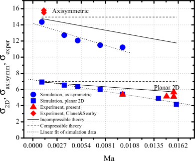
Figure 18: Comparison of scaled acceleration rates versus Mach number for experiments and simulations for planar and axisymmetric geometries, $\Theta=8$. Values of $\sigma_{1}$ obtained from numerical simulations are shown by circles for axisymmetric geometry and by squares for planar geometry. Triangles show experimental results of Table 1, diamonds - of Ref. Clanet.Searby-1996 , see Table 2. Solid lines correspond to the theoretical dependencies given by Eq. (2.42) (planar) and Eq. (2.72) (axisymmetric), dashed line - to incompressible theory, see Eq. (2.15) (planar) and Eq. (2.56) (axisymmetric), dotted lines - to linear fit of simulation data.

We conclude the present extensive investigation by noting that pressure jump at the flame front could potentially induce a gas velocity of $O(S_{L})$, and as such the pressure field could play an essential role in the present phenomena of interest Law-2006 ; Higuera-2009 . Here we recognize that the present theoretical results are obtained by considering only two (quasi-planar) parts of the flame: 1) flame skirt near the closed tube end, and 2) flame tip in the vicinity of channel axis. Due to the exponential acceleration of the flame tip, the entire process of finger flame propagation occurs rapidly. For example, for $\Theta=8$ the characteristic non-dimensional time of reaching the maximum flame tip velocity in planar geometry is $\tau_{wall}\sim 0.25$. By that instant the flame tip has shifted to the non-dimensional position $\xi_{tip}=\Theta$. If we assume that the pressure field induces flame velocity of the order of $S_{L}$ at the curved parts of the flame (i.e. not at the skirt and the flame tip), then at the end of the finger flame evolution the additional displacement of the curved elements of the flame would be of the order of $S_{L}t_{wall}=S_{L}\tau_{wall}R/S_{L}\sim 0.25$ (in nondimensional units), i.e. considerably smaller than the flame tip displacement $\xi_{tip}=\Theta$. Due to the elongated flame shape resulting from the exponential flame tip acceleration, the motion of the curved parts of the flame front does not considerably influence the flame acceleration. Consequently, pressure field variation has only minimal influence on the present theory. It is also noted that since our problem is evolutionary (non-steady), the maximum flame tip velocity could be more than two orders of magnitude higher than $S_{L}$, hence implying that the low-Mach limit is not applicable, and the pressure field cannot be considered steady as, for example, in Bunsen flame problem Higuera-2009 . This is beyond the scope of the present investigation.

$\Delta z_{f}/L_{f}$	$U_{max}/S_{L}$	$\Delta U_{max}/S_{L}$	$t_{max}S_{L}/R$	$\Delta t_{max}S_{L}/R$	$Z_{tip,*}/R$	$\Delta Z_{tip,*}/R$
1.0	31.14		0.3265		4.5095
0.5	34.68	3.54	0.3032	0.2706	5.282	0.7725
0.25	36.171	1.43	0.2973	0.0059	5.441	0.159
0.125	36.85	0.679	0.2965	0.0008	5.474	0.033

Table 3: Resolution tests for planar geometry, $Ma=0.005$, $\Theta=8$.

Finally, it is also noted that the influence of gas compressibility on the flame acceleration obtained in the present paper is qualitatively different from that of the DL instability in compressible gases and plasmas Travnikov-1997 ; Travnikov-1999 ; Modestov-2009 . The compressibility effect renders the DL instability much stronger in both linear and nonlinear stages, while in the case of finger flame acceleration compressibility moderates flame acceleration in tubes considerably.

5 Conclusions

The theory, experiments and numerical simulations of the present work show that the growth rate $\sigma$ of the finger-flame acceleration from the closed end of a channel/tube decreases significantly with increasing initial Mach number, $Ma$. Hence, previous theoretical estimates of Clanet.Searby-1996 ; Bychkov.et.al-2007 , derived with the incompressible approximation, overestimate $\sigma$ for flames with high laminar burning velocities, such as the $H_{2}/O_{2}$ or acetylene/air flames. In the present study, we account for gas compression through expansion for small Mach number up to first-order terms, and validate the theoretical analysis by numerical simulations and experiment. The present numerical simulation and theory show that the maximum flame tip velocity significantly depends on $Ma$, with the scaled time of the maximum flame tip velocity being almost independent of it. The present results collectively demonstrate that the geometry of the channel affects the growth rate of the finger flame significantly, with the axisymmetric channel being more conducive for fast initial flame acceleration from the closed end in channels with smooth walls. It is emphasized that compressibility effects should be taken into account when estimating the strength of shock waves generated by the initial finger-type flame acceleration, pre-heating of the unburnt fuel mixture ahead of the flame, the DDT onset time and position.

6 Acknowledgements

The authors are grateful to Fujia Wu and Hemanth Kolla for useful discussions. This work was supported by the Swedish Research Council (VR) and Stiftelsen Lars Hiertas Minne grant FO2010-1015. Numerical simulations were performed at the High Performance Computer Center North (HPC2N), Umeå, Sweden, through the SNAC project 001-10-159. Participation of Princeton University was supported by the US Air Force Office of Scientific Research.

7 Appendix: Resolution and laminar velocity tests

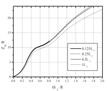
Figure 19: Flame tip position versus time for different values of the mesh size. Thick solid line correspond to $\Delta z_{f}/L_{f}=0.125$, dashed line - to $\Delta z_{f}/L_{f}=0.25$, thin solid line - to $\Delta z_{f}/L_{f}=0.5$, dotted line - to $\Delta z_{f}/L_{f}=1.0$

In order to check if the adopted resolution is sufficient to study the flame acceleration process, we performed the resolution tests for the primary results for $Ma=0.005$. The grid size in the flame domain varied between $0.125L_{f}$, $0.25L_{f}$, $0.5L_{f}$ and $1L_{f}$. We checked the velocity of the flame tip at the instants corresponding to the state of the maximum flame tip velocity, as well as the flame tip position at the time instant $tS_{L}/R=0.303$. The resolution test results are presented in Table 3 and in Figs. 19 and 20.

Notation: $\Delta z_{f}/L_{f}$ is the spatial step in the flame grid domain; $U_{max}/S_{L}$ maximum flame tip velocity (see Fig. (20)); $t_{max}S_{L}/R$ scaled time moment corresponding to the maximum of flame tip velocity; $Z_{tip,*}/R$ flame tip position at time $t_{*}S_{L}/R=0.303$ (see Fig. (20)). $\Delta U_{max}/S_{L}$ increment of $U_{max}/S_{L}$ calculated in the table row $i$ as $\Delta U_{max}(i)=U_{max}(i)-U_{max}(i-1)$. Increments for $t_{max}S_{L}/R$ and $Z_{tip,*}/R$ are calculated in a similar manner. Resolution in the wave grid domain is equal to $\Delta z_{w}=2\times\Delta z_{f}$ for each run.

Table 3 and Figs. 19 and 20 show good convergence of the numerical solution with the increase of mesh resolution. Resolution tests also showed convergence of time corresponding to the maximum flame tip velocity with increasing resolution.

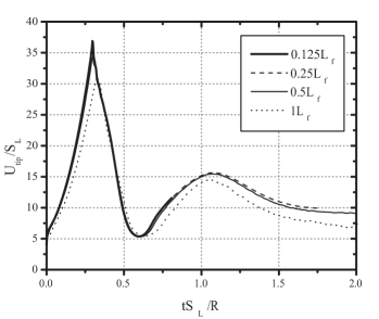
Figure 20: Velocities of the flame tip versus time for different values of the mesh size. Thick solid line correspond to $\Delta z_{f}/L_{f}=0.125$, dashed line - to $\Delta z_{f}/L_{f}=0.25$, thin solid line - to $\Delta z_{f}/L_{f}=0.5$, dotted line - to $\Delta z_{f}/L_{f}=1.0$

In addition to the resolution tests, laminar flame velocity tests were performed for $Ma=0.001,\ \Theta=8,\ 14$. The numerical setup was similar to the main numerical experiments, except for planar initial flame front and tube width $2R=4L_{f}$. That value was chosen to be below the critical diameter needed for the growth of the hydrodynamic instability Liberman.et.al-2003 , so that the flame front remains planar during the test simulation. For $\Theta=14$, the measured laminar planar flame velocity in laboratory frame was $U_{f,\ lab}/S_{L}=13.97\pm 0.03$; for $\Theta=8$ $U_{f,\ lab}/S_{L}=7.97\pm 0.05$.

References

- (1) Zeldovich Ya. B., Barenblatt G. I. , Librovich V. B., Makhviladze G. M. (1985) The Mathematical Theory of Combustion and Explosions. New York: Consultants Bureau.
- (2) Law C. K. (2006) Combustion Physics. New York: Cambridge University Press.
- (3) Roy G.D. , Frolov S.M. , Borisov A.A., Netzer D.W., (2004) Prog. Energy Combust. Sci. 30, 545
- (4) Ciccarelli, G., Dorofeev, S. (2008) Prog. Energy Combust. Sci., 34(4), 499-550
- (5) Dorofeev S.B. (2011) Proc. Comb. Inst., 33, 2161-2175
- (6) Shelkin K., (1940) J. Exp. Theor. Phys., 10, 823.
- (7) Bychkov V., Valiev. D., Eriksson L.-E., (2008) Phys. Rev. Lett., 101, 164501.
- (8) Bychkov V., Petchenko A., Akkerman V., Eriksson L.-E., (2005) Phys. Rev. E, 72, 046307.
- (9) Akkerman V., Bychkov V., Petchenko A., Eriksson L.-E., (2006) Combust. Flame, 145, 206.
- (10) Valiev D., Bychkov V. , Akkerman V. , Law C. K., Eriksson L.-E. (2010) Combust. Flame, 157, 1012-1021
- (11) Clanet C. , Searby G. (1996) Combust. Flame, 105, 225-238.
- (12) Bychkov V., Akkerman V. , Fru G., Petchenko A. , Eriksson L.-E. (2007) Combust. Flame, 150, 263-276.
- (13) Xiao H., Makarov D., Sun J., Molkov V. (2012) Combust. Flame, 159, Issue 4, 1523–1538
- (14) Xiao H., Wang Q., He X., Sun J., Shen X. (2011) Int. J. Hydrogen Energy, 36, Issue 10, 6325–6336
- (15) Nkonga B., Fernandez G. , Guillard H. , Larrouturou B. (1993) Comb. Sci. Tech. 87, 69-89.
- (16) Oppenheim A. K. , Ghoniem A. F. (1983) In 21st Aerospace Sciences Meeting AIAA-83-0470. Reno, Nevada.
- (17) Pizza, G., Frouzakis C. E., Mantzaras J., Tomboulides A. G., Boulouchos K. (2010) Journal of Fluid Mechanics, 658, 463
- (18) Gonzalez M., Borghi R., Saouab A. (1992) Combust. Flame, 88, 201.
- (19) Gonzalez M. (1996) Combust. Flame, 107, 245.
- (20) Petchenko A., Bychkov V., Akkerman V., Eriksson L.-E. (2006) Phys. Rev. Lett. 97, 164501.
- (21) Petchenko A. , Bychkov V., Akkerman V., Eriksson L.-E. (2007) Combust. Flame 149, 418-434.
- (22) Akkerman V., Bychkov V., Petchenko A., Eriksson L.-E. (2006) Combust. Flame 145, 675-687.
- (23) Akkerman V., Law C.K., Bychkov V., Eriksson L.-E.(2010) Phys. Fluids 22 (5), 053606.
- (24) Kuznetsov M., Liberman M., Matsukov I. (2010) Comb. Sci. Tech. 182, 1628 - 1644.
- (25) Wu M. , Burke M., Son S., Yetter R. (2007) Proc. Combust. Inst. 31, 2429.
- (26) Cicarelli G. , Johansen C., Parravani M. (2010) Combust. Flame 157, 2125.
- (27) Kuznetsov M., Alekseev V. , Matsukov I., Dorofeev S. (2005) Shock Waves 14, 205-215.
- (28) Landau L. D. , Lifshitz. E. M. (1993) Fluid mechanics. Oxford ; New York: Pergamon Press.
- (29) Chue R., Clarke J., Lee J.H. (1993) Proc. R. Soc. Lond. A 441 607 .
- (30) Bychkov V. and Akkerman V., (2006) Phys. Rev. E. 73, 066305.
- (31) Valiev D. M., Bychkov V. , Akkerman V., Eriksson L.-E. (2009) Phys. Rev. E, 80(3), 036317.
- (32) Bychkov V., Akkerman V. , Valiev D., Law C. K. (2010) Combust. Flame, 157, 2008-2011.
- (33) Bychkov V., Akkerman V. Valiev D. , Law C. K. (2010) Phys. Rev. E, 81, 026309.
- (34) Liberman, M.A., Ivanov M.F., Peil O.E., Valiev D.M., Eriksson L.-E. (2003) Combustion Theory And Modelling, 7, Issue 4, 653-676.
- (35) Poinsot T., Veynante D., 2001. Theoretical and Numerical Combustion, R.T. Edwards.
- (36) Valiev D., Bychkov V. , Akkerman V., Eriksson L.-E., Marklund M. (2008) Phys. Lett. A 372, Issues 27-28, 4850-4857
- (37) Wollblad C., Davidson L. , L.-E. Eriksson (2006) AIAA Journal, 44, 2340-2353.
- (38) Kee R.J., Rupley F.M., Miller J.A. (1991) CHEMKIN-II: A FORTRAN Chemical Kinetics Package for the Analysis of Gas-Phase Chemical Kinetics, Technical Report SAND89-8009B, UC-706, Sandia National Laboratories, Albuquerque, New Mexico
- (39) Burke M.P., Chaos M., Ju Y., Dryer F.L., and Klippenstein S.J. (2012) ”Comprehensive H2/O2 Kinetic Model for High-Pressure Combustion”, International Journal of Chemical Kinetics 44, Issue 7, 444-474.
- (40) Kagan L., Sivashinsky G. (2003) Combust. Flame 134 389 .
- (41) Bychkov V., Matyba P., Akkerman V., Modestov M., Valiev D., Brodin G., Law C.K., Marklund M., Edman L. (2011) Phys. Rev. Lett. 107, 016103.
- (42) Bychkov V., Jukimenko O., Modestov M., Marklund M., (2012) Phys. Rev. B 85, 245212.
- (43) Decelle W., Vanacken J., Mochalkov V., Tejada J., Hernandez J., Macia F. (2009) Phys. Rev. Lett. 102, 027203.
- (44) Modestov M., Bychkov V., Marklund M. (2011) Phys. Rev. Lett. 107, 207208.
- (45) Wu M.-H., Kuo W.-C. (2012) Combust. Flame 159, Issue 3, 1366-1368.
- (46) Higuera F.J. (2009) Combustion and Flame, 156, pp 1063 - 1067
- (47) Travnikov O.Yu., Liberman M.A., Bychkov V.V. (1997) Phys. Fluids, 9, 3935
- (48) Travnikov O.Yu., Bychkov V.V., Liberman M.A. (1999) Phys. Fluids, 11, 2657
- (49) Modestov M., Bychkov V., Valiev D., Marklund M. (2009) Phys. Rev. E, 80, 046403