Universal anomalous diffusion of weakly damped particles

Abstract

We show that anomalous diffusion arises in two different models for the motion of randomly forced and weakly damped particles: one is a generalisation of the Ornstein-Uhlenbeck process with a random force which depends on position as well as time, the other is a generalisation of the Chandrasekhar-Rosenbluth model of stellar dynamics, encompassing non-Coulombic potentials. We show that both models exhibit anomalous diffusion of position $x$ and momentum $p$ with the same exponents: $\langle x^{2}\rangle\sim C_{x}t^{2}$ and $\langle p^{2}\rangle\sim C_{p}t^{2/5}$. We are able to determine the prefactors $C_{x}$, $C_{p}$ analytically.

I Introduction

In many systems the growth of a dynamical variable $X$ with time $t$ satisfies $\langle X^{2}\rangle\sim Ct^{\alpha}$ where the angular brackets denote averaging. The process is said to be anomalous diffusion if $\alpha\neq 1$. Anomalous diffusion may be a consequence of a power-law built into the dynamical process, such as in Lévy flight models Met+00 , or it may be an ‘emergent’ property, where the anomalous exponent $\alpha$ is not a direct consequence of power laws which are built into the model. The latter case is more interesting, because non-integer exponents do not feature in the fundamental laws of physics, but there are relatively few models where ‘emergent’ anomalous diffusion can be analysed exactly. In this paper we describe two physically natural models for the diffusion of a particle which is accelerated by random forces. If the damping is sufficiently weak the particle can exhibit anomalous diffusion, having universal exponents, the same for each model.

Our two models are generalisations of two classic models for diffusion processes. The first is an extension of the Ornstein-Uhlenbeck process Uhl+30 , in which a particle is subjected to a rapidly fluctuating random force, and is damped by viscous drag. In the generalised Ornstein-Uhlenbeck process the random force depends upon the position of the particle and time and is derived from a potential $\Phi(\mbox{\boldmath$x$},t)$. Earlier works analysed this model in detail for one spatial dimension Arv+05 ; Bez+06 . This model exhibits anomalous diffusion in one dimension. Here we discuss higher spatial dimensions, where the mechanism for anomalous diffusion is significantly different, as was suggested (for a closely related model) in Gol+91 ; Ros92 . Here we obtain exact formulae for the momentum distribution of the generalised Ornstein-Uhlenbeck process in two and three dimensions (for a particle which is initially at rest). We use these to obtain precise asymptotic formulae for the growth of the second moment of the coordinate: the second moments scale as $\langle p^{2}\rangle\sim t^{2/5}$ and $\langle x^{2}\rangle\sim t^{2}$ in the anomalous diffusion regime (the exponents are the same as those obtained in Ros92 ; we obtain the prefactor exactly).

We also discuss an extension of the Chandrasekhar-Rosenbluth model for diffusion Cha43 ; Ros+57 , in which a test particle interacts with a gas of point masses via a pair potential. The interaction should cause small changes of momentum, which can be modelled as a diffusion process. Usually the interaction is gravitational, and the application is to the motion of stars in galaxies, but here we simplify the problem by considering a non-singular weak interaction potential. We show that, surprisingly, the diffusion tensor has the same form as for the generalised Ornstein-Uhlenbeck process, and that consequently there is anomalous diffusion with the same universal exponents. For this model too, we derive diffusion coefficients for this model precisely in terms of the microscopic parameters.

The anomalous diffusion effect which we describe is analysed by introducing a diffusion process describing the fluctuations of the momentum $p$ of a particle in response to a spatially and temporally fluctuating random potential. The diffusion coefficient of this process, $D(p)$, is a function of the momentum of the particle. We remark that this approach to formulating the equation of motion was first introduced by Sturrock Stu66 , and that similar developments appeared later in the mathematical literature (see Agu+09 and references cited therein). Our paper is the first work to give a solution to the generalised Ornstein-Uhlenbeck process in two or three dimensions.

II Generalised Ornstein-Uhlenbeck model

We consider a particle of mass $m$ with momentum $p$ subjected to the generalised Ornstein-Uhlenbeck process Bez+06 . This is described by equations of motion

$$\dot{\mbox{\boldmath$x$}}=\frac{\mbox{\boldmath$p$}}{m}\ ,\ \ \ \dot{\mbox{\boldmath$p$}}=-\gamma\mbox{\boldmath$p$}+\mbox{\boldmath$f$}(\mbox{\boldmath$x$},t)$$ (1)

where $x$ is the particle’s position. The particle experiences two types of forces: a drag force $-\gamma\mbox{\boldmath$p$}$ with $\gamma$ being a damping rate and a random force $\mbox{\boldmath$f$}(\mbox{\boldmath$x$},t)$. Unlike the classic Ornstein-Uhlenbeck process, where the force depends only upon time, in our generalised model the random force depends upon the position as well. We assume that $\mbox{\boldmath$f$}(\mbox{\boldmath$x$},t)$ is a force derived from a random potential varying in time and space, i.e. $\mbox{\boldmath$f$}(\mbox{\boldmath$x$},t)=-\nabla\Phi(\mbox{\boldmath$x$},t)$, where $\Phi(\mbox{\boldmath$x$},t)$ has statistics

$$\langle\Phi(\mbox{\boldmath$x$},t)\rangle=0\ ,\ \langle\Phi(\mbox{\boldmath$x$},t)\Phi(\mbox{\boldmath$x$}^{\prime},t^{\prime})\rangle=C(|\mbox{\boldmath$x$}-\mbox{\boldmath$x$}^{\prime}|,|t-t^{\prime}|)\ .$$ (2)

The correlation function $C(x,t)$ has temporal and spatial scales, $\tau$ and $\xi$, respectively. We consider the case where $\gamma\tau\ll 1$, implying that the momentum satisfies a diffusion equation. We define a momentum scale $p_{0}=m\xi/\tau$, such that if $|\mbox{\boldmath$p$}|\gg p_{0}$ the force experienced by the particle decorrelates much more rapidly than the force experienced by a stationary particle. We consider the limit where $|\mbox{\boldmath$p$}|\gg p_{0}$, which is realised for weak damping. The dynamics of (1) can be described by a diffusion equation for the probability density of the momentum, $P(\mbox{\boldmath$p$},t)$: we now consider how to derive this diffusion equation.

The dynamics of the momentum can be approximated by a Langevin process. Small increments of components $p_{i}$ of the momentum vector $p$ may be written as

$$\delta p_{i}=-\gamma p_{i}\delta t+\delta w_{i}$$ (3)

where $\delta w_{i}$ is the impulse exerted by the $i$-th component of the force $f$ on the particle in time $\delta t$,

$$\delta w_{i}(t_{0}) = \int_{t_{0}}^{t_{0}+\delta t}{\rm d}t_{1}\ f_{i}(\mbox{\boldmath$x$}(t_{1}),t_{1})$$ (4)

$$= \int_{t_{0}}^{t_{0}+\delta t}{\rm d}t_{1}\ f_{i}(\mbox{\boldmath$p$}t_{1}/m,t_{1})+O(\delta t^{2})\ .$$

The Langevin process (3) is equivalent to the Fokker-Planck equation describing time evolution of the probability density of momentum $P(\mbox{\boldmath$p$},t)$. In order to construct the equation we need to know drift and diffusion coefficients, $v_{i}=\langle\delta p_{i}\rangle/\delta t$ and $D_{ij}=\langle\delta p_{i}\delta p_{j}\rangle/2\delta t$ respectively. Using the definition of the increment $\delta w_{i}$ we find

$$\langle\delta w_{i}\delta w_{j}\rangle \sim \int_{0}^{\delta t}{\rm d}t_{1}\int_{0}^{\delta t}{\rm d}t_{2}\langle f_{i}(\mbox{\boldmath$p$}t_{1}/m,t)f_{j}(\mbox{\boldmath$p$}t_{2}/m,t_{2})\rangle$$ (5)

$$\sim \delta t\int_{-\infty}^{\infty}{\rm d}t_{1}\ \langle f_{i}(\mbox{\boldmath$0$},0)f_{j}(\mbox{\boldmath$p$}t_{1}/m,t_{1})\rangle$$

$$= 2D_{ij}\delta t$$

(the second step is justified when $\delta t$ is large compared to $\tau$ but small compared to $\gamma^{-1}$).

The components $D_{ij}$ of the momentum diffusion tensor ${\bf D}$ depend upon the direction of the momentum. For the case where the momentum is aligned with the $x$-axis (that is, where $\mbox{\boldmath$p$}=p{\bf e}_{1}$, the coefficients of the diffusion matrix are expressed in terms of the correlation function of the potential as follows:

$$D_{xx} = -\frac{m}{2p}\int_{-\infty}^{\infty}{\rm d}R\ \frac{\partial^{2}C}{\partial R^{2}}(R,mR/p)$$

$$D_{yy} = -\frac{m}{2p}\int_{-\infty}^{\infty}{\rm d}R\ \frac{1}{|R|}\frac{\partial C}{\partial R}(R,mR/p)$$

$$D_{xy} = 0\ .$$ (6)

(In three dimensions $D_{zz}=D_{yy}$ and $D_{xz}=D_{yz}=0$.) For other directions of the momentum, the elements of the momentum diffusion tensor can be obtained by applying a rotation matrix. If ${\bf O}$ is a rotation matrix which rotates the momentum vector $p$ into $\mbox{\boldmath$p$}^{\prime}={\bf O}\mbox{\boldmath$p$}=p{\bf e}_{1}$ which is aligned with the $x$-axis, then the elements $D^{\prime}_{ij}$ of the diffusion matrix in the transformed coordinate system are given by (II). The diffusion matrix in the original coordinate system is ${\bf D}={\bf O}\,{\bf D}^{\prime}\,{\bf O}^{\rm T}$.

Having considered the diffusive fluctuations of the momentum, we now consider its drift, $\langle\delta p_{i}\rangle=-\gamma p_{i}\delta t+\langle\delta w_{i}\rangle$. Expanding $f_{i}(\mbox{\boldmath$x$},t)$ we obtain (in $d$ dimensions)

$$f_{i}(\mbox{\boldmath$x$},t)=f_{i}(\mbox{\boldmath$0$},t)+\sum_{j=1}^{d}\frac{\partial f_{i}(\mbox{\boldmath$0$},t)}{\partial x_{j}}x_{j}(t)$$ (7)

where $x_{j}(t)$ can be written as a solution of (1),

$$x_{j}(t) = \frac{1}{m}\int_{0}^{t}{\rm d}t_{1}\int_{0}^{t_{1}}{\rm d}t_{2}\ {\rm exp}[-\gamma(t_{1}-t_{2})]$$ (8)

$$\times f_{j}(\mbox{\boldmath$p$}t_{2}/m,t_{2})\ .$$

Combining together (4), (7) and (8) we obtain

$$\langle\delta w_{i}\rangle \sim \frac{1}{m}\sum_{j=1}^{d}\int_{0}^{\delta t}{\rm d}t_{1}\int_{0}^{t_{1}}{\rm d}t_{2}\int_{0}^{t_{2}}{\rm d}t_{3}\ \exp[-\gamma(t_{2}-t_{3})]$$ (9)

$$\times\bigg{\langle}\frac{\partial f_{i}(\mbox{\boldmath$0$},t_{1})}{\partial x_{j}}f_{j}(\mbox{\boldmath$p$}t_{3}/m,t_{3})\bigg{\rangle}\ .$$

We approximate ${\rm exp}[-\gamma(t_{2}-t_{3})]$ by unity for $\gamma\tau\ll 1$, and use the assumption that $\delta t\gg\tau$ to obtain

$$\langle\delta w_{i}\rangle \sim \frac{\delta t}{2m}\sum_{j=1}^{d}\int_{-\infty}^{\infty}{\rm d}t\ t\bigg{\langle}\frac{\partial f_{i}(\mbox{\boldmath$0$},0)}{\partial x_{j}}f_{j}(\mbox{\boldmath$p$}t/m,t)\bigg{\rangle}$$ (10)

$$= \delta t\sum_{j=1}^{d}\frac{\partial}{\partial p_{j}}D_{ij}(\mbox{\boldmath$p$})\ .$$

Taking account of the fact that the drift coefficients contain derivatives of the diffusion coefficients, we obtain the Fokker-Planck equation,

$$\frac{\partial P}{\partial t}=\frac{\partial}{\partial\mbox{\boldmath$p$}}\cdot\left(\gamma\mbox{\boldmath$p$}+{\bf D}(\mbox{\boldmath$p$})\frac{\partial}{\partial\mbox{\boldmath$p$}}\right)P\ .$$ (11)

We are primarily interested in the case of weak damping, where the typical momentum satisfies $|\mbox{\boldmath$p$}|\gg p_{0}$. In this limit, the diffusion coefficients have an algebraic dependence upon $p=|\mbox{\boldmath$p$}|$. For diffusion of the momentum vector parallel to its direction, when $p\gg p_{0}$ the leading term is of order $p^{-3}$ and the result is given by

$$D_{xx}\sim\frac{D_{3}p_{0}^{3}}{p^{3}},\;\;\;D_{3}=-\frac{m^{3}}{4p_{0}^{3}}\int_{-\infty}^{\infty}{\rm d}RR^{2}\frac{\partial^{4}C}{\partial R^{2}\partial t^{2}}(R,0)\ .$$ (12)

For diffusion of $p$ in a direction perpendicular to its direction, we have

$$D_{yy}\sim\frac{D_{1}p_{0}}{p},\;\;\;D_{1}=-\frac{m}{2p_{0}}\int_{-\infty}^{\infty}{\rm d}R\ \frac{1}{|R|}\frac{\partial C}{\partial R}(R,0)\ .$$ (13)

Note that when $p\gg p_{0}$, the diffusion of the direction of the momentum vector is much more rapid than diffusion of its magnitude. This makes the behaviour of the generalised Ornstein-Uhlenbeck process in two or more dimensions very different from its behaviour in one dimension.

Results equivalent to (12) and (13) were obtained in Gol+91 ; Ros92 in an analysis of a closely related model.

III Generalised Chandrasekhar-Rosenbluth model

In this section we consider motion of a particle travelling through an infinite homogeneous population of background particles. We assume that the test particle interacts with the background particles, and the background particles do not interact with each other. As the test particle moves, its interaction with each of the background particles causes small changes of its velocity. When the number of the background particles is very large, the velocity of the test particle changes rapidly and in an unpredictable way, so that its motion can be described by a diffusion process. The test particle could be a star moving in a galaxy interacting with the background stars (the interaction between the background stars is not considered), so that the force of interaction is gravitational and thus proportional to the inverse square of the distance $r$ between stars. This problem was originally studied by Chandrasekhar Cha43 , who found that the test particle experiences a gradual decrease of the velocity in the direction of motion. This phenomenon is called ‘dynamical friction’. For ‘slow’ particles (with velocities much smaller than some representative velocity scale) this deceleration is proportional to the velocity of the particle $v$ (analogous to the Stokes’s law for a drag force for a particle is a viscous medium). For sufficiently ‘fast’ particles the deceleration is proportional to $v^{-2}$.

Subsequently, Rosenbluth et al. Ros+57 studied the diffusion of momentum of the test particle in this model in greater depth. They found that in the ‘fast’ regime the diffusion coefficient of the momentum in the direction parallel to the direction of motion is proportional to $v^{-3}$, while the diffusion coefficients in the plane perpendicular to the direction of motion is proportional to $v^{-1}$. These dependences are equivalent to the momentum dependences of the radial and transverse fluctuations of the momentum in the generalised Ornstein-Uhlenbeck model, obtained in equations (12) and (13). The expressions for these diffusion coefficients obtained in Ros+57 contain logarithmic terms due to the long-ranged nature of the Coulombic potential, which makes it difficult to write down precise formulae. In order to illuminate the relation between the generalised Ornstein-Uhlenbeck model and the Chandrasekhar-Rosenbluth model in the simplest context, in this section we consider the latter model for the case when the interaction is described by a short-range potential $U(r)$ of some rather general radially symmetric form. We obtain precise expressions for these diffusion coefficients and show that the results for the scaling of the diffusion coefficients are the same as in the generalised Ornstein-Uhlenbeck process. This leads to the same anomalous diffusion behaviour in both models.

We shall only discuss the two-dimensional case for simplicity and proceed as follows (some of the presentation adapts the discussion of the Chandrasekhar model in Bin+94 ). We first calculate the change of the velocity of a test particle due to the encounter with a stationary background particle. We denote components of this change by $\Delta v^{\prime}_{\parallel}$ and $\Delta v^{\prime}_{\perp}$, in the directions parallel and perpendicular to the initial velocity of the test particle. Next, we consider the change of the velocity of the test particle for the case when the background particle propagates with velocity $\mbox{\boldmath$v$}_{b}$. We denote components of this change by $\Delta v_{\parallel}$ and $\Delta v_{\perp}$. Using geometrical arguments, we then express $\Delta v_{\perp}$ and $\Delta v_{\parallel}$ in terms of $\Delta v^{\prime}_{\perp}$ and $\Delta v^{\prime}_{\parallel}$.

Let us consider a test particle of mass $m$ moving in the horizontal direction with the initial velocity $\mbox{\boldmath$V$}_{0}=(V_{0},0)$. The test particle interacts with a background particle of mass $M$, which is initially at rest. After an encounter the test particle propagates with velocity $\mbox{\boldmath$V$}_{1}$ described by its magnitude $V_{1}$ and the polar angle $\xi_{1}$, and the background particle moves with velocity $\mbox{\boldmath$V$}_{2}$ described by its magnitude $V_{2}$ and the polar angle $\xi_{2}$ (see Fig. 1).

The changes of the velocity of the test particle in the direction parallel and perpendicular to $\mbox{\boldmath$V$}_{0}$ are

$$\Delta v^{\prime}_{\parallel} =V_{1}\cos\xi_{1}-V_{0},$$

$$\Delta v^{\prime}_{\perp} =V_{1}\sin\xi_{1}\ .$$ (14)

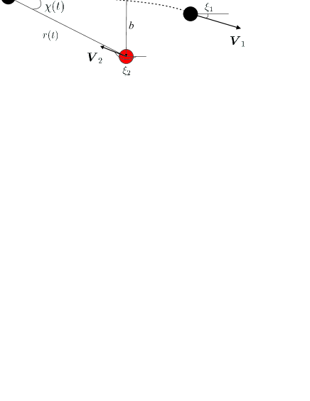
Figure 1: The encounter between a test particle (black) and a background particle (shaded, red online). The interaction causes a small change of the velocity of both particles.

The conservation of momentum before and after the encounter yields

$$mV_{0} = mV_{1}\cos\xi_{1}+MV_{2}\cos\xi_{2}$$ (15)

$$0 =mV_{1}\sin\xi_{1}+MV_{2}\sin\xi_{2}$$

and from the conservation of energy we obtain

$$mV_{0}^{2}=mV_{1}^{2}+MV_{2}^{2}\ .$$ (16)

This enables us to write an equation for $V_{1}$:

$$V_{1}^{2}(m+M)-2mV_{0}V_{1}\cos\xi_{1}+V_{0}^{2}(m-M)=0\ .$$ (17)

We assume that the encounter induces only a small change of the direction of motion of the test particle, so that $\xi_{1}$ can be taken as being small. In this approximation the solution of equation (17) is

$$V_{1}=V_{0}(1-\alpha\xi_{1}^{2})+O(\xi_{1}^{4})$$ (18)

where $\alpha=m/(2M)$. We substitute $V_{1}$ from (18) into equation (III) and obtain

$$\Delta v^{\prime}_{\parallel} \sim -V_{0}\beta\xi_{1}^{2}$$

$$\Delta v^{\prime}_{\perp} \sim V_{0}\xi_{1}$$ (19)

where $\beta=\alpha+1/2=(m+M)/2M$. In the small-angle approximation $\xi_{1}$ is defined by the change of the momentum in the perpendicular direction, so that $\xi_{1}\sim\Delta p_{\perp}/(mV_{0})$. The change of the momentum $\Delta p_{\perp}$ is determined by the force of interaction between particles separated by distance $r$ with magnitude $f(r)=-{\rm d}U(r)/{\rm d}r$, so that $\Delta p_{\perp}$ can be written as

$$\Delta p_{\perp}=-\int_{-\infty}^{\infty}{\rm d}t\frac{{\rm d}U}{{\rm d}r}[r(t)]\sin\chi(t)$$ (20)

where $r(t)$ is a distance between the particles and $\chi(t)$ is an angle between $\mbox{\boldmath$V$}_{0}$ and the vector connecting the particles. We define an impact parameter $b$ to be the initial distance between the test and background particles along the axis perpendicular to $\mbox{\boldmath$V$}_{0}$. From figure 1 we find that $r(t)=\sqrt{x(t)^{2}+b^{2}}$ and $\sin\chi(t)=b/\sqrt{x(t)^{2}+b^{2}}$, where $x(t)$ is a coordinate of the test particle along the direction parallel to $\mbox{\boldmath$V$}_{0}$. Changing the variable $x(t)=V_{0}t$, in the weak-scattering limit where the deflection is small we obtain

$$\Delta p_{\perp}\approx-\frac{1}{V_{0}}\int_{-\infty}^{\infty}{\rm d}x\ \frac{{\rm d}U}{{\rm d}r}(\sqrt{x^{2}+b^{2}})\frac{b}{\sqrt{x^{2}+b^{2}}}\ .$$ (21)

If we denote an integral

$$I(b)=-\int_{-\infty}^{\infty}{\rm d}x\ \frac{{\rm d}U}{{\rm d}r}(\sqrt{x^{2}+b^{2}})\frac{b}{\sqrt{b^{2}+x^{2}}}$$ (22)

we obtain

$$\xi_{1}(b,V_{0})\sim\frac{I(b)}{mV_{0}^{2}}\ .$$ (23)

Using this relation we find

$$\Delta v^{\prime}_{\parallel} = -\frac{\beta I^{2}(b)}{m^{2}V_{0}^{3}}$$

$$\Delta v^{\prime}_{\perp} = \frac{I(b)}{mV_{0}}\ .$$ (24)

Thus, the contribution to the change of the velocity of the test particle due to a single encounter is proportional to $V_{0}^{-3}$ and $V_{0}^{-1}$ in the directions parallel and perpendicular to $\mbox{\boldmath$V$}_{0}$, respectively. Averaging over collisions with many particles is expected to add another factor of $V_{0}$, as the particle propagates with this velocity (see also the derivation below). This suggests that the second moments of the change of the velocity scale as $V_{0}^{-5}$ and $V_{0}^{-1}$ in the directions parallel and perpendicular to $\mbox{\boldmath$V$}_{0}$, respectively. While the latter result is consistent with the behaviour of the diffusion coefficient in the generalised Ornstein-Uhlenbeck process, the former result is different, as in the previous model the result is $\langle\Delta v^{2}_{\parallel}\rangle\sim v^{-3}$. However, if the background particles are not stationary, these estimates must be corrected, as shown below.

We assume that the background particle moves with velocity $\mbox{\boldmath$v$}_{b}$, in which case the discussion above is valid if $\mbox{\boldmath$V$}_{0}$ is a relative velocity of the test particle in the frame of reference moving with the background particle. The velocity of the test particle in a fixed frame of reference is therefore $\mbox{\boldmath$v$}_{0}=\mbox{\boldmath$V$}_{0}+\mbox{\boldmath$v$}_{b}$. We are interested in the changes of the velocity of the test particle in the directions parallel and perpendicular to $\mbox{\boldmath$v$}_{0}$. We denote these $\Delta v_{\parallel}$ and $\Delta v_{\perp}$ and deduce from figure 2:

$$\Delta v_{\parallel} = \Delta v^{\prime}_{\parallel}\cos\Omega+\Delta v^{\prime}_{\perp}\sin\Omega,$$

$$\Delta v_{\perp} = \Delta v^{\prime}_{\perp}\cos\Omega-\Delta v^{\prime}_{\parallel}\sin\Omega$$ (25)

where $\Omega$ is an angle between $\mbox{\boldmath$V$}_{0}$ and $\mbox{\boldmath$v$}_{0}$. These relations are equivalent to the rotation of the coordinate system by angle $\Omega$. Assuming that $v_{0}\gg v_{b}$, where $v_{b}=|\mbox{\boldmath$v$}_{b}|$ and $v_{0}=|\mbox{\boldmath$v$}_{0}|$, we obtain

$$\Omega\sim\frac{\mbox{\boldmath$v$}_{b}\wedge\mbox{\boldmath$V$}_{0}}{V_{0}^{2}}\equiv\frac{v_{b\perp}}{V_{0}}$$ (26)

and $v_{0}\sim V_{0}$. In this approximation, to the leading order in $v_{0}$, we have

$$\Delta v_{\parallel} \approx \frac{I(b)v_{b\perp}}{mv_{0}^{2}}$$

$$\Delta v_{\perp} \approx \frac{I(b)}{mv_{0}}\ .$$ (27)

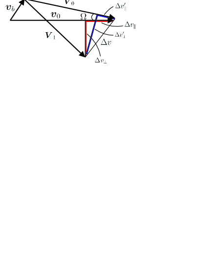
Figure 2: Geometrical construction illustrating the changes of the velocity of the test particle $\Delta v$ parallel and perpendicular to the relative velocity $\mbox{\boldmath$V$}_{0}$ ($\Delta v^{\prime}_{\parallel}$ and $\Delta v^{\prime}_{\perp}$, solid lines, blue online) and the velocity of the test particle $\mbox{\boldmath$v$}_{0}$ ($\Delta v_{\parallel}$ and $\Delta v_{\perp}$, solid lines, red online).

We now imagine that the test particle is travelling through an infinite homogenous population of the background particles with the spatial density number $n$ (measuring a number of particles per unit area) and the probability density of the velocity is $f(\mbox{\boldmath$v$}_{b})$. Let ${\rm d}N$ be the number of background particles it encounters in time $\Delta t$ with velocity $\mbox{\boldmath$v$}_{b}$ in a volume element of velocity space ${\rm d}\mbox{\boldmath$v$}_{b}$ and impact parameter between $b$ and $b+{\rm d}b$. This is the number of particles in two thin stripes, each of width ${\rm d}b$ and length equal to the distance travelled by the particle in $\Delta t$, multiply by the probability $f(\mbox{\boldmath$v$}_{b})\,{\rm d}\mbox{\boldmath$v$}_{b}$. We have

$${\rm d}N\sim 2nV_{0}\Delta t\,{\rm d}b\times f(\mbox{\boldmath$v$}_{b})\,{\rm d}\mbox{\boldmath$v$}_{b}\ .$$ (28)

In order to obtain the total contribution of many background particles with different impact parameters and velocities, we integrate over $b$ and $\mbox{\boldmath$v$}_{b}$,

$$\frac{\langle\Delta v_{\parallel}^{2}\rangle}{2\Delta t} = \frac{n}{m^{2}v_{0}^{3}}\int_{0}^{\infty}{\rm d}b\ I^{2}(b)\int{\rm d}\mbox{\boldmath$v$}_{b}\ f(\mbox{\boldmath$v$}_{b})|\mbox{\boldmath$v$}_{b\perp}|^{2}$$

$$\frac{\langle\Delta v_{\perp}^{2}\rangle}{2\Delta t} = \frac{n}{m^{2}v_{0}}\int_{0}^{\infty}{\rm d}b\ I^{2}(b)\ .$$ (29)

Here we used the assumption that $U(r)$ is a short-ranged, allowing us to let the upper limit of the integral over $b$ approach infinity. In the case of the original Chandrasekhar-Rosenbluth model, an upper limit to the impact parameter must be introduced because of the long-range interaction between the particles. This leads to logarithmic correction terms Cha43 ; Ros+57 .

Equations (III), describing the velocity increments for the Chandrasekhar-Rosenbluth model has the same scaling (as a function of $v_{0}$) as scaling of the diffusion coefficients for the generalised Ornstein-Uhlenbeck model (as a function of $p$; see equations (12) and (13)). This indicates that the anomalous diffusion behaviour of these models is equivalent.

IV Probability density function and moments of the momentum

Now we return to the generalised Ornstein-Uhlenbeck process and obtain the closed-form solution of the Fokker-Planck equation for a particular choice of the initial conditions. We use this solution to obtain an exact expression for the growth of the moments of the momentum.

We first consider the two-dimensional case. The probability density for the momentum satisfies equation (11), with the diffusion coefficients given by (12) and (13). We transform to polar coordinates and seek a probability density $P(p,\theta,t)$, and consider the case when the particle is initially at rest, so that the initial condition is $P(p,\theta,0)=\delta(p)$. This circularly symmetric solution, $P=\rho(p,t)$, satisfies

$$\frac{\partial\rho}{\partial t}=\frac{D_{3}p_{0}^{3}}{p^{3}}\frac{\partial^{2}\rho}{\partial p^{2}}+\left(\gamma p-\frac{2D_{3}p_{0}^{3}}{p^{4}}\right)\frac{\partial\rho}{\partial p}+2\gamma\rho\ .$$ (30)

By analogy with the solution of the one-dimensional generalised Ornstein-Uhlenbeck model, we find the following normalised closed-form solution of (30):

$$\rho(p,t) = \frac{5}{\Gamma(2/5)}\frac{\gamma^{2/5}}{[5D_{3}p_{0}^{3}(1-{\rm e}^{-5\gamma t})]^{2/5}}$$ (31)

$$\times {\rm exp}\left[-\frac{\gamma p^{5}}{5D_{3}p_{0}^{3}(1-{\rm e}^{-5\gamma t})}\right]\ .$$

In the long-time limit the density is non-Maxwellian given by

$$\rho_{0}(p)=\frac{5\gamma^{2/5}}{\Gamma(2/5)(5D_{3}p_{0}^{3})^{2/5}}{\rm exp}\left[-\frac{\gamma p^{5}}{5D_{3}p_{0}^{3}}\right]\ .$$ (32)

Using the probability density (31) we determine the $l$-th moment of $p$,

$$\langle p^{l}(t)\rangle = \int_{0}^{\infty}{\rm d}p\ p^{l+1}\rho(p,t)$$ (33)

$$= \left(\frac{5D_{3}p_{0}^{3}}{\gamma}\right)^{l/5}\frac{\Gamma[(2+l)/5]}{\Gamma(2/5)}(1-{\rm e}^{-5\gamma t})^{l/5}\ .$$

We remark that an additional factor of $p$ in the expression above appears as a weight in the transformation to polar coordinates.

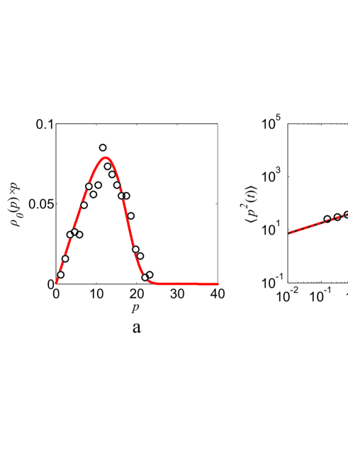
Figure 3: Shows results of the numerical simulation of equation (1) for the motion in the two-dimensional potential force field. Panel a shows stationary non-Maxwellian density function (32) (solid line) and data from the numerical simulation (circles). Panel b shows the second moment of the momentum (33) with $l=2$ (solid line) and data from the numerical simulation (circles). The dashed line shows the slope $t^{2/5}$ and dotted line indicates time $\gamma^{-1}$ at which the density becomes stationary. The results are for the case of a Gaussian correlation function of the potential $C(x,t)=\sigma^{2}{\rm exp}[-x^{2}/(2\eta^{2})-t^{2}/(2\tau^{2})]$ with $\sigma=15$, $\tau=0.1$ and $\eta=0.1$. The other parameters were $m=1$ and $\gamma=0.01$.

In the three-dimensional case we find a similar solution to equation (10) in the case where the particles are initially stationary. We write this equation in spherical polar coordinates, and seek a spherically symmetric solution, $P(p,\theta,\phi,t)=\rho(p,t)$. The solution of the corresponding equation for $\rho(p,t)$ is obtained similarly to the two-dimensional case and we have

$$\rho(p,t) = \frac{5}{\Gamma(3/5)}\frac{\gamma^{3/5}}{[5D_{3}p_{0}^{3}(1-{\rm e}^{-5\gamma t})]^{3/5}}$$ (34)

$$\times {\rm exp}\left[-\frac{\gamma p^{5}}{5D_{3}p_{0}^{3}(1-{\rm e}^{-5\gamma t})}\right].$$

This determines moments of the momentum

$$\langle p^{l}(t)\rangle = \left(\frac{5D_{3}p_{0}^{3}}{\gamma}\right)^{l/5}\frac{\Gamma[(3+l)/5]}{\Gamma(3/5)}$$ (35)

$$\times (1-{\rm e}^{-5\gamma t})^{l/5}\ .$$

For both two- and three-dimensional cases we obtain that at short times the variance of the momentum grows as

$$\langle p^{2}(t)\rangle\sim t^{2/5}\ .$$ (36)

Thus, at short times the momentum diffuses anomalously with the same exponent as in the one-dimensional model Gol+91 ; Ros92 . The results for the stationary probability density and diffusion of the momentum in the two-dimensional case were verified by a numerical simulation, documented in figure 3.

V Spatial diffusion

In this section we find the mean-square value of the displacement of a particle which starts at the origin:

$$\langle|\mbox{\boldmath$x$}(t)|^{2}\rangle = \frac{1}{m^{2}}\int_{0}^{t}dt_{1}\int_{0}^{t}dt_{2}\ \langle\mbox{\boldmath$p$}(t_{1})\cdot\mbox{\boldmath$p$}(t_{2})\rangle$$ (37)

$$= \frac{1}{m^{2}}\int_{0}^{t}dt_{1}\int_{0}^{t}dt_{2}\ \langle p(t_{1})p(t_{2})\cos\theta\rangle$$

where $\theta$ is an angle between $\mbox{\boldmath$p$}(t_{1})$ and $\mbox{\boldmath$p$}(t_{2})$. We recall that when the force is the gradient of the potential, we have $D_{xx}\lll D_{yy}$ for $p\gg p_{0}$ implying that the correlation of the angle vanishes much more rapidly than the correlation of the magnitude of the momentum. We can, therefore, perform the averaging in (37) by first integrating over the correlation function of the angular variable, with the momentum held fixed, and then finally performing the averaging over fluctuations of the momentum.

In the two-dimensional case the probability density $P(\theta,t)$ of $\theta$ satisfies the diffusion equation on a circle with the initial condition $P(\theta,0)=\delta(\theta)$. The solution is Gaussian:

$$P(\theta,t) = \frac{1}{2\sqrt{\pi\mathcal{D}t}}$$ (38)

$$\times {\rm exp}\left(-\frac{\theta^{2}}{4\mathcal{D}t}\right),$$

where $\mathcal{D}=D_{1}p_{0}/p^{3}(t_{1})$. Using this probability density we calculate the expectation value

$$\langle\cos\theta\rangle={\rm exp}\left(-\mathcal{D}|t_{2}-t_{1}|\right).$$ (39)

We thus obtain from equations (37) and (39)

$$\langle|\mbox{\boldmath$x$}(t)|^{2}\rangle \sim \frac{1}{m^{2}}\int_{0}^{t}{\rm d}t_{1}\int_{0}^{t}{\rm d}t_{2}\int_{0}^{\infty}{\rm d}p\ \rho(p,t_{1})p^{3}(t_{1})$$ (40)

$$\times {\rm exp}\left(-\mathcal{D}|t_{2}-t_{1}|\right).$$

Introducing a new variable $T=t_{1}-t_{2}$ we have

$$\langle|\mbox{\boldmath$x$}(t)|^{2}\rangle \sim \frac{2}{m^{2}}\int_{0}^{t}{\rm d}t_{1}\int_{0}^{t}{\rm d}T$$ (41)

$$\times \int_{0}^{\infty}{\rm d}p\ \rho(p,t_{1})p^{3}(t_{1}){\rm exp}\left(-\frac{D_{1}p_{0}}{p^{3}(t_{1})}T\right)$$

$$= \frac{2}{m^{2}D_{1}p_{0}}\int_{0}^{t}{\rm d}t_{1}\int_{0}^{\infty}{\rm d}p\ \rho(p,t_{1})p^{6}(t_{1})$$

$$\times \left[1-{\rm exp}\left(-\frac{D_{1}p_{0}}{p^{3}(t_{1})}t\right)\right]\ .$$

When the forcing is strong we have $D_{1}p_{0}t\gg p^{3}$ for $t\gg\tau$, and therefore

$$\langle|\mbox{\boldmath$x$}(t)|^{2}\rangle = \frac{2}{m^{2}D_{1}p_{0}}\int_{0}^{t}{\rm d}t_{1}\int_{0}^{\infty}{\rm d}p\ \rho(p,t_{1})p^{6}(t_{1})$$ (42)

$$= \frac{2}{m^{2}D_{1}p_{0}}\int_{0}^{t}{\rm d}t_{1}\langle p^{5}(t_{1})\rangle\ .$$

Using equation (33) we obtain

$$\langle|\mbox{\boldmath$x$}(t)|^{2}\rangle=\frac{4D_{3}p_{0}^{2}}{5D_{1}m^{2}\gamma^{2}}(5\gamma t+{\rm e}^{-5\gamma t}-1)\ .$$ (43)

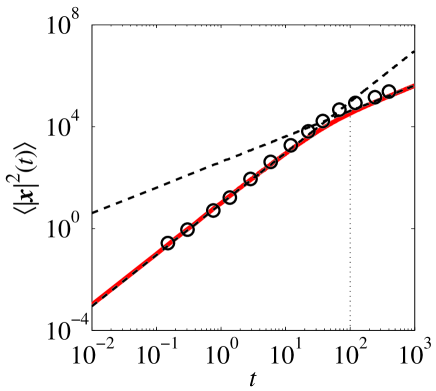
Figure 4: Shows results for the spatial diffusion in the two-dimensional potential force-field. The results from the numerical simulation (circles) are compared with equation (43) (solid line). Dashed lines show the slopes $t^{2}$ and $t$ and dotted line indicates the time $\gamma^{-1}$. The parameters of the simulation are the same as in figure 3.

In the three-dimensional case the probability density of $\cos\theta$ can be found by considering the diffusion equation on a spherical surface, with polar coordinates $(\theta,\phi)$, starting from the pole, $\theta=0$. The solution $P(\theta,\phi,t)$ of the diffusion equation may be expressed as a linear combination of spherical harmonics. Because the problem has a rotational symmetry, the solution is independent of the azimuthal angle $\phi$, and it may be written as:

$$P(\theta,\phi,t)=\sum_{l=0}^{\infty}A_{l}\ {\rm exp}\left[-\frac{l(l+1)p_{0}D_{1}}{p^{3}}t\right]P_{l}(\cos\theta)$$ (44)

where $P_{l}(z)$ is a Legendre polynomial of degree $l$. Using the orthogonality relations for Legendre polynomials, in view of the initial condition $\cos\theta=1$, we obtain $A_{l}=(2l+1)/2$. Also, the quantity that we wish to average is itself a spherical harmonic: $\cos\theta=P_{1}(\cos\theta)$, so that only the $l=1$ term in (44) contributes to the correlation function. Hence we obtain

$$\langle\cos\theta(|t_{2}-t_{1}|)\rangle={\rm exp}\left(-3\mathcal{D}|t_{2}-t_{1}|\right),$$ (45)

where $\mathcal{D}=p_{0}D_{1}/p^{3}$ is the same as in the two-dimensional case. Using this angular correlation function we calculate

$$\langle|\mbox{\boldmath$x$}(t)|^{2}\rangle \sim \frac{1}{m^{2}}\int_{0}^{t}{\rm d}t_{1}\int_{0}^{t}{\rm d}t_{2}\int_{0}^{\infty}{\rm d}p\ \rho(p,t_{1})p^{4}(t_{1})$$ (46)

$$\times {\rm exp}\left(-3\mathcal{D}|t_{2}-t_{1}|\right).$$

The evaluation of the integral using the probability density (35) yields

$$\langle|\mbox{\boldmath$x$}(t)|^{2}\rangle=\frac{2D_{3}p_{0}^{2}}{5D_{1}m^{2}\gamma^{2}}(5\gamma t+{\rm e}^{-5\gamma t}-1).$$ (47)

We find that in two- and three-dimensional cases $\langle|\mbox{\boldmath$x$}(t)|^{2}\rangle\sim t^{2}$ at short times, so that the particle diffuses ballistically. The results are consistent with a short-time asymptotic behaviour of the undamped particle obtained in Ros92 for $d>1$. The long-time behaviour is naturally diffusive, $\langle|\mbox{\boldmath$x$}(t)|^{2}\rangle\sim t$. In Fig. 4 we show the comparison of the analytical and numerical results for $\langle|\mbox{\boldmath$x$}(t)|^{2}\rangle$ for the case of motion in the two-dimensional potential force field, illustrating the short-time ballistic diffusion.

VI Summary

We have investigated generalizations of two classical models for diffusion of a particle accelerated by random forces. We discussed a generalization of the classical Ornstein-Uhlenbeck process where the force depends on the position of the particle as well as time. We also modified the Chandrasekhar-Rosenbluth model by considering motion due to a short-range interaction potential. Although both models are described by different microscopic equations of motion, surprisingly, they have the same scaling of the diffusion coefficients, leading to the same short-time asymptotic dynamics.

We solved the Fokker-Planck equation for the generalised Ornstein-Uhlenbeck process exactly in two and three dimensions, building upon our earlier analysis of the one-dimensional case in Arv+05 ; Bez+06 . We have shown that this dynamics is characterised by anomalous diffusion of the momentum, with the variance which scales as $\langle p^{2}\rangle\sim t^{2/5}$. At long time, the distribution of the momentum has been found to be non-Maxwellian. The second moment of the displacement grows ballistically at short times, that is $\langle x^{2}\rangle\sim t^{2}$, in accord with a surmise made by Rosenbluth for a closely related model Ros92 , and at long time a simple diffusive behaviour of the displacement is recovered.

References

• (1) R. Metzler and J. Klafter, Phys. Rep., 339, 1, (2000).
• (2) L. S. Uhlenbeck and G. E. Ornstein, Phys. Rev., 36, 823, (1930)- CHECK.
• (3) E. Arvedson, B. Mehlig, M. Wilkinson, and K. Nakamura, Phys. Rev. Lett., 96, 030601, (2006).
• (4) V. Bezuglyy, B. Mehlig, M. Wilkinson, K. Nakamura, and E. Arvedson, J. Math. Phys., 47, 073301, (2006).
• (5) L. Golubovic, S. Feng, and F.-A. Zeng, Phys. Rev. Lett., 67, 2115 (1991).
• (6) M. N. Rosenbluth, Phys. Rev. Lett., 69, 1831, (1992).
• (7) S. Chandrasekhar, Astrophys. J., 97, 255, (1992).
• (8) M. N. Rosenbluth, W. M. MacDonald and D. L. Judd, Phys. Rev. 107, 1 (1957).
• (9) P. A. Sturrock, Phys. Rev., 141, 186, (1966).
• (10) B. Aguer, S. de BiΓ¨vre, P. Lafitte and P. E. Parris, J. Stat. Phys., 138, 780-814, (2010).
• (11) J. Binney and S. Tremaine, Galactic dynamics, Princenton University Press (1994)