Asymptotic Total Variation Tests for Copulas

JEAN-DAVID FERMANIAN, DRAGAN RADULOVIĆ and MARTEN WEGKAMP

t2The research of Wegkamp is supported in part by NSF DMS 1007444 and NSF DMS 1310119 grants.

Jean-David Fermanian
Crest-Ensae
3 av. Pierre Larousse
92245 Malakoff cedex, France
E-mail: jean-david.fermanian@ensae.fr

Dragan Radulović
Department of Mathematics
Florida Atlantic University, USA
E-mail: radulovi@fau.edu

Marten Wegkamp
Department of Mathematics & Department of Statistical Science
Cornell University, USA
E-mail: marten.wegkamp@cornell.edu

We propose a new platform of goodness-of-fit tests for copulas, based on empirical copula processes and nonparametric bootstrap counterparts. The standard Kolmogorov-Smirnov type test for copulas that takes the supremum of the empirical copula process indexed by orthants is extended by test statistics based on the empirical copula process indexed by families of $L_{n}$ disjoint boxes, with $L_{n}$ slowly tending to infinity. Although the underlying empirical process does not converge, the critical values of our new test statistics can be consistently estimated by nonparametric bootstrap techniques, under simple or composite null assumptions. We implemented a particular example of these tests and our simulations confirm that the power of the new procedure is oftentimes higher than the power of the standard Kolmogorov-Smirnov or the Cramér-von Mises tests for copulas.

AMS 2000 subject classifications: Primary 60F17, 60K35; secondary 60G99.

Keywords: Bootstrap, copula, empirical copula process, goodness-of-fit Test, weak Convergence.

1 Introduction

This paper introduces new powerful goodness-of-fit (GOF) tests for copulas in $[0,1]^{d}$, $d\geq 2$, based on the empirical copula process

$$\mathbb{Z}_{n}(\mathbf{u})=\sqrt{n}(\mathbb{C}_{n}-C)(\mathbf{u}),\qquad\mathbf{u}=(u_{1},\ldots,u_{d})\in[0,1]^{d},$$ (1.1)

given a sample of $n$ independent random vectors $\mathbf{X}_{i}=(X_{i1},\ldots,X_{id})\in\mathbb{R}^{d}$, $i=1,\ldots,n$, from a common distribution function $H$. Let $C$ be the associated copula function, as given by Sklar’s Theorem (Sklar, 1959). Here $\mathbb{C}_{n}$ is the usual empirical copula, as introduced by Deheuvels (1979): denoting by $\mathbb{H}_{n}$ the joint cdf of the sample $(\mathbf{X}_{1},\ldots,\mathbf{X}_{n})$, $\mathbb{F}_{n,j}$ the $j$-th empirical cdf associated to $(X_{1j},\ldots,X_{nj})$, $j=1,\ldots,d$, and $\mathbb{F}_{n,j}^{-}$ its empirical quantile function, we have

$$\mathbb{C}_{n}(\mathbf{u})=\mathbb{H}_{n}(\mathbb{F}_{n,1}^{-}(u_{1}),\ldots,\mathbb{F}_{n,d}^{-}(u_{d}))$$

by definition, for every $\mathbf{u}=(u_{1},\ldots,u_{d})\in[0,1]^{d}$. The Kolmogorov-Smirnov (KS) test statistic for testing of the null hypothesis $\mbox{$\rm H$}_{0}:\,C=C_{0}$ is

$${\rm KS}_{n}=\sup_{\mathbf{u}\in[0,1]^{d}}|\sqrt{n}(\mathbb{C}_{n}-C_{0})(\mathbf{u})|.$$ (1.2)

The Cramér-von Mises statistic (CvM) is

$${\rm CM}_{n}=\int\{\sqrt{n}(\mathbb{C}_{n}-C_{0})(\mathbf{u})\}^{2}\,{\rm d}\mathbb{C}_{n}(\mathbf{u}).$$ (1.3)

It is well-known, see, for instance, Fermanian et al. (2004), that $\mathbb{Z}_{n}$ and its bootstrap counterpart $\mathbb{Z}_{n}^{*}$, defined in (2.4) below, both converge weakly to the same tight Gaussian process in $\ell^{\infty}([0,1]^{d})$ under the null hypothesis. Therefore, we can compute the $\alpha$-upper points of ${\rm KS}_{n}$ and ${\rm CM}_{n}$ via the bootstrap. To the best of our knowledge, all the proposed GOF tests rely on simulation-based procedures to calculate their corresponding p-values, with the notable exception of the distribution-free test statistics of Fermanian (2005). The latter idea has been further developed by Scaillet (2007) and Fermanian and Wegkamp (2012). A parametric bootstrap has been proposed (Genest and Rémillard, 2008) to tackle composite null hypotheses, while Rémillard and Scaillet (2009) advocate the use of the multiplier central limit theorem to build an alternative bootstrap empirical copula process. Bücher and Dette (2010) give a survey and a comparison of various bootstrap methods.

The goal of this paper is to develop more powerful tests than the KS test (1.2) and CvM test (1.3) for simple and composite null hypotheses. The next section offers a class of such tests. For instance, in the case of a null simple hypothesis $\mbox{$\rm H$}_{0}:\,C=C_{0}$, we propose the test that rejects $\mbox{$\rm H$}_{0}$ for large values of the test statistic

$$\mathbb{T}_{n}:=\sup_{B_{1},\ldots,B_{L_{n}}}\sum_{k=1}^{L_{n}}|\mathbb{Z}_{n}(B_{k})|.$$ (1.4)

The supremum is taken over all disjoint boxes $B_{1},\ldots,B_{L_{n}}\subset[0,1]^{d}$ of the form $\prod_{j=1}^{d}(a_{j},b_{j}]$, using the convention

$$\mathbb{Z}_{n}((a_{1},b_{1}]\times\cdots\times(a_{d},b_{d}])=\Delta_{a_{1},b_{1}}^{1}\Delta_{a_{2},b_{2}}^{2}\cdots\Delta_{a_{d},b_{d}}^{d}\mathbb{Z}_{n}(\mathbf{u}),$$ (1.5)

for any arbitrary point $\mathbf{u}\in[0,1]^{d}$ and for all $0\leq a_{j}<b_{j}\leq 1$, $j=1,\ldots,d$. Here, we have used the usual operators $\Delta^{j}$ defined for every function $f$ by

$$\left(\Delta^{j}_{a,b}f\right)(\mathbf{u})=f(u_{1},\ldots,u_{j-1},b,u_{j+1},\ldots,u_{d})-f(u_{1},\ldots,u_{j-1},a,u_{j+1},\ldots,u_{d}),$$

for all $\mathbf{u}\in[0,1]^{d}$, and all real numbers $a$ and $b$.

We will also consider the related statistics

$$\widetilde{\mathbb{T}}_{n}=\max_{B_{1},...,B_{L_{n}}}\sum_{i=1}^{L_{n}}|\mathbb{Z}_{n}(B_{i})|\text{ ,\ }$$ (1.6)

with the maximum taken over all disjoint rectangles $B_{1},...,B_{L_{n}}$ of the form $B=\Pi_{j=1}^{d}(a_{j},b_{j}]$ with $a_{j},b_{j}$ belonging to a grid $\{{n^{-1/d}},{2}{n^{-1/d}},\ldots,{\lfloor n^{1/d}\rfloor}{n^{-1/d}}\}.$ Asymptotically, $\widetilde{\mathbb{T}}_{n}$ and $\mathbb{T}_{n}$ are the same (since $|\widetilde{\mathbb{T}}_{n}-\mathbb{T}_{n}|=o_{p}(1)$ by Lemma 9 and Proposition 10 in Section 5), but $\widetilde{\mathbb{T}}_{n}$ is computationally much more tractable.

Now, if $L_{n}=L$ for all $n$, the collection of boxes is sufficiently small that we can still appeal to the weak convergence of $\mathbb{Z}_{n}$ and $\mathbb{Z}_{n}^{*}$ in conjunction with the continuous mapping theorem, to obtain $\alpha$-upper points of the test statistic $\mathbb{T}_{n}$ via the bootstrap. Taking $L_{n}=+\infty$ for all $n$, or equivalently, if we consider all families of disjoint boxes in $[0,1]^{d}$ (possibly partitions), the statistic $\mathbb{T}_{n}$ is equal to the total variation distance $TV(\mathbb{Z}_{n})$ of $\mathbb{Z}_{n}$. The resulting test is not statistically meaningful as $TV(\mathbb{Z}_{n})$ is maximal, to wit, $TV(\mathbb{Z}_{n})=n^{1/2}\rightarrow+\infty$. The problem is to find a rich collection that quickly detects departure from the null, but still yields a consistent test. The main novelty of our approach is the fact that we let $L_{n}$, the number of boxes, slowly tend to $\infty$ in that $L_{n}\sim(\log n)^{\gamma}$, $0<\gamma<1$. While in this case the process $\mathbb{Z}_{n}$ no longer converges, Theorem 1 in Section 2 states that we can still consistently estimate the distribution of the process $\mathbb{Z}_{n}$ by the bootstrap. We refer to our procedure as the Asymptotic Total Variation (ATV) test. The considered families of boxes are finer and finer, presumably improving the power of the test, while for each $n$ large enough, we still have a consistent test in that we control the type 1 error. A key observation is that under the null hypothesis ${\rm H}_{0}:\,C=C_{0}$, we have $\mathbb{T}_{n}\leq L_{n}\sup_{B}|\mathbb{Z}_{n}(B)|=O_{p}(L_{n})$, while under the alternative ${\rm H}_{A}:\,C=C_{1}$ for some fixed $C_{1}\neq C_{0}$, $\mathbb{T}_{n}$ is much larger since the bias is at least of order $O({n^{1/2}})$.

Theorem 1 extends the surprising result obtained by Radulović (2012) for empirical processes indexed by sums of indicator functions of VC-graph classes (see Theorem 13 in the appendix). We require very mild conditions on the copula function $C$. This is one of the few notable exceptions known to us in the literature where the bootstrap “works”, that is, the conditional bootstrap distribution consistently estimates the distribution of the test statistic, while the distribution of the statistic itself does not converge. For other instances of this phenomenon, we refer to Bickel and Freedman (1983) and, more recently, Radulović (1998, 2012, 2013).

Section 3 considers the more general hypothesis that the underlying copula $C$ belongs to some parametric copula family $\{C_{\theta},\,\theta\in\Theta\subset\mathbb{R}^{p}\}$. Given a sufficiently regular estimator $\widehat{\theta}$ and its bootstrap counterpart $\widehat{\theta}^{*}$, we adjust our statistic (1.4) and its non-parametric bootstrap counterpart to obtain a consistent level $\alpha$ test (Theorem 4). Again, the result is established under very mild regularity conditions on the copula $C_{\theta}$ and the estimators $\widehat{\theta}$ and $\widehat{\theta}^{*}$. Incidentally, we introduce a new bootstrap procedure under composite null hypotheses, an alternative to the usual parametric bootstrap or the multiplier CLT.

Section 4 then reports a small numerical study where we show that, in complex but realistic situations, our test (1.4) is superior to the Kolmogorov-Smirnov and the Cramér-von Mises tests. We also comment on a possible inadequacy in the way the copula GOF tests are commonly evaluated. Finally, the proofs are collected in Section 5. The appendix contains some technical results from Segers (2012) and Radulović (2012) and a description of the implementation of the proposed tests.

2 The Asymptotic Total Variation Test

Notations. Let $H$ be the distribution function of the random vector $\mathbf{X}$ with marginals $F_{1},\ldots,F_{d}$. We will assume throughout the paper that $H$ is continuous. Let $(\mathbf{X}_{1},\ldots,\mathbf{X}_{n})$ be independent copies of $\mathbf{X}$. We denote the generalized inverse of a distribution function $F$ by $F^{-}$. For instance, $F_{j}^{-}(u)=\inf\{x\,|\,F_{j}(x)\geq u\}$. The empirical counterparts of $H$ and any $F_{j}$ are, respectively,

$$\mathbb{H}_{n}(\mathbf{x}) = \frac{1}{n}\sum_{i=1}^{n}\mathbf{1}\{\mathbf{X}_{i}\leq\mathbf{x}\},\ \mathbf{x}\in\mathbb{R}^{d}$$

$$\mathbb{F}_{n,j}(x) = \frac{1}{n}\sum_{i=1}^{n}\mathbf{1}\{X_{i,j}\leq x\},\ x\in\mathbb{R},\ \;j=1,\ldots,d.$$

The copula function of $\mathbf{X}$ is $C(\mathbf{u})=H(F_{1}^{-}(u_{1}),\ldots,F_{d}^{-}(u_{d}))$, $\mathbf{u}=(u_{1},\ldots,u_{d})\in[0,1]^{d}$, and its empirical estimate is $\mathbb{C}_{n}(\mathbf{u})=\mathbb{H}_{n}(\mathbb{F}_{n,1}^{-}(u_{1}),\ldots,\mathbb{F}_{n,d}^{-}(u_{d}))$. The empirical copula process $\mathbb{Z}_{n}(\mathbf{u})=\sqrt{n}(\mathbb{C}_{n}-C)(\mathbf{u})$ is already defined in (1.1). We define $\mathcal{F}_{n}$ as the class of functions

$$f(\mathbf{x})=\sum_{k=1}^{L_{n}}c_{k}\mathbf{1}\{\mathbf{x}\in B_{k}\},$$ (2.1)

with $c_{k}\in\{-1,+1\}$ and disjoint boxes $B_{k}$ of the form $\prod_{j=1}^{d}(a_{j},b_{j}]$ in the unit cube $[0,1]^{d}$, for all $1\leq k\leq L_{n}$. We let

$$\mathbb{Z}_{n}(f)=\sum_{k=1}^{L_{n}}c_{k}\mathbb{Z}_{n}(B_{k}),$$

and observe that

$$\mathbb{T}_{n}=\sup_{f\in\mbox{$\mathcal{F}_{n}$}}|\mathbb{Z}_{n}(f)|=\sup_{B_{1},\ldots,B_{L_{n}}}\sum_{k=1}^{L_{n}}|\mathbb{Z}_{n}(B_{k})|,$$

where the supremum is taken over all disjoint boxes $B_{1},\ldots,B_{L_{n}}$ of the unit square $[0,1]^{d}$.

If $L_{n}=L$ for all $n$, then $\mbox{$\mathcal{F}$}_{n}=\mbox{$\mathcal{F}$}$ and $\mathbb{Z}_{n}$ converges in $\ell^{\infty}(\mbox{$\mathcal{F}$})$ to a Gaussian process under regularity conditions on $C$, see, for instance, Fermanian et al. (2004) and Segers (2012). As a consequence of the continuous mapping theorem, $\mathbb{T}_{n}$ trivially converges weakly as well. However, if $L_{n}\rightarrow\infty$, as $n\rightarrow\infty$, this is no longer true as the process $\mathbb{Z}_{n}$ does not converge weakly.

The main point of this paper is to show that, provided $L_{n}=(\log n)^{\gamma}$ for some $0<\gamma<1$, the distribution of $\mathbb{T}_{n}$ can be estimated by the bootstrap. The bootstrap counterparts of the above processes are defined as follows. Let the bootstrap sample $(\mathbf{X}_{1}^{*},\ldots,\mathbf{X}_{n}^{*})$ be obtained by sampling with replacement from $\mathbf{X}_{1}$,$\ldots$, $\mathbf{X}_{n}$. We write

$$\mathbb{H}_{n}^{*}(\mathbf{x})=\frac{1}{n}\sum_{i=1}^{n}\mathbf{1}\{\mathbf{X}_{i}^{*}\leq\mathbf{x}\},\ \mathbf{x}\in\mathbb{R}^{d},$$ (2.2)

for the empirical cdf based on the bootstrap, with marginals

$$\mathbb{F}_{n,j}^{*}(x)=\frac{1}{n}\sum_{i=1}^{n}\mathbf{1}\{X_{i,j}^{*}\leq x\},\ x\in\mathbb{R},\ j=1,\ldots,d.$$ (2.3)

We denote its associated empirical copula function by $\mathbb{C}_{n}^{*}$. The bootstrap empirical copula process is

$$\mathbb{Z}_{n}^{*}=\sqrt{n}(\mathbb{C}_{n}^{*}-\mathbb{C}_{n})=\sqrt{n}\left\{\mathbb{H}_{n}^{*}(\mathbb{F}_{n,1}^{*-},\ldots,\mathbb{F}_{n,d}^{*-})-\mathbb{H}_{n}(\mathbb{F}_{n,1}^{-},\ldots,\mathbb{F}_{n,d}^{-})\right\}.$$ (2.4)

Assumptions. We will assume the following set of assumptions:

• For any $j=1,\ldots,d$, for all $\mathbf{u}\in[0,1]^{d}$ with $0<u_{j}<1$, the first-order partial derivative $C_{j}(\mathbf{u})=\partial C(\mathbf{u})/\partial u_{j}$ exists and is of bounded variation (Hildebrandt, 1963, e.g.). Moreover, it satisfies, for some $r>0$, $\beta\geq 0$ and $K<\infty$,

  $$|C_{j}(\mathbf{u})-C_{j}(\mathbf{v})|\leq K\left(u_{j}^{-\beta}(1-u_{j})^{-\beta}+v_{j}^{-\beta}(1-v_{j})^{-\beta}\right)\sum_{l=1}^{d}|u_{l}-v_{l}|^{r},$$

  for all $\mathbf{u},\mathbf{v}\in[0,1]^{d}$, $0<u_{j},v_{j}<1$. As in Segers (2013), we extend the domain of each $C_{j}$ to the whole $[0,1]^{d}$ by setting

  $$C_{j}(\mathbf{u}):=\left\{\begin{array}[]{ll}\limsup_{h\downarrow 0}\frac{C(\mathbf{u}+h{\bf e}_{j})}{h}&\text{ if }\mathbf{u}\in[0,1]^{d},u_{j}=0;\\ \limsup_{h\downarrow 0}\frac{C(\mathbf{u})-C(\mathbf{u}-h{\bf e}_{j})}{h}&\text{ if }\mathbf{u}\in[0,1]^{d},u_{j}=1.\end{array}\right.$$

  Here ${\bf e}_{j}$ is the $j$th coordinate vector in $\mathbb{R}^{d}$.
  

• The number $L_{n}$ is of order $(\log n)^{\gamma}$ for some $0<\gamma<1$.
  

Remark. We know that continuity of the partial derivatives of $C$ on $(0,1)^{d}$ is required for weak convergence, see Fermanian et al. (2004) and Segers (2012). The requirement that the partial derivatives are of bounded variation is natural since we compute the supremum of $\mathbb{Z}_{n}$ over increasingly finer families of boxes in $[0,1]^{d}$. The process $\mathbb{Z}_{n}(\mathbf{u})$ is asymptotically equivalent to $\alpha_{n}(\mathbf{u})-\sum_{j=1}^{d}C_{j}(\mathbf{u})\alpha_{n,j}(u_{j})$ with $\alpha_{n}(\mathbf{u})=\sqrt{n}(\mathbb{H}_{n}-H)(\mathbf{u})$ and $\alpha_{n,j}(u_{j})=\sqrt{n}(\mathbb{F}_{n,j}-F)(u_{j})$ (see Proposition 10).

Remark. The additional requirement (C1) is weaker than imposing a Hölder condition on the derivatives. Segers (2012) imposes a slightly stronger condition on the second-order partial derivatives of $C$ (corresponding to $r=1$) to obtain an almost sure representation of the empirical copula process.

Indeed, as a counterexample, consider the bivariate Archimedean copula $C$ whose generator is given by $\psi:(0,1]\rightarrow\mathbb{R}^{+}$, $\psi(t):=\exp(t^{-\theta})-e$ for some $\theta>0$. This copula, see display (4.2.20) in Nelsen (2006), is

$$C(u_{1},u_{2})=\left[\ln\left(\exp(u_{1}^{-\theta})+\exp(u_{2}^{-\theta})-e\right)\right]^{-1/\theta},$$

for any $\mathbf{u}\in[0,1]^{2}$. It can be checked easily that, when $u\rightarrow 0$, the copula density

$$C_{12}(u,u)\sim\frac{\theta^{2}}{4}u^{-\theta-1}.$$

Therefore, $C$ cannot fulfill Condition 4.1 in Segers (2012). Nonetheless, by the mean value theorem and simple calculations, we can prove that

$$|C_{1}(\mathbf{u})-C_{1}(\mathbf{v})|\leq K(\min(u_{1},v_{1}))^{-2\theta-2}|u_{1}-v_{1}|+K(\min(u_{1},v_{1}))^{-\theta-1}|u_{2}-v_{2}|.$$

Since the same reasoning can be done with $C_{2}$, our condition (C1) is fulfilled.

The second assumption (C2) allows for sub-logarithmic rate in the sample size for the number of boxes considered. In practice, even this fairly slow rate yields much better tests, see our simulations in Section 4. And we have not observed any significant differences empirically between choosing $\gamma=1$ and $\gamma$ closed to one.

Our first result states that the processes $\mathbb{Z}_{n}$ and $\mathbb{Z}_{n}^{*}$ are close in the bounded Lipschitz distance that characterizes weak convergence. Formally, we show that

$$\mathbb{E}\left[\sup_{h}\left|\mathbb{E}[h(\mathbb{Z}_{n})]-\mathbb{E}^{*}[h(\mathbb{Z}_{n}^{*})]\right|\right]$$ (2.5)

is asymptotically negligible. Here $\mathbb{E}^{*}$ is the conditional expectation with respect to the bootstrap sample and the supremum in (2.5) is taken over $BL_{1}=BL_{1}(\ell^{\infty}(\mbox{$\mathcal{F}$}_{n}))$, the class of all uniformly bounded, Lipschitz functionals $h:\ell^{\infty}(\mbox{$\mathcal{F}$}_{n})\rightarrow\mathbb{R}$ with Lipschitz constant 1, that is,

$$\sup_{x\in\ell^{\infty}(\mbox{$\mathcal{F}$}_{n})}|h(x)|\leq 1$$ (2.6)

and, for all $x,y\in\ell^{\infty}(\mbox{$\mathcal{F}$}_{n})$,

$$|h(x)-h(y)|\leq\sup_{f\in\mbox{$\mathcal{F}$}_{n}}|x(f)-y(f)|.$$ (2.7)

Theorem 1.

Let $\mathbb{Z}_{n}=\{\mathbb{Z}_{n}(f),\ f\in\mbox{$\mathcal{F}$}_{n}\}$ and $\mathbb{Z}_{n}^{*}=\{\mathbb{Z}_{n}^{*}(f),\ f\in\mbox{$\mathcal{F}$}_{n}\}$ with $\mbox{$\mathcal{F}$}_{n}$ as defined in (2.1) above. Under conditions (C1) and (C2), we have

$$\lim_{n\rightarrow\infty}\mathbb{E}\left[\sup_{h\in BL_{1}}\left|\mathbb{E}[h(\mathbb{Z}_{n})]-\mathbb{E}^{*}[h(\mathbb{Z}_{n}^{*})]\right|\right]=0.$$ (2.8)

Corollary 2.

Under conditions (C1) and (C2) and for any Lipschitz functional $\phi:\ell^{\infty}(\mathcal{F}_{n})\rightarrow\mathbb{R}$, we have

$$\lim_{n\rightarrow\infty}\mathbb{E}\left[\sup_{g}|\mathbb{E}[g(\phi(\mathbb{Z}_{n}))]-E^{\ast}[g(\phi(\mathbb{Z}_{n}^{\ast}))]\right]=0.$$

The supremum is taken over all uniformly bounded Lipschitz functions $g:\mathbb{R}\rightarrow\mathbb{R}$ with $\sup_{x}|g(x)|\leq 1$ and $|g(x)-g(y)|\leq|x-y|$.

Corollary 2 follows directly from Theorem 1 since, for a fixed Lipschitz function $\phi$, the set of compositions $g\circ\phi$ above is a class of uniformly bounded Lipschitz functions (with the same Lipschitz constant). In particular, since the mapping $\phi(X)=\sup_{f\in\mbox{$\mathcal{F}$}_{n}}|X(f)|$ is Lipschitz, Corollary 2 implies that we can approximate the distribution of the statistic $\mathbb{T}_{n}$ by the conditional (bootstrap) distribution of

$$\mathbb{T}_{n}^{*}=\sup_{f\in\mbox{$\mathcal{F}$}_{n}}|\mathbb{Z}_{n}^{*}(f)|=\sup_{B_{1},\ldots,B_{L_{n}}}\sum_{k=1}^{L_{n}}|\mathbb{Z}_{n}^{*}(B_{k})|.$$ (2.9)

Corollary 3.

Under conditions (C1) and (C2), we have

$$\lim_{n\rightarrow\infty}\mathbb{E}\left[\sup_{g}\left|\mathbb{E}\left[g\left(\mathbb{T}_{n}\right)\right]-\mathbb{E}^{*}\left[g\left(\mathbb{T}_{n}^{*}\right)\right]\right|\right]=0.$$ (2.10)

The supremum is taken over all uniformly bounded Lipschitz functions $g:\mathbb{R}\rightarrow\mathbb{R}$ with $\sup_{x}|g(x)|\leq 1$ and $|g(x)-g(y)|\leq|x-y|$ for all $x,y\in\mathbb{R}$.

Actually, $\mathbb{T}_{n}$ and $\widetilde{\mathbb{T}}_{n}$ are just two examples of many potentially useful asymptotic variation type statistics. We mention two other possible statistics:

• Generalized $\chi^{2}$ statistics. Form an equidistant grid $i/p$, $i=0,\ldots,p=\left\lfloor L_{n}^{1/d}\right\rfloor+1$ on each axis of $[0,1]^{d}$, and use the $(p+1)^{d}$ points of the resulting equidistant grid on $[0,1]^{d}$ as the corners of $p^{d}$ disjoint boxes $B_{i}$. We define the statistic $\sum_{i}|\mathbb{Z}_{n}(B_{i})|^{2}$, which, for fixed $L_{n}$, reduces to a non-normalized $\chi^{2}$ statistics, in the same spirit as in Dobrić and Schmid (2005). Here, since the statistic as a function of $\mathbb{Z}_{n}$ is Lipschitz on $\ell^{\infty}(\mbox{$\mathcal{F}$}_{n})$, $L_{n}\rightarrow\infty$ is allowed. However, we suspect that the full power of Theorem 1 is not needed, since Radulović (2013) proved a result similar to Theorem 1 via a more direct approach, in the non-copula, i.i.d. setting under a weaker restriction on the partition size.
  

• Generalized Kuiper statistics. We start with the usual Kuiper statistics

  $$K_{1}=\mathbb{Z}_{n}(B_{1})=\sup_{B}|{\mathbb{Z}}_{n}(B)|,$$

  where supremum is taken over all boxes $B\subseteq[0,1]^{d}$, and achieved at $B_{1}$. Then we define recursively, given boxes $B_{1},...,B_{m}$ with $m<L_{n}$,

  $$K_{m+1}=\mathbb{Z}_{n}(B_{m+1})=\sup_{B\cap B_{j}=\emptyset,\,j=1,\ldots,m}|{\mathbb{Z}}_{n}(B)|.$$

  The supremum is taken over all boxes $B$ that are disjoint with $B_{1},\ldots,B_{m}$, and we denote by $B_{m+1}$ for the box at which supremum is achieved. The resulting sum $\sum_{j=1}^{L_{n}}K_{j}$ of statistics $K_{j}$, based on disjoint boxes $B_{j}$, is a Lipschitz functional of $\mathbb{Z}_{n}$ and Corollary 2 applies to this statistics as well.

The performance and the actual implementation of these additional statistics will not be discussed here, but we will report on them elsewhere. This paper offers a numerical study only as a proof of principle and for this purpose we used the straightforward statistic $\widetilde{\mathbb{T}}_{n}$ and optimization scheme (pure random search) to demonstrate the applicability of Theorem 1. Nevertheless, even this conservative approach resulted in a superior performance.

Remark. We may approximate the $\alpha$-upper point of the statistic $\mathbb{T}_{n}$ by that of the bootstrap counterpart $\mathbb{T}_{n}^{*}$. Unlike the classical bootstrap situation that assumes a continuous limiting distribution function, the bootstrap quantile approximation can be used as follows. Let $\varepsilon>0$ be arbitrary (independent of $n$) and define the Lipschitz function

$$g_{t,\varepsilon}(x)=\mathbf{1}\{x\leq t\}+\frac{t+\varepsilon-x}{\varepsilon}\mathbf{1}\{t<x\leq t+\varepsilon\}.$$

We have, for $\delta_{n}:=\sup_{h}\left|\mathbb{E}[h(\mathbb{T}_{n})]-\mathbb{E}^{*}[h(\mathbb{T}_{n}^{\ast})]\right|$ with the supremum taken over all $h\in BL_{1}$, uniformly in $t\in\mathbb{R}$,

$$\mathbb{P}\left\{\mathbb{T}_{n}\leq t\right\} = \mathbb{E}^{\ast}\left[g_{t,\varepsilon}(\mathbb{T}_{n}^{\ast})\right]+\mathbb{E}\left[g_{t,\varepsilon}(\mathbb{T}_{n})\right]-\mathbb{E}^{\ast}\left[g_{t,\varepsilon}(\mathbb{T}_{n}^{\ast})\right]$$

$$\leq \mathbb{P}^{\ast}\left\{\mathbb{T}_{n}^{\ast}\leq t+\varepsilon\right\}+\delta_{n}/\varepsilon,$$

since $g_{t,\varepsilon}$ has Lipschitz constant $1/\varepsilon$. A similar computation shows that $\mathbb{P}^{\ast}\left\{\mathbb{T}_{n}^{\ast}\leq t-\varepsilon\right\}-\delta_{n}/\varepsilon\leq\mathbb{P}\left\{\mathbb{T}_{n}\leq t\right\},$ so that, uniformly in $t$, and each $\varepsilon>0$

$$\mathbb{P}^{\ast}\left\{\mathbb{T}_{n}^{\ast}\leq t-\varepsilon\right\}-\delta_{n}/\varepsilon\leq\mathbb{P}\left\{\mathbb{T}_{n}\leq t\right\}\leq\mathbb{P}^{\ast}\left\{\mathbb{T}_{n}^{\ast}\leq t+\varepsilon\right\}+\delta_{n}/\varepsilon$$ (2.11)

and in the same way we may prove

$$\mathbb{P}\left\{\mathbb{T}_{n}\leq t-\varepsilon\right\}-\delta_{n}/\varepsilon\leq\mathbb{P}^{\ast}\left\{\mathbb{T}_{n}^{\ast}\leq t\right\}\leq\mathbb{P}\left\{\mathbb{T}_{n}\leq t+\varepsilon\right\}+\delta_{n}/\varepsilon,$$ (2.12)

uniformly in $t$, and each $\varepsilon>0$. For instance, if $t^{*}$ is the bootstrap $95\%$ critical value of $\mathbb{T}_{n}^{*}$, it is prudent to reject the null for values of $\mathbb{T}_{n}$ larger than $t^{*}+\varepsilon$.

Remark. The test for ${\rm H}_{0}:\ C=C_{0}$ based on the critical regions $\{\mathbb{T}_{n}>c\}$ is consistent. Indeed, under the null, since $\mathbb{T}_{n}\leq L_{n}\sup_{B}|\mathbb{Z}_{n}(B)|$, we have $L_{n}^{-1}\mathbb{T}_{n}$ is bounded in probability, while under the alternative hypothesis, ${\rm H}_{A}\,:C=C_{1}$ for a fixed $C_{1}\neq C_{0}$, we have that $\mathbb{T}_{n}\geq\sqrt{n}|C_{0}(B)-C_{1}(B)|-|\mathbb{Z}_{n}(B)|$, so that $n^{-1/2}\mathbb{T}_{n}\geq\frac{1}{2}|C_{0}(B)-C_{1}(B)|$, with probability tending to one, for any box $B$ where $C_{0}$ and $C_{1}$ differ. Such a box exists under the alternative and the increasing sequence $\mbox{$\mathcal{F}$}_{n}$ likely contains at least one such box for relatively small $n$. The improved power of our test statistic is confirmed in our simulation study.

3 Parametric hypothesis

In this section we consider the problem of testing if the underlying copula $C$ belongs to a parametric family $\mbox{$\mathcal{C}$}:=\{C_{\theta},\ \theta\in\Theta\}$. That is, the null hypothesis states that $C=C_{\theta_{0}}$ for some $\theta_{0}\in\Theta$. Here $\Theta\subset\mathbb{R}^{p}$, equipped with the Euclidean norm $\|\cdot\|_{2}$. Suppose that we have a consistent estimator $\widehat{\theta}=\widehat{\theta}(\mathbb{H}_{n})$ of $\theta_{0}$.

Replacing $C_{0}$ by $C_{\widehat{\theta}}$ in the definition of the test statistic $\mathbb{T}_{n}$, we consider the process

$$\mathbb{Y}_{n}=\sqrt{n}(\mathbb{C}_{n}-C_{\widehat{\theta}})=\mathbb{Z}_{n}-\sqrt{n}(C_{\widehat{\theta}}-C),$$ (3.1)

and its bootstrap version

$$\mathbb{Y}_{n}^{*}=\mathbb{Z}_{n}^{*}-\sqrt{n}(C_{\widehat{\theta}^{*}}-C_{\widehat{\theta}}),$$ (3.2)

based on the non-parametric bootstrap estimate $\widehat{\theta}^{*}=\widehat{\theta}(\mathbb{H}_{n}^{*})$, obtained after resampling with replacement from the original sample. Note that

$$\mathbb{Y}_{n}^{*}=\sqrt{n}(\mathbb{C}_{n}^{*}-C_{\widehat{\theta}^{*}})-\sqrt{n}(\mathbb{C}_{n}-C_{\widehat{\theta}})\neq\sqrt{n}(\mathbb{C}_{n}^{*}-C_{\widehat{\theta}^{*}}).$$ (3.3)

The process $\sqrt{n}(\mathbb{C}_{n}^{*}-C_{\widehat{\theta}^{*}})$, while perhaps a natural candidate, does not yield a consistent estimate of the distribution of $\mathbb{Y}_{n}$. Indeed, the “distance” between $\mathbb{Y}_{n}$ and the latter process will be of the order of $\mathbb{Z}_{n}^{*}$, thus asymptotically tight. On the other hand, the distance between $\mathbb{Y}_{n}$ and $\mathbb{Y}_{n}^{*}$ will be of the same order of magnitude as the distance between $\mathbb{Z}_{n}$ and $\mathbb{Z}_{n}^{*}$, that tends to zero (see the proof of Theorem 1).

We stress that our approach does not involve the parametric bootstrap, as studied by Genest and Rémillard (2008), to estimate the limiting law of copula-based statistics. In other words, we calculate $\widehat{\theta}^{*}$ after resampling from the empirical distribution $\mathbb{H}_{n}$, and not from the law given by the parametric copula $C_{\widehat{\theta}}$.

We impose some regularity on our parameter estimate $\widehat{\theta}$.

• There exists a $\psi:\mathbb{R}^{d}\mapsto\mathbb{R}^{p}$ with $\int\|\psi\|_{2}^{4}\,{\rm d}H<\infty$ such that

  $$\widehat{\theta}-\theta_{0}=\int\psi\,d(\mathbb{H}_{n}-H)+\varepsilon_{n},\;\text{and}\;\;\widehat{\theta}^{*}-\widehat{\theta}=\int\psi\,d(\mathbb{H}_{n}^{*}-\mathbb{H}_{n})+\varepsilon^{*}_{n},$$

  under the null hypothesis, with $\|\varepsilon_{n}\|_{2}=o_{p}(n^{-1/2}/L_{n})$ and $\|\varepsilon^{*}_{n}\|_{2}=o_{p^{*}}(n^{-1/2}/L_{n})$ in probability.

Note that the estimators satisfying (C3) are closely related to the estimators in the class $\mathcal{R}$ of regular estimators, as defined by Genest and Rémillard (2008).

Example (Estimators based on the inversion of Kendall’s tau). As an example, we verify condition (C3) for estimators based on the inversion of Kendall’s tau in the bivariate case ($d=2$). Let $\theta=g(\tau)$ for some twice differentiable function $g$ and Kendall’s $\tau:=4\mathbb{E}[C_{\theta}(U,V)]-1,$ with the expectation taken over $(U,V)\sim C_{\theta}$. Kendall’s $\tau$ is estimated empirically by

$$\widehat{\tau}_{n}:=\frac{4}{n(n-1)}\sum_{i=1}^{n}\sum_{j=i+1}^{n}\mathbf{1}\left\{(Y_{j}-Y_{i})(X_{j}-X_{i})>0\right\}-1.$$

Then $U_{n}:=\widehat{\tau}_{n}+1$ is a U-statistic of order 2 for the kernel

$$h\left((x_{1},y_{1});(x_{2},y_{2})\right)=2\cdot\mathbf{1}\{(y_{2}-y_{1})(x_{2}-x_{1})>0\}.$$

The projection of $U_{n}-\mathbb{E}[U_{n}]$ onto the space of all statistics of the form $\sum_{i=1}^{n}g_{i}(X_{i},Y_{i})$, for arbitrary measurable functions $g_{i}$ with $\mathbb{E}[g_{i}^{2}(X,Y)]<\infty$, is

$$\widehat{U}_{n}=\sum_{i=1}^{n}\mathbb{E}[U_{n}-\mathbb{E}[U_{n}]\,|\,X_{i},Y_{i}]=\frac{2}{n}\sum_{i=1}^{n}\{\psi(X_{i},Y_{i})-\mathbb{E}[\psi(X_{i},Y_{i})]\}$$

with

$$\psi(x,y)=P(X<x,Y<y)+P(X>x,Y>y).$$

By Hájek’s projection principle,

$$\text{Var}(U_{n}-\widehat{U}_{n})=\text{Var}(U_{n})-\text{Var}(\widehat{U}_{n}).$$

From the proof of Theorem 12.3 in Van der Vaart (1998), due to Hoeffding (1948),

$$\text{Var}(U_{n})-\text{Var}(\widehat{U}_{n})=\frac{4(n-2)}{n(n-1)}\zeta_{1}+\frac{2}{n(n-1)}\zeta_{2}-\frac{4}{n}\zeta_{1}=\frac{2\zeta_{2}-4\zeta_{1}}{n(n-1)}$$

with $\zeta_{1}=\text{Cov}(h(X,Y_{1}),h(X,Y_{2}))$ for $X$ independent of $Y_{1}$ and $Y_{2}$, and with the same distribution as $X_{1}$, and $\zeta_{2}=\text{Var}(h(X_{1},Y_{1}))$. Thus the difference is $\text{Var}(U_{n})-\text{Var}(\widehat{U}_{n})$ is of order $O(1/n^{2})$. Consequently, $U_{n}-\mathbb{E}[U_{n}]=\widehat{U}_{n}+R_{n}$ with $R_{n}=O_{p}(1/n)$ so that

$$\widehat{\tau}_{n}-\tau=U_{n}-\mathbb{E}[U_{n}]=\widehat{U}_{n}+R_{n}=\frac{2}{n}\sum_{i=1}^{n}\{\psi(X_{i},Y_{i})-\mathbb{E}[\psi(X_{i},Y_{i})]\}+O_{p}(1/n).$$

Hence, if $g$ is twice continuously differentiable in the neighborhood of $\tau$, a limited expansion ensures that $\hat{\theta}:=g(\widehat{\tau}_{n})$ satisfies the first part of (C3). The second (bootstrap) part of (C3) follows from the same reasoning: We set $\widehat{\tau}_{n}^{*}:=U_{n}^{*}-1$ with

$$U_{n}^{*}=\frac{4}{n(n-1)}\sum_{i=1}^{n}\sum_{j=i+1}^{n}\mathbf{1}\left\{(Y_{j}^{*}-Y_{i}^{*})(X_{j}^{*}-X_{i}^{*})>0\right\}$$

and for

$$\widehat{U}_{n}^{*}=\sum_{i=1}^{n}\mathbb{E}^{*}[U_{n}^{*}-\mathbb{E}^{*}[U_{n}^{*}]\,|\,X_{i}^{*},Y_{i}^{*}]$$

we can show that

$$\text{Var}^{*}(U_{n}^{*}-\widehat{U}_{n}^{*})=\text{Var}^{*}(U_{n}^{*})-\text{Var}^{*}(\widehat{U}_{n}^{*})$$

is of order $O(1/n)$ almost surely, using the same arguments as above, keeping in mind that the empirical counterparts of $\zeta_{1}$ and $\zeta_{2}$ are bounded everywhere. Moreover, for

$$\psi_{n}(x,y)=\frac{1}{n}\sum_{i=1}^{n}\mathbf{1}\{X_{i}<x,Y_{i}<y\}+\frac{1}{n}\sum_{i=1}^{n}\mathbf{1}\{X_{i}>x,Y_{i}>y\},$$

we find

$$\widehat{U}_{n}^{*} = \sum_{i=1}^{n}\mathbb{E}^{*}[U_{n}^{*}-\mathbb{E}^{*}[U_{n}^{*}]\,|\,X_{i}^{*},Y_{i}^{*}]$$

$$= \frac{2}{n}\sum_{i=1}^{n}\psi_{n}(X_{i}^{*},Y_{i}^{*})-\mathbb{E}^{*}[\psi_{n}(X_{i}^{*},Y_{i}^{*})]$$

$$= \frac{2}{n}\sum_{i=1}^{n}\left\{\psi(X_{i}^{*},Y_{i}^{*})-\mathbb{E}^{*}[\psi(X_{i}^{*},Y_{i}^{*})]\right\}+\frac{2}{n}\sum_{i=1}^{n}\left\{(\psi_{n}-\psi)(X_{i}^{*},Y_{i}^{*})-\mathbb{E}^{*}[(\psi_{n}-\psi)(X_{i}^{*},Y_{i}^{*})]\right\}.$$

The second term on the right is of order $O_{p^{*}}(1/n)$ as its variance equals

$$\frac{4}{n}\text{Var}^{*}\left((\psi_{n}-\psi)(X_{1}^{*},Y_{1}^{*})\right)\leq\frac{4}{n}\sum_{i=1}^{n}(\psi_{n}-\psi)^{2}(X_{i},Y_{i})=O_{p^{*}}(1/n^{2}),$$

by the reasoning in Bickel and Freedman (1981, p.1202). This implies

$$\widehat{\tau}_{n}^{*}-\widehat{\tau}_{n}=U_{n}^{*}-\mathbb{E}^{*}[U_{n}^{*}]=\frac{2}{n}\sum_{i=1}^{n}\{\psi(X_{i}^{*},Y_{i}^{*})-\mathbb{E}^{*}[\psi(X_{i}^{*},Y_{i}^{*})]\}+O_{p^{*}}(1/n).$$

Again, for a $g$ that is twice continuously differentiable in the neighborhood of $\tau$, a limited expansion ensures that $\hat{\theta}^{*}$ satisfies the second part of (C3).

Moreover, we need more regularity concerning $\theta\mapsto C_{\theta}$ itself.

• For every $(s,t)\in[0,1]^{d}$, the function $\theta\mapsto C_{\theta}(\mathbf{u})$ has continuous partial derivatives $\dot{C}_{\theta}(\mathbf{u})=(\partial/\partial\theta)C_{\theta}(\mathbf{u})$ that satisfy a Hölder condition with Hölder exponent $\nu>0$ locally: there exists a constant $K<\infty$ such that

  $$\sup_{\mathbf{u}}\|\dot{C}_{\theta}(\mathbf{u})-\dot{C}_{\theta_{0}}(\mathbf{u})\|_{2}\leq K\|\theta-\theta_{0}\|_{2}^{\nu},$$

  for every $\theta$ in a neighborhood of $\theta_{0}$. Moreover, $\dot{C}_{\theta_{0}}$ is of bounded variation.

The regularity condition (C4) is satisfied for most of standard copula families. Simple calculations show that it is the case for the Gaussian-, Clayton- and the Frank-copula families in particular. Although copula partial derivatives with respect to their arguments often exhibit discontinuities or non-existence near their boundaries, justifying conditions such as (C1) (see Segers, 2012), the derivatives $\partial C_{\theta}(x,y)/\partial\theta$ with respect to the copula parameter $\theta$ behave a lot more regularly.

Theorem 4.

Let $\mathbb{Y}_{n}=\{\mathbb{Y}_{n}(f),\ f\in\mbox{$\mathcal{F}$}_{n}\}$ and $\mathbb{Y}_{n}^{*}=\{\mathbb{Y}_{n}^{*}(f),\ f\in\mbox{$\mathcal{F}$}_{n}\}$ with $\mbox{$\mathcal{F}$}_{n}$ in (2.1) as defined above. Assume that conditions (C1), (C2), (C3) and (C4) hold. Then, under the null hypothesis $\mbox{$\rm H$}_{0}:\,C=C_{\theta},\ \theta\in\Theta$, we have

$$\lim_{n\rightarrow\infty}\mathbb{E}\left[\sup_{h\in BL_{1}}\left|\mathbb{E}[h(\mathbb{Y}_{n})]-\mathbb{E}^{*}[h(\mathbb{Y}_{n}^{*})]\right|\right]=0.$$ (3.4)

This result implies that the distribution of the test statistic

$$\widehat{\mathbb{T}}_{n}=\sup_{f\in\mbox{$\mathcal{F}$}_{n}}\left|\mathbb{Y}_{n}(f)\right|=\sup_{B_{1},\ldots,B_{L_{n}}}\sum_{k=1}^{L_{n}}|\mathbb{Y}_{n}(B_{k})|$$ (3.5)

can be “bootstrapped” by the distribution of

$$\widehat{\mathbb{T}}_{n}^{*}=\sup_{f\in\mbox{$\mathcal{F}$}_{n}}|\mathbb{Y}_{n}^{*}(f)|=\sup_{B_{1},\ldots,B_{L_{n}}}\sum_{k=1}^{L_{n}}|\mathbb{Y}_{n}^{*}(B_{k})|.$$ (3.6)

Corollary 5.

Assume that conditions (C1), (C2), (C3) and (C4) hold. Then, under the null hypothesis ${\rm H}_{0}:C=C_{\theta}$, $\theta\in\Theta$,

$$\lim_{n\rightarrow\infty}\mathbb{E}\left[\sup_{g}\left|\mathbb{E}[g(\widehat{\mathbb{T}}_{n})]-\mathbb{E}^{*}[g(\widehat{\mathbb{T}}_{n}^{*})]\right|\right]=0,$$ (3.7)

with the supremum taken over all Lipschitz functions $g:\mathbb{R}\rightarrow[-1,1]$ with Lipschitz constant 1.

Often, (C3) can be replaced by

• There exists a $\psi:\mathbb{R}^{d}\mapsto\mathbb{R}^{p}$ with $\int\|\psi\|_{2}^{4}\,{\rm d}C<\infty$ such that

  $$\widehat{\theta}-\theta_{0}=\frac{1}{{n}}\sum_{i=1}^{n}\left\{\psi(\mathbb{F}_{n,1}(X_{i,1}),\ldots,\mathbb{F}_{n,d}(X_{i,d}))-\mathbb{E}[\psi(F_{1}(X_{i,1}),\ldots,F_{d}(X_{i,d}))]\right\}+\varepsilon_{n},$$

  $$\widehat{\theta}^{*}-\widehat{\theta}=\frac{1}{{n}}\sum_{i=1}^{n}\left\{\psi(\mathbb{F}_{n,1}^{*}(X_{i,1}^{*}),\ldots,\mathbb{F}_{n,d}^{*}(X_{i,d}^{*}))-\psi(\mathbb{F}_{n,1}(X_{i,1}),\ldots,\mathbb{F}_{n,d}(X_{i,d}))\right\}+\varepsilon^{*}_{n},$$

  under the null hypothesis, with $\|\varepsilon_{n}\|_{2}=o_{p}(n^{-1/2}/L_{n})$ and $\|\varepsilon^{*}_{n}\|_{2}=o_{p^{*}}(n^{-1/2}/L_{n})$ in probability.

This is a consequence of the following result.

Proposition 6.

Assume (C1) holds. Any estimator $\widehat{\theta}$ satisfying (C3’), satisfies (C3).

Copula parameters are typically estimated through pseudo-observations or ranks, without any assumption on the marginal distributions. For this reason the copula estimators that satisfy (C3’) are relevant. They are very closely related to the estimators in the class $\mbox{$\mathcal{R}$}_{1}$ of Genest and Rémillard (2008). In particular, the maximum pseudo-likelihood estimator, that maximizes the pseudo log-likelihood function $\int\log c_{\theta}\,d\mathbb{C}_{n}$ over $\theta\in\Theta$, see, for instance, Genest et al. (1995) or Shih and Louis (1995), satisfies (C3’) under suitable regularity conditions on the copula density $c_{\theta}$.

Since the bootstrapped copula process $\mathbb{Y}_{n}^{*}$ is new, it is noteworthy to stress that it provides a valuable alternative to the usual parametric bootstrap. Now, assume $L_{n}=L$ is a constant, to retrieve the standard framework.

Corollary 7.

Assume that conditions (C1), (C3) and (C4) hold. Then, the process $\{\mathbb{Y}_{n}(\mathbf{u}),\,\mathbf{u}\in[0,1]^{d}\}$ tends weakly towards a Gaussian process in $\ell^{\infty}([0,1]^{d})$. Moreover, the bootstrapped process $\{\mathbb{Y}_{n}^{*}(\mathbf{u}),\,\mathbf{u}\in[0,1]^{d}\}$ converges weakly to the same Gaussian process in probability in $\ell^{\infty}([0,1]^{d})$.

4 Applications and Numerical Studies

We present a limited numerical study, serving as a proof of principle rather than the final word on this subject. The evaluation of GOF tests in copula settings is a complex problem and only partial answers can be found in literature: see the surveys of Berg (2009), Genest et al. (2009) and, more recently, Fermanian (2012). Here, we restrict ourselves to the bivariate case. A full-scale numerical analysis is beyond the scope of this paper.

We have implemented $\widetilde{\mathbb{T}}_{n}$, a computationally simpler version of $\mathbb{T}_{n}$, see Appendix C for the algorithm. In the case of a composite null hypothesis, we have implemented a simplified version of $\hat{\mathbb{T}}_{n}$ in the same way, by restricting the boxes $B$ to be of the form $B=\prod_{i=1}^{d}(a_{i},b_{i}]$ with $a_{i},b_{i}\in\{n^{-1/d},2n^{-1/d},\ldots\}\subset[0,1]$. Since the distance between $\mathbb{T}_{n}$ and $\widetilde{\mathbb{T}}_{n}$ tends to zero in probability (as a result of Lemma 9 and Proposition 10 in Section 5), the weak convergence results are valid with $\widetilde{\mathbb{T}}_{n}$ instead of $\mathbb{T}_{n}$ or $\hat{\mathbb{T}}_{n}$. Moreover, the reasoning to approximate p-values by bootstrap still applies.

4.1 Heuristics

For two copula densities $c_{0}$ and $c_{1}$, we define the difference sets $A^{+}$ and $A^{-}$ as

$$A^{+}=\{(s,t):c_{0}(s,t)>c_{1}(s,t)\},\;\text{ and }A^{-}=\{(s,t):c_{0}(s,t)<c_{1}(s,t)\}.$$

The proposed test statistics are designed to sample $L_{n}$ boxes in order to maximize the difference between the “true” and postulated copulas. In situations where the geometry of the difference sets $A^{+}$ and $A^{-}$ is complex, statistics such as $\widetilde{\mathbb{T}}_{n}$ can “pick out” disjoint subregions of $A^{+}$ and $A^{-}$, and one could expect superior performance consequently. However, sometimes just a single well placed box can pick essentially all the mass of sets $A^{+}$ or $A^{-}$, while the remaining $L_{n}-1$ boxes are just collecting noise and consequently diminish the power of the statistic $\mathbb{T}_{n}$.

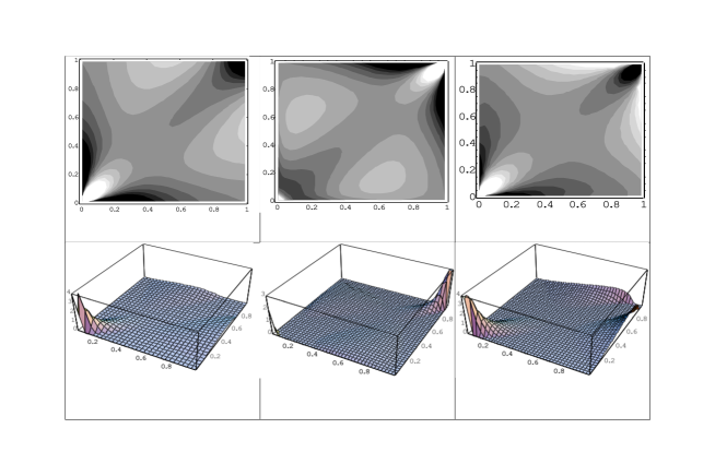
Figure 1: Common comparisons. Copula density differences, through contour plots and 3D plots of synthetic data: Clayton - Frank (left), Gumbel - Frank (center), Clayton - Gumbel (right). Their Kendall’s tau is $0.4$.

Most common scenarios encountered in the literature compare Frank, Clayton, Gumbel, and Gauss copulas with each other, after controlling for some dependence indicator (typically Kendall’s tau): see, for instance, Berg (2009), Genest and Rémillard (2008) and Genest et al. (2009). However, all these pairings produce trivial difference sets $A^{+}$ and $A^{-}$, as revealed in the contour plots and 3D plots of $c_{0}-c_{1}$ of Figure 1. We see that nearly all the mass difference between copula densities $c_{0}$ and $c_{1}$ is concentrated in a single spot, located in either the lower left or upper right corner. Here Kendall’s $\tau=0.4$, but we observed similar plots for different values of $\tau$. Therefore, these common simulation scenarios are tailored towards many standard GOF tests such as KS and CvM tests. We are not aware of any argument that justifies such specific types of pairing, except for analytical tractability. Figures 2 and 3, however, paint a very different scenario with more elaborate difference sets $A^{+}$ and $A^{-}$ that appear in real life situations. How often and to what extent this complex situation is encountered in reality is largely an open empirical issue.

In this study, the copula densities $c_{1}$ were estimated by kernel density estimators based on the following data:

• The bivariate ARCH-like process $(X_{1},Y_{1}),\ldots,(X_{n},Y_{n})$, with $n=10^{6}$, was generated as follows: First, we created independent $Z_{i}\sim N(0,1)$ and $W_{i}=Z_{i}(1+0.6W_{i-1}^{2})^{1/2},$ with $W_{0}=0$. Second, we set $(X_{i},Y_{i}):=(W_{100i},W_{100i+1})$, creating nearly independent couples (of strongly dependent observations). Such models are commonly used in empirical finance, for instance.

• The Mixture Copula data $(X_{1},Y_{1}),\ldots,(X_{n},Y_{n})$, with $n=10^{6}$, are generated from the mixture $c_{1}(s,t)=\frac{1}{2}c_{F}(s,t)+\frac{1}{2}c_{F}(1-s,t)$ for the Frank copula $c_{F}$ with Kendall’s $\tau=0.4$. Therefore, this copula has asymmetrical features, contrary to most copulas that are tested in the literature. Obviously, other asymmetrical copulas could be built, following Liebscher (2008) for instance.

• The Euro-Dollar data $(X_{1},Y_{1}),\ldots,(X_{n},Y_{n})$, with $n=1800,$ are quoted currency exchange values. $X$ is the daily percentage change of the Euro against the US dollar, while $Y$ corresponds to the daily change of the Canadian dollar against the US dollar.

• The Silver-Gold data $(X_{1},Y_{1}),\ldots,(X_{n},Y_{n})$, with $n=5000$, presents the log ratio of the average daily price of silver and gold futures respectively. For instance, $X_{i}=\log(S_{i+1}/S_{i})$ based on the average price $S_{i}$ of silver in US dollars on day $i$.

We compared Mixture copula and ARCH with the independence copula, for which $c_{0}(s,t)=1$ (see Figure 2). In the case of real data (Euro-Dollar and Silver-Gold), we choose the Frank copula density with parameters $\tau=2.6$ and $\tau=3.4$, respectively, for $c_{0}$ (see Figure 3). The latter parameters were chosen after minimizing the (estimated) $L_{1}$-distance between $c_{0}$ and $c_{1}$. The difference sets are easily depicted by dark and bright sections of the contour plots, and the 3D plots clearly indicate that the mass difference between copula densities $c_{0}$ and $c_{1}$ is not concentrated in a single spot.

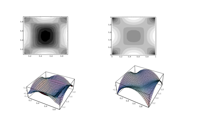
Figure 2: Complex relation (synthetic data). Copula density differences, through contour plots and 3D plots: ARCH (left) and mixture copula (right), compared to the independence copula.

Figure 3: Complex relation (actual data). Copula density differences, through contour plots and 3D plots: Euro - Dollar (left) and Silver - Gold (right), compared to Frank copulas (with Kendall’s tau equal to $2.6$ and $3.4$ respectively).

4.2 GOF tests in practice

We generated the data sets ARCH and Mixture Copula as described above. For each data set, we run two sets of simulations:

• (ARCH-S and Mixture-S) Test the simple null hypothesis $C_{0}(s,t)=st$ using the methodology of Section 2.

• (ARCH-C and Mixture-C) Test the composite null hypothesis that $C_{0}$ is a Frank copula using the procedure described in Section 3.

In both cases, the null hypothesis is wrong and should be rejected.

In our simulations, the number of boxes is $L_{n}=\left\lfloor\ln^{0.95}(n)\right\rfloor-2.$ We approximated the p-values of all the statistics we consider via the bootstrap procedures introduced in sections 2 and 3. For each approximation, we used 1,000 bootstrap samples. For the second set of simulations (ARCH-C and Mixture-C), we computed the parameters $\widehat{\theta}$ and $\widehat{\theta}^{\ast}$ by the usual pseudo-maximum likelihood procedure. Each procedure is repeated 100 times. We report the percentage of times that the computed $p$-value is below $\alpha=0.05$.

Our limited numerical study confirms the above assessment. Table 1 shows that the ATV test outperforms largely the KS and CvM tests in the case of complex pairing, while Table 2 confirms that the ATV test is inferior in case of the commonly used pairings of Figure 1.
In Table 2, for each pair of copulas, say Clayton - Frank, we generated $n$ observations from the first copula (Clayton), and we tested the null hypothesis that the second copula (Frank) is the true underlying copula. In this simple scenario, the sophistication of $\mathbb{T}_{n}$ is a disadvantage compared to simpler usual test statistics. The former test looks for discrepancies everywhere in the unit hypercube (at the price of noise), while the simpler KS and CvM tests pick up easily the right boxes (by chance, in our opinion).
Table 3 shows that the significance level of the ATV test is below $0.05$. The data were simulated from the null hypothesis. In all tables, Kendall’s $\tau=0.4$.

$$\begin{array}[]{cccccc}\text{type}&n&\text{ARCH-S }&\text{ARCH-C}&\text{Mixture-S }&\text{ Mixture-C}\\ \text{ATV}&400&\mathbf{75\%}&\mathbf{80\%}&\mathbf{41\%}&\mathbf{25\%}\\ \text{KS}&400&6\%&4\%&8\%&12\%\\ \text{CvM}&400&25\%&50\%&6\%&15\%\\ \text{ATV}&800&\mathbf{100\%}&\mathbf{99\%}&\mathbf{94\%}&\mathbf{98\%}\\ \text{KS}&800&32\%&50\%&20\%&25\%\\ \text{CvM}&800&50\%&92\%&31\%&84\%\end{array}$$

Table 1: Complex pairing, related to Figure 2: relative frequencies of rejected null hypotheses under $\alpha=0.05$.

$$\begin{array}[]{ccccc}\text{type}&n&\text{Clayton - Frank}&\text{Gumbel - Frank}&\text{ Clayton - Gumbel}\\ \text{ATV}&400&42\%&26\%&88\%\\ \text{KS}&400&58\%&25\%&90\%\\ \text{CvM}&400&\mathbf{84\%}&\mathbf{47\%}&\mathbf{95\%}\\ \text{ATV}&800&92\%&58\%&94\%\\ \text{KS}&800&98\%&53\%&98\%\\ \text{CvM}&800&\mathbf{100\%}&\mathbf{73\%}&\mathbf{100\%}\end{array}$$

Table 2: Trivial pairing, related to Figure 1: relative frequencies of rejected null hypotheses under $\alpha=0.05.$

$$\begin{array}[]{ccccc}\text{type}&n&\text{Clayton - Clayton}&\text{Gumbel - Gumbel}&\text{ Frank -Frank}\\ \text{ATV}&400&3\%&2\%&2\%\\ \text{KS}&400&4\%&5\%&4\%\\ \text{CvM}&400&4\mathbf{\%}&5\mathbf{\%}&4\mathbf{\%}\\ \text{ATV}&800&2\%&4\%&3\%\\ \text{KS}&800&3\%&3\%&5\%\\ \text{CvM}&800&5\mathbf{\%}&3\mathbf{\%}&6\mathbf{\%}\end{array}$$

Table 3: Errors of the first kind: relative frequencies of rejected null hypotheses under $\alpha=0.05$.

5 Proofs

Throughout the proofs, we assume without loss of generality that $F_{j}=I$ for every $j=1,\ldots,d$ (uniform marginal distributions). This implies that $H=C$. This is justified by the following lemma.

Lemma 8.

Let $F_{j}$, $j=1,\ldots,d$ be continuous distribution functions. Denote by $\tilde{H}$ the cdf of $(F_{1}(X_{1}),\ldots,F_{d}(X_{d}))$ and by $\tilde{C}$ its associated copula. The empirical copula associated to the sample $(F_{1}(X_{i1}),\ldots,F_{d}(X_{id}))$, ${i=1,\ldots,n}$, is denoted by $\tilde{\mathbb{C}}_{n}$. We have

$$C(\mathbf{u})=\tilde{C}(\mathbf{u})=\tilde{H}(\mathbf{u})\text{ for all }\mathbf{u}\in[0,1]^{d}.$$

Moreover,

$${\mathbb{C}}_{n}\left(\frac{i_{1}}{n},\ldots,\frac{i_{d}}{n}\right)=\tilde{\mathbb{C}}_{n}\left(\frac{i_{1}}{n},\ldots,\frac{i_{d}}{n}\right)\text{ for }i_{1},\ldots,i_{d}\in\{0,1,\ldots,n\}.$$

Proof.

This is a straightforward extension of Lemma 1 in Fermanian et al. (2004). ∎

Since the letter $C$ is reserved for the copula function, we use the letters $K,K_{0},K_{1}$, etc. in the sequel to denote generic constants, and we write $\|\mathbf{s}\|_{\infty}=\max_{1\leq j\leq d}|s_{j}|$ of $\mathbf{s}=(s_{1},\ldots,s_{d})\in[0,1]^{d}$.

5.1 Proof of preliminary results

In general, note that, for each $f\in\mbox{$\mathcal{F}$}_{n}$ defined in (2.1), we can write

$$\mathbb{Z}_{n}(f)=\sum_{k=1}^{L_{n}}c_{k}\mathbb{Z}_{n}(B_{k})=\sum_{l=1}^{2^{d}L_{n}}\sigma_{l}\mathbb{Z}_{n}(\mathbf{s}_{l}),$$

and

$$\mathbb{Z}_{n}^{*}(f)=\sum_{l=1}^{2^{d}L_{n}}\sigma_{l}\mathbb{Z}_{n}^{*}(\mathbf{s}_{l}),$$

for some $\sigma_{l}\in\{-1,+1\}$ and $\mathbf{s}_{l}\in[0,1]^{d}$, using formula (1.5). Let $\alpha_{n}(\mathbf{u}):=\sqrt{n}(\mathbb{H}_{n}-H)(\mathbf{u})=\sqrt{n}(\mathbb{H}_{n}(\mathbf{u})-\mathbf{u})$ be the ordinary uniform empirical process in $[0,1]^{d}$, and let its oscillation modulus be defined as

$$\mathbb{M}_{n}(\delta):=\sup\left\{\left|\alpha_{n}(\mathbf{s})-\alpha_{n}(\mathbf{s}^{\prime})\right|:\ \|\mathbf{s}-\mathbf{s}^{\prime}\|_{\infty}\leq\delta;\,\mathbf{s},\mathbf{s}^{\prime}\in[0,1]^{d}\right\},$$ (5.1)

for any $\delta>0$.

Lemma 9.

Let $(\delta_{n})_{n\geq 0}$ be a sequence of positive real numbers such that $n\delta_{n}/\log n\rightarrow\infty$. Then, we have

$$\mathbb{M}_{n}(\delta_{n})=O(\delta_{n}^{1/2}(\log n)^{1/2})\qquad\text{almost surely}.$$

Proof.

We apply Proposition 14 with $\lambda_{n}=K_{0}\delta^{1/2}_{n}(\log n)^{1/2}$ for some constant $K_{0}>0$. Since $n^{-1/2}\lambda_{n}/\delta_{n}=K_{0}\left(\log n/(n\delta_{n})\right)^{1/2}$ tends to zero, this inequality can be rewritten

$$\mathbb{P}\left\{\mathbb{M}_{n}(\delta_{n})>\lambda_{n}\right\}\leq\frac{K_{1}}{\delta_{n}}\exp\left(-\frac{K_{2}\psi(1)\lambda^{2}_{n}}{\delta_{n}}\right)=K_{1}n\exp\left(-K_{2}K_{0}^{2}\psi(1)\log n\right),$$

for some constants $K_{1}$, $K_{2}$ and $n$ sufficiently large. When $K_{0}$ is sufficiently large, we check that

$$\mathbb{P}\left\{\mathbb{M}_{n}(\delta_{n})>\lambda_{n}\right\}\leq\frac{K_{3}}{n^{2}},$$

for some constant $K_{3}$. Invoke the Borel-Cantelli Lemma to conclude the proof. ∎

In addition, let $\alpha_{n,j}(u)=\sqrt{n}(\mathbb{F}_{n,j}-F_{j})(u)=\sqrt{n}(\mathbb{F}_{n,j}(u)-u)$ be the ordinary uniform (marginal) empirical process in $[0,1]$, and we define

$$\widetilde{\mathbb{Z}}_{n}(\mathbf{s})=\alpha_{n}(\mathbf{s})-\sum_{j=1}^{d}C_{j}(\mathbf{s})\alpha_{n,j}(s_{j}).$$ (5.2)

Proposition 10.

Under conditions (C1) and (C2), we have

$$\lim_{n\rightarrow\infty}\sup_{h\in BL_{1}}\left|\mathbb{E}[h(\mathbb{Z}_{n})]-\mathbb{E}[h(\widetilde{\mathbb{Z}}_{n})]\right|=0.$$

Proof.

First, we observe that

$$\sup_{h\in BL_{1}}\left|\mathbb{E}[h(\mathbb{Z}_{n})-h(\widetilde{\mathbb{Z}}_{n})]\right| \leq \delta+2\mathbb{P}\left\{\sup_{f\in\mbox{$\mathcal{F}$}_{n}}|\mathbb{Z}_{n}(f)-\widetilde{\mathbb{Z}}_{n}(f)|>\delta\right\}.$$

The latter inequality holds for any $\delta>0$, and uses the fact that $|h|$ is bounded by 1 and has Lipschitz constant 1. It remains to show that

$$\sup_{f\in\mbox{$\mathcal{F}$}_{n}}|\mathbb{Z}_{n}(f)-\widetilde{\mathbb{Z}}_{n}(f)|\rightarrow 0,$$

in probability, as $n\rightarrow\infty$. The remainder of the proof generalizes Proposition 4.2 of Segers (2012). Now, we note that

$$\sup_{f\in\mbox{$\mathcal{F}$}_{n}}|\mathbb{Z}_{n}(f)-\widetilde{\mathbb{Z}}_{n}(f)|\leq 2^{d}L_{n}\sup_{\mathbf{s}\in[0,1]^{d}}|\mathbb{Z}_{n}(\mathbf{s})-\widetilde{\mathbb{Z}}_{n}(\mathbf{s})|\leq 2^{d}L_{n}(I+II)$$

with

$$I = \sup_{\mathbf{s}\in[0,1]^{d}}\left|\alpha_{n}(\mathbb{F}_{n,1}^{-}s_{1},\ldots,\mathbb{F}_{n,d}^{-}s_{d})-\alpha_{n}(\mathbf{s})\right|,$$

$$II = \sup_{\mathbf{s}\in[0,1]^{d}}\left|\sqrt{n}\left[C(\mathbb{F}_{n,1}^{-}s_{1},\ldots,\mathbb{F}_{n,d}^{-}s_{d})-C(\mathbf{s})\right]+\sum_{j=1}^{d}C_{j}(\mathbf{s})\alpha_{n,j}(s_{j})\right|.$$

The first term, $I$, can be bounded as follows. Set $\beta_{n,j}(s)=\sqrt{n}(\mathbb{F}_{n,j}^{-}s-s)$, $j=1,\ldots,d$. By the Chung-Smirnov LIL, we have

$$\max_{1\leq j\leq d}\sup_{0\leq s\leq 1}|\beta_{n,j}(s)|=O((\log\log n)^{1/2})\qquad\text{ almost surely}.$$

Using Lemma 9 with $\delta=n^{-1/2}(\log\log n)^{1/2}$, we get

$$\sup_{\|\mathbf{s}-\mathbf{s}^{\prime}\|_{\infty}<\delta}\left|\alpha_{n}(\mathbf{s})-\alpha_{n}(\mathbf{s}^{\prime})\right|=O(n^{-1/4}(\log n)^{1/2}(\log\log n)^{1/4}),$$

almost surely. This implies that $I=O(n^{-1/4}(\log n)^{1/2}(\log\log n)^{1/4})$, almost surely.

For the second term, we get by the mean value theorem that

$$II = \sup_{\mathbf{s}\in[0,1]^{d}}\left|\sqrt{n}[C(\mathbb{F}_{n,1}^{-}s_{1},\ldots,\mathbb{F}_{n,d}^{-}s_{d})-C(\mathbf{s})]+\sum_{j=1}^{d}C_{j}(\mathbf{s})\alpha_{n,j}(s_{j})\right|$$

$$\leq \sup_{\mathbf{s}\in[0,1]^{d}}\left|\sum_{j=1}^{d}C_{j}(\mathbf{s}_{n})\beta_{nj}(s_{j})+\sum_{j=1}^{d}C_{j}(\mathbf{s})\alpha_{n,j}(s_{j})\right|,$$

where $\mathbf{s}_{n}$ is a vector in $[0,1]^{d}$ s.t. $\|\mathbf{s}_{n}-\mathbf{s}\|_{\infty}\leq n^{-1/2}\max_{1\leq j\leq d}|\beta_{n,j}(s_{j})|$. Since $|C_{j}|\leq 1$ for every $j=1,\ldots,d$ (because copulas are Lipschitz with Lipschitz constant 1), we deduce

$$II \leq \sup_{\mathbf{s}\in[0,1]^{d}}\sum_{j=1}^{d}\left|\beta_{nj}(s_{j})+\alpha_{n,j}(s_{j})\right|+\sup_{\mathbf{s}\in[0,1]^{d}}\sum_{j=1}^{d}\left|[C_{j}(\mathbf{s}_{n})-C_{j}(\mathbf{s})]\alpha_{n,j}(s_{j})\right|$$

$$\leq IIa+IIb.$$

The Bahadur-Kiefer theorem (Shorack and Wellner, 2009, p. 585) states that

$$\max_{1\leq j\leq d}\sup_{0\leq s\leq 1}|\beta_{n,j}(s)+\alpha_{n,j}(s_{j})|=O(n^{-1/4}(\log n)^{1/2}(\log\log n)^{1/4})\quad\text{almost surely}.$$

Then, $IIa=O(n^{-1/4}(\log n)^{1/2}(\log\log n)^{1/4})$ almost surely.

Concerning $IIb$, we consider a positive sequence $(\varepsilon_{n})$, $\varepsilon_{n}\rightarrow 0$, that will be specified later independently of any $\mathbf{s}=(s_{1},\ldots,s_{d})\in[0,1]^{d}$. For any index $j=1,\ldots,d$ and any $\mathbf{s}\in[0,1]^{d}$, we will distinguish the two cases: $s_{j}\in[\varepsilon_{n},1-\varepsilon_{n}]$ and the opposite.

If $s_{j}\in[\varepsilon_{n},1-\varepsilon_{n}]$ then

$$s_{nj}=s_{j}\left(1+\frac{s_{nj}-s_{j}}{s_{j}}\right)\geq s_{j}\left(1-\frac{|s_{nj}-s_{j}|}{\varepsilon_{n}}\right)\geq\frac{s_{j}}{2},$$

and

$$1-s_{nj}\geq(1-s_{j})\left(1-\frac{|s_{nj}-s_{j}|}{\varepsilon_{n}}\right)\geq\frac{1-s_{j}}{2},$$

almost surely and for $n$ sufficiently large, for all $\varepsilon_{n}\rightarrow 0$ and $n\varepsilon_{n}^{2}/\log n\rightarrow\infty$. Corollary 2 in Mason (1981) implies that

$$\max_{1\leq j\leq d}\sup_{0\leq s_{j}\leq 1}|s_{j}^{-1/2}(1-s_{j})^{-1/2}\alpha_{n,j}(s_{j})|\leq K(\log n)^{1/2}\log\log n,$$

almost surely, for some constant $K>0$.

In this case, using condition (C1), we deduce,

$$\left|C_{j}(\mathbf{s}_{n})-C_{j}(\mathbf{s})\right||\alpha_{n,j}(s_{j})| \leq K_{0}\|\mathbf{s}_{n}-\mathbf{s}\|^{r}\left\{s_{j}^{-\beta}(1-s_{j})^{-\beta}+s_{nj}^{-\beta}(1-s_{nj})^{-\beta}\right\}|\alpha_{n,j}(s_{j})|$$

$$\leq K_{1}\|\mathbf{s}_{n}-\mathbf{s}\|^{r}s_{j}^{1/2-\beta}(1-s_{j})^{1/2-\beta}(\log n)^{1/2}\log\log n$$

$$\leq K_{2}n^{-r/2}(\log\log n)^{r/2}\max(\varepsilon_{n}^{1/2-\beta},1)(\log n)^{1/2}\log\log n,$$

almost surely, for some constants $K_{0},K_{1},K_{2}>0$ and every $j$.

If $s_{j}\not\in[\varepsilon_{n},1-\varepsilon_{n}]$ then

$$\left|C_{j}(\mathbf{s}_{n})-C_{j}(\mathbf{s})\right||\alpha_{n,j}(s_{j})| \leq 2|\alpha_{n,j}(s_{j})|$$

$$\leq 2\varepsilon_{n}^{1/2}s_{j}^{-1/2}(1-s_{j})^{-1/2}|\alpha_{n,j}(s_{j})|$$

$$\leq K\varepsilon_{n}^{1/2}(\log n)^{1/2}\log\log n\ \text{ almost surely,}$$

see Corollary 2 in Mason (1981).

Combining all these bounds entails then

$$IIb\leq K_{3}\left[n^{-r/2}(\log\log n)^{r/2}\max(\varepsilon_{n}^{1/2-\beta},1)+\varepsilon_{n}^{1/2}\right](\log n)^{1/2}\log\log n,$$

with $K_{3}>0$. We now specify the choice of $\varepsilon_{n}=n^{-p}$, with $p$ depending on $\beta$ and $r$ only. If $2\beta>2r+1$, we take $0<p<r/(2\beta-1)$. If $\beta<1/2$, set $p=1/4$. Otherwise, take $p=\min(1/4,r/(4\beta-2))$, for instance. In each case, these choices ensure that $IIb=O(n^{-q})$ almost surely, for some $q>0$.

Since $L_{n}=O(\log n)$ by assumption (C2), we obtain $L_{n}(I+II)\rightarrow 0$ almost surely, as $n\rightarrow\infty$, and the proof is complete. ∎

Next, we turn our attention to the bootstrap counterparts. We define $\alpha_{n}^{*}(\mathbf{s})=\sqrt{n}(\mathbb{H}_{n}^{*}-\mathbb{H}_{n})(\mathbf{s})$ as the ordinary bootstrap empirical process in $[0,1]^{d}$. We prove the following exponential inequality for the oscillation modulus

$$\mathbb{M}_{n}^{*}(\delta)=\sup_{\|\mathbf{s}-\mathbf{s}^{\prime}\|_{\infty}<\delta}|\alpha_{n}^{*}(\mathbf{s})-\alpha_{n}^{*}(\mathbf{s}^{\prime})|.$$

Lemma 11.

For all bounded sequences $\delta_{n}$ such that $n\delta_{n}/\log(n)\rightarrow\infty$ as $n\rightarrow\infty$,

$$\mathbb{M}_{n}^{*}(\delta_{n})=O(\delta_{n}^{1/2}(\log n)^{1/2})\ \quad\text{almost surely.}$$ (5.3)

Note that the sequence $(\delta_{n})$ may be constant.

Proof.

Since $\alpha_{n}^{*}$ is a step function, we find that

$$\sup_{\ \|\mathbf{s}-\mathbf{s}^{\prime}\|_{\infty}<\delta_{n}}|\alpha_{n}^{*}(\mathbf{s})-\alpha_{n}^{*}(\mathbf{s}^{\prime})|=\max|\alpha_{n}^{*}(X_{i_{1},1},\ldots,X_{i_{d},d})-\alpha_{n}^{*}(X_{i^{\prime}_{1},1},\ldots,X_{i^{\prime}_{d},d})|,$$

with the maximum taken over all $|X_{i_{j},j}-X_{i^{\prime}_{j},j}|<\delta_{n}$, $j=1,\ldots,d$, $i_{1},i^{\prime}_{1},\ldots,i_{d},i^{\prime}_{d}\in\{1,\ldots,n\}$. For any $\mathbf{i}:=(i_{1},\ldots,i_{d})$ and $\mathbf{i}^{\prime}=(i_{1}^{\prime},\ldots,i_{d}^{\prime})$ in $\{1,\ldots,n\}^{d}$, we rewrite

$$|\alpha_{n}^{*}(X_{i_{1},1},\ldots,X_{i_{d},d})-\alpha_{n}^{*}(X_{i^{\prime}_{1},1},\ldots,X_{i^{\prime}_{d},d})|=n^{-1/2}\sum_{k=1}^{n}\{V_{k,\mathbf{i},\mathbf{i}^{\prime}}-\mathbb{E}^{*}[V_{k,\mathbf{i},\mathbf{i}^{\prime}}]\},$$

as a sum of bounded independent random variables with

$$V_{k,\mathbf{i},\mathbf{i}^{\prime}}:=\mathbf{1}\{X_{k,j}^{*}\leq X_{i_{j},j},\,j=1,\ldots,d\}-\mathbf{1}\{X_{k,j}^{*}\leq X_{i^{\prime}_{j},j},\,j=1,\ldots,d\},$$

conditionally on the sample $(\mathbf{X}_{1},\ldots,\mathbf{X}_{n})$. Moreover, a simple calculation and Lemma 9 yield

$$\text{Var}^{*}(V_{k,\mathbf{i},\mathbf{i}^{\prime}}) \leq \sum_{j=1}^{d}\mathbb{P}^{*}\left\{\min(X_{i_{j},j},X_{i_{j}^{\prime},j})\leq X_{k,j}^{*}\leq\max(X_{i_{j},j},X_{i_{j}^{\prime},j})\right\}$$

$$\leq \sum_{j=1}^{d}\sup_{s_{j}}[\mathbb{F}_{n,j}(s_{j}+\delta_{n})-\mathbb{F}_{n,j}(s_{j})]$$

$$\leq d\delta_{n}+dn^{-1/2}\mathbb{M}_{n}(\delta_{n})$$

$$\leq d\max(\delta_{n},\mathbb{M}_{n}(\delta_{n})/\sqrt{n})$$

$$\leq K\max(\delta_{n},\sqrt{\delta_{n}\log n}/\sqrt{n})=K\delta_{n},$$

for $n$ large enough, for almost all realizations and for some constant $K>0$. Hence, by the union bound and Bernstein’s exponential inequality for bounded random variables, we have, for some constant $K_{0}$,

$$\mathbb{P}^{*}\left\{\max_{\begin{subarray}{c}\mathbf{i},\mathbf{i}^{\prime}\in\{1,\ldots,n\}^{d}\\ |X_{i_{j},j}-X_{i^{\prime}_{j},j}|<\delta_{n},\;\forall j\end{subarray}}|\alpha_{n}^{*}(X_{i_{1},1},\ldots,X_{i_{d},d})-\alpha_{n}^{*}(X_{i^{\prime}_{1},1},\ldots,X_{i^{\prime}_{d},d})|>x\right\}$$

$$\leq 2n^{2d}\exp\left(-K_{0}(\sqrt{n}x\wedge x^{2}\delta_{n}^{-1})\right),$$

for all samples $(\mathbf{X}_{1},\ldots,\mathbf{X}_{n})$. By integrating the previous inequality over $\mathbb{P}$, we get the same inequality, but replacing $\mathbb{P}^{*}$ by $\mathbb{P}$. Set $x=K_{1}\delta_{n}^{1/2}(\log n)^{1/2}$ and take a constant $K_{1}$ sufficiently large to obtain

$$\sum_{n=1}^{+\infty}\mathbb{P}\left\{\mathbb{M}_{n}^{*}(\delta_{n})>K_{1}\delta_{n}^{1/2}(\log n)^{1/2}\right\}<+\infty.$$

Apply the Borel-Cantelli lemma to conclude the proof. ∎

Analogous to the approximation of the process $\mathbb{Z}_{n}$ by $\widetilde{\mathbb{Z}}_{n}$ before, we introduce a simpler process $\widetilde{\mathbb{Z}}_{n}^{*}$ to approximate $\mathbb{Z}_{n}^{*}$. Set

$$\widetilde{\mathbb{Z}}_{n}^{*}(\mathbf{s})=\sqrt{n}(\mathbb{H}_{n}^{*}-\mathbb{H}_{n})(\mathbf{s})-\sum_{j=1}^{d}C_{j}(\mathbf{s})\sqrt{n}(\mathbb{F}_{n,j}^{*}-\mathbb{F}_{n,j})(s_{j}).$$ (5.4)

Proposition 12.

Under conditions (C1) and (C2), we have

$$\lim_{n\rightarrow\infty}\mathbb{E}\left[\sup_{h\in BL_{1}}\left|\mathbb{E}^{*}[h(\mathbb{Z}_{n}^{*})-h(\widetilde{\mathbb{Z}}_{n}^{*})]\right|\right]=0.$$

Proof.

First, we notice that, for any $\eta>0$,

$$\mathbb{E}\left[\sup_{h\in BL_{1}}\left|\mathbb{E}^{*}[h(\mathbb{Z}_{n}^{*})-h(\widetilde{\mathbb{Z}}_{n}^{*})]\right|\right] \leq \eta+2\mathbb{E}\left[\mathbb{P}^{*}\left\{\sup_{f\in\mbox{$\mathcal{F}$}_{n}}\left|\mathbb{Z}_{n}^{*}(f)-\widetilde{\mathbb{Z}}_{n}^{*}(f)\right|\geq\eta\right\}\right]$$

$$\leq \eta+2\mathbb{E}\left[\mathbb{P}^{*}\left\{\sup_{{\bf s}}2^{d}L_{n}\left|\mathbb{Z}_{n}^{*}({\bf s})-\widetilde{\mathbb{Z}}_{n}^{*}({\bf s})\right|\geq\eta\right\}\right].$$

Some straightforward adding and subtracting yields $\mathbb{Z}_{n}^{*}(\mathbf{s})=\bar{\mathbb{Z}}_{n}^{*}(\mathbf{s})+R_{n}^{*}(\mathbf{s})$ with

$$\bar{\mathbb{Z}}_{n}^{*}(\mathbf{s})=\sqrt{n}\{\mathbb{H}^{*}_{n}(\mathbf{s})-\mathbb{H}_{n}(\mathbf{s})\}-\sqrt{n}\{C(\mathbb{F}_{n,1}^{*}s_{1},\ldots,\mathbb{F}_{n,d}^{*}s_{d})-C(\mathbb{F}_{n,1}s_{1},\ldots,\mathbb{F}_{n,d}s_{d})\}$$

and $R_{n}^{*}(\mathbf{s})=R_{n,1}^{*}(\mathbf{s})+R_{n,2}^{*}(\mathbf{s})+R_{n,3}^{*}(\mathbf{s})+R_{n,4}^{*}(\mathbf{s})$ with

$$R_{n,1}^{*}(\mathbf{s}) = \alpha_{n}^{*}(\mathbb{F}_{n,1}^{*-}s_{1},\ldots,\mathbb{F}_{n,d}^{*-}s_{d})-\alpha_{n}^{*}(\mathbb{F}_{n,1}^{-}s_{1},\ldots,\mathbb{F}_{n,d}^{-}s_{d})$$

$$R_{n,2}^{*}(\mathbf{s}) = \alpha_{n}^{*}(\mathbb{F}_{n,1}^{-}s_{1},\ldots,\mathbb{F}_{n,d}^{-}s_{d})-\alpha_{n}^{*}(\mathbf{s})$$

$$R_{n,3}^{*}(\mathbf{s}) = \alpha_{n}(\mathbb{F}_{n,1}^{*-}s_{1},\ldots,\mathbb{F}_{n,d}^{*-}s_{d})-\alpha_{n}(\mathbb{F}_{n,1}^{-}s_{1},\ldots,\mathbb{F}_{n,d}^{-}s_{d})$$

$$R_{n,4}^{*}(\mathbf{s}) = \sqrt{n}\left\{C(\mathbb{F}_{n,1}^{*-}s_{1},\ldots,\mathbb{F}_{n,d}^{*-}s_{d})-C(\mathbb{F}_{n,1}^{-}s_{1},\ldots,\mathbb{F}_{n,d}^{-}s_{d})\right\}$$

$$+\sqrt{n}\left\{C(\mathbb{F}_{n,1}^{*}s_{1},\ldots,\mathbb{F}_{n,d}^{*}s_{d})-C(\mathbb{F}_{n,1}s_{1},\ldots,\mathbb{F}_{n,d}s_{d})\right\}.$$

Let $\alpha_{n,j}^{*}(s)=\sqrt{n}(\mathbb{F}_{n,j}^{*}-\mathbb{F}_{n,j})(s)$ and $\beta_{n,j}^{*}(s)=\sqrt{n}(\mathbb{F}_{n,j}^{-*}-\mathbb{F}_{n,j}^{-})(s)$ be the bootstrap versions of the empirical processes $\alpha_{n,j}(s)$ and $\beta_{n,j}(s)$, respectively. Both converge to the same weak limit as

$$\sup_{0\leq s_{j}\leq 1}|\beta_{n,j}^{*}(s_{j})+\alpha_{n,j}^{*}(s_{j})|=O(n^{-1/4}(\log n)^{1/2}(\log\log n)^{1/4})\quad\text{ almost surely},$$

see displays (2.10’) and (2.12’) in Theorem 2.1 of Csörgó and Mason (1989). It remains to show that $\mathbb{P}^{*}\{L_{n}\sup_{\mathbf{s}}|R_{n}^{*}(\mathbf{s})|>\eta\}\rightarrow 0$ for all $\eta>0$, conditionally given all sequences $(\mathbf{X}_{1},\ldots,\mathbf{X}_{n})\in\Omega_{n}$ for some sequence of events $\Omega_{n}\subset\mathbb{R}^{d\times n}$ with $\lim_{n\rightarrow\infty}\mathbb{P}(\Omega_{n})=1$.

Let $\delta_{n}=n^{-1/4}$. (Other choices are possible as well.) We have

$$\limsup_{n\rightarrow\infty}\mathbb{P}^{*}\{L_{n}\|R_{n,1}^{*}\|_{\infty}\geq\eta\}\leq\limsup_{n\rightarrow\infty}\mathbb{P}^{*}\{L_{n}\mathbb{M}_{n}^{*}(\delta_{n})\geq\eta\}+\limsup_{n\rightarrow\infty}\mathbb{P}^{*}\{\max_{j}\|\beta_{n,j}^{*}\|_{\infty}\geq\sqrt{n}\delta_{n}\}=0,$$

by Lemma 11. Next, on the event $\max_{j}\|\beta_{n,j}\|_{\infty}\leq\sqrt{n}\delta_{n}$ (that holds almost surely by the law of iterated logarithm),

$$\limsup_{n\rightarrow\infty}\mathbb{P}^{*}\{L_{n}\|R_{n,2}^{*}\|_{\infty}\geq\eta\}\leq\limsup_{n\rightarrow\infty}\mathbb{P}^{*}\{L_{n}\mathbb{M}_{n}^{*}(\delta_{n})\geq\eta\}=0,$$

by Lemma 11. On the event $L_{n}\mathbb{M}_{n}(\delta_{n})<\eta$ (that holds almost surely by Lemma 9), we have

$$\limsup_{n\rightarrow\infty}\mathbb{P}^{*}\{L_{n}\|R^{*}_{n,3}\|_{\infty}\geq\eta\}\leq\limsup_{n\rightarrow\infty}\mathbb{P}^{*}\{\max_{j}\|\beta_{n,j}^{*}\|_{\infty}>\sqrt{n}\delta_{n}\}=0$$

by the weak convergence of $\beta_{n,j}^{*}$. Finally, for some $s_{j}^{*}$ between $\mathbb{F}_{n,j}^{-*}(s_{j})$ and $\mathbb{F}_{n,j}^{-}(s_{j})$, and $s_{j}^{**}$ between $\mathbb{F}_{n,j}^{*}(s_{j})$ and $\mathbb{F}_{n,j}(s_{j})$, we have

$$|R^{*}_{n,4}(\mathbf{s})| = \left|\sum_{j=1}^{d}\{C_{j}(s_{j}^{*})\beta_{n,j}^{*}(s_{j})+C_{j}(s_{j}^{**})\alpha_{n,j}^{*}(s_{j})\right|$$

$$\leq \sum_{j=1}^{d}|\beta_{n,j}^{*}(s_{j})+\alpha_{n,j}^{*}(s_{j})|+\sum_{j=1}^{d}|\alpha_{n,j}^{*}(s_{j})||C_{j}(s_{j}^{*})-C_{j}(s_{j}^{**})|.$$

The first term is of order $O(n^{-1/4}(\log n)^{1/2}(\log\log n)^{1/4})$, uniformly in $s_{j}$. For the second term, we argue as in the proof of Proposition 10. First, we observe that $|s_{j}^{**}-s_{j}^{*}|\leq|s_{j}^{*}-s_{j}|+|s_{j}^{**}-s_{j}|$ is of order $O_{p^{*}}(n^{-1/2})$. Second, since the class $\mathbf{1}\{x\leq t\}t^{-b}(1-t)^{-b}$ is a $P$-Donsker class for the uniform probability measure $P$ on $[0,1]$, for all $0\leq b<1/2$, see Van der Vaart and Wellner (1996), Example 2.11.15 (page 214), the weak convergence of the bootstrap empirical process [Van der Vaart and Wellner (1996, Theorem 3.6.1, page 347)] implies that

$$\sup_{0<s<1}|\alpha_{n,j}^{*}(s)|/(s^{b}(1-s)^{b})=O_{p^{*}}(1).$$

Consequently, as in the proof of Proposition 10, we find that, for some constant $K<\infty$,

$$\sup_{\varepsilon_{n}\leq s_{j}\leq 1-\varepsilon_{n}}|\alpha_{n,j}^{*}(s_{j})||C_{j}(s_{j}^{*})-C_{j}(s_{j}^{**})| \leq K|s_{j}^{**}-s_{j}^{*}|^{r}s_{j}^{b-\beta}(1-s_{j})^{b-\beta}\sup_{s_{j}}|\alpha_{n,j}^{*}(s_{j})|/(s^{b}(1-s)^{b})$$

which is of order $O_{p^{*}}(1)\cdot\max(n^{-r/2}\max(1,\varepsilon_{n}^{b-\beta})$. On the other side,

$$\sup_{s_{j}\not\in[\varepsilon,1-\varepsilon_{n}]}|\alpha_{n,j}^{*}(s_{j})||C_{j}(s_{j}^{*})-C_{j}(s_{j}^{**})| \leq 2\sup_{s_{j}\not\in[\varepsilon,1-\varepsilon_{n}]}|\alpha_{n,j}^{*}(s_{j})|$$

$$\leq 2\varepsilon_{n}^{b}\sup_{s_{j}}|\alpha_{n,j}^{*}(s_{j})|/(s^{b}(1-s)^{b}),$$

which is of order $O_{p^{*}}(\varepsilon_{n}^{b})$. Combining both bounds yields $\sup_{\mathbf{s}}|R_{n,4}(\mathbf{s})|=O_{p^{*}}(\varepsilon_{n}^{b}+n^{-r/2}\max(1,\varepsilon_{n}^{b-\beta}))$. Taking $\varepsilon_{n}=n^{-p}$ with $p$ depending on $b,\beta$ and $r$, we get that $\lim_{n\rightarrow\infty}\mathbb{P}^{*}\{L_{n}\sup_{\mathbf{s}}|R^{*}_{n,4}(\mathbf{s})|\geq\eta\}=0$ for all $\eta>0$, conditionally on all sequences $(\mathbf{X}_{1},\ldots,\mathbf{X}_{n})\in\Omega_{n}$ for some sequence of events $\Omega_{n}$ with $\lim_{n}\mathbb{P}(\Omega_{n})=1$. This completes our proof. ∎

5.2 Proof of Theorem 1

By triangle inequality, we have,

$$\mathbb{E}\left[\sup_{h\in BL_{1}}\left|h(\mathbb{Z}_{n})]-\mathbb{E}^{*}[h(\mathbb{Z}_{n}^{\ast})]\right|\right] \leq \sup_{h\in BL_{1}}\left|\mathbb{E}[h(\mathbb{Z}_{n})-h(\widetilde{\mathbb{Z}}_{n})]\right|$$

$$+\mathbb{E}\left[\sup_{h\in BL_{1}}\left|\mathbb{E}[h(\widetilde{\mathbb{Z}}_{n})]-\mathbb{E}^{*}[h(\widetilde{\mathbb{Z}}_{n}^{*})]\right|\right]$$

$$+\mathbb{E}\left[\sup_{h\in BL_{1}}\left|\mathbb{E}^{*}[h(\widetilde{\mathbb{Z}}_{n}^{*})-h(\mathbb{Z}_{n}^{*})]\right|\right].$$

In view of Proposition 10 and Proposition 12, it remains to show that the second term on the right is asymptotically negligible. We recall that

$$\widetilde{\mathbb{Z}}_{n}(f) = \sum_{k=1}^{2^{d}L_{n}}\sigma_{k}\widetilde{\mathbb{Z}}_{n}(\mathbf{s}_{k})=\sum_{k=1}^{2^{d}L_{n}}\sigma_{k}\int f_{k}(\mathbf{x})\,d\alpha_{n}(\mathbf{x}),$$

for

$$f_{k}(\mathbf{x})=\mathbf{1}\{\mathbf{x}\leq\mathbf{s}_{k}\}-\sum_{j=1}^{d}C_{j}(\mathbf{s}_{k})\mathbf{1}\{x_{j}\leq s_{k,j}\}.$$

Now, let $h_{f}(\mathbf{x})=\sum_{k=1}^{2^{d}L_{n}}\sigma_{k}f_{k}(\mathbf{x})$ so that

$$\widetilde{\mathbb{Z}}_{n}(f)=\int h_{f}\,d\alpha_{n},$$ (5.5)

and we can derive in the same way

$$\widetilde{\mathbb{Z}}_{n}^{*}(f)=\int h_{f}\,d\alpha_{n}^{*}.$$ (5.6)

We now apply Theorem 3 in Radulović (2012), stated as Theorem 13 in the appendix for convenience. We need to verify that

• the $d+1$ classes

  $$\mbox{$\mathcal{G}$}_{k}^{a} = \left\{\mathbf{1}\{\mathbf{x}\leq\mathbf{s}_{k}\},\ \mathbf{s}_{k}\in[0,1]^{d}\right\},$$

  $$\mbox{$\mathcal{G}$}_{k}^{(j)} = \left\{C_{j}(\mathbf{s}_{k})\mathbf{1}\{x\leq s_{k,j}\},\ \mathbf{s}_{k}\in[0,1]^{d}\right\},\;j=1,\ldots,d,$$

  have VC–indices $V_{k}^{a}$ and $V_{k}^{(j)}$, respectively, with $\sum_{k=1}^{2^{d}L_{n}}(V_{k}^{a}+\sum_{j=1}^{d}V_{k}^{(j)})\leq K(\log n)^{\gamma}$ for some finite constant $K$ and some $0<\gamma<1$.

• the class $\mathcal{H}_{n}=\{h_{f}$ : $\ f\in\mathcal{F}_{n}\}$ has an envelope $H(\mathbf{x})$ with $\mathbb{E}[H^{4}(\mathbf{X})]<\infty$.

First we verify the VC property. The class $\mathcal{G}_{k}^{a}$ is VC with VC-dimension $V_{k}^{a}=d+1$ (Van der Vaart and Wellner, 2000, page 135), while the class $\mbox{$\mathcal{G}$}_{k}^{(j)}$ is a subclass of the class of functions $c\mathbf{1}\{a\leq x\leq b\}$ with $a,b\in\mathbb{R}$ and $c>0$. This class has a VC index $3$ : see van der Vaart and Wellner (2000), Problem 20, page 153. Consequently

$$\sum_{k=1}^{2^{d}L_{n}}(V_{k}^{a}+\sum_{j=1}^{d}V_{k}^{(j)})\leq(4d+1)2^{d}L_{n}\leq K(\log n)^{\gamma}$$

for some $K<\infty$.

It remains to verify the envelope condition. We will show that $h_{f}(\textbf{x})$ has envelope $1+d+\sum_{j=1}^{d}TV(C_{j})$. Writing

$$g_{\mathbf{x}}(\mathbf{s}) = \mathbf{1}\{\mathbf{x}\leq\mathbf{s}\}-\sum_{j=1}^{d}C_{j}(\mathbf{s})\mathbf{1}\{x_{j}\leq s_{j}\},$$

we see that

$$h_{f}(\mathbf{x})=\sum_{k=1}^{L_{n}}c_{k}g_{\mathbf{x}}(B_{k})$$

for $c_{k}=\pm 1$ and the operation $\phi(B_{k})$ defined in (1.5) for any function $\phi:\mathbb{R}^{d}\rightarrow\mathbb{R}$. Furthermore, writing

$$\gamma_{\mathbf{x}}(\mathbf{s})=\mathbf{1}\{\mathbf{x}\leq\mathbf{s}\},\;\;\zeta^{(j)}_{x}(\mathbf{s})=C_{j}(\mathbf{s})\mathbf{1}\{x\leq s_{j}\},\;j=1,\ldots,d,$$

we have

$$|h_{f}(\mathbf{x})| \leq \sum_{k=1}^{L_{n}}|\gamma_{\mathbf{x}}(B_{k})|+\sum_{j=1}^{d}\sum_{k=1}^{L_{n}}|\zeta_{x_{j}}^{(j)}(B_{k})|$$

$$\leq 1+\sum_{j=1}^{d}\sum_{k=1}^{L_{n}}|\zeta_{x_{j}}^{(j)}(B_{k})|$$

since the boxes $B_{1},\ldots,B_{L_{n}}$ are disjoint. Since each $B_{k}$ is of the form $\prod_{j=1}^{d}(s_{k,j}^{1},s_{k,j}^{2}]$, there is a (fine enough) lattice partition $\Pi$ of $[0,1]^{d}$ with the property that each $B_{k}$ can be written as a union of (disjoint) elements $A_{k_{j}}$, with $A_{k_{j}}\in\Pi$. A little reflexion shows that, for each $1\leq j\leq d$,

$$\sum_{k=1}^{L_{n}}|\zeta_{x_{j}}^{(j)}(B_{k})| \leq \sum_{A\in\Pi}|\zeta_{x_{j}}^{(j)}(A)|$$

and, moreover, for $A_{m}=\prod_{j=1}^{d}(s_{m,j}^{1},s_{m,j}^{2}]\in\Pi$, $A_{m,-j}=\prod_{l\neq j}(s_{m,l}^{1},s_{m,l}^{2}]$ and

$$C_{j}(\mathbf{s}_{-j}|t):=C_{j}(s_{1},\ldots,s_{j-1},t,s_{j+1},\ldots,s_{d}),$$

for every $\mathbf{s}_{-j}\in[0,1]^{d-1}$ and every $t\in[0,1]$, a little algebra gives the identity

$$\zeta_{x_{j}}^{(j)}(A_{m}) = \mathbf{1}\{x_{j}\leq s_{m,j}^{2}\}C_{j}(A_{m})+\mathbf{1}\{s_{m,j}^{1}<x_{j}\leq s_{m,j}^{2}\}C_{j}(A_{m,-j}|s_{m,j}^{1}).$$

Since

$$C_{j}(\mathbf{s}_{-j}|s_{j})=\mathbb{P}\{\mathbf{X}_{-j}\leq\mathbf{s}_{-j}\,|\,X_{j}=s_{j}\},$$

we obtain

$$\sum_{k=1}^{L_{n}}|\zeta_{x}^{(j)}(B_{k})| \leq \sum_{A_{m}\in\Pi}|\zeta_{x}^{(j)}(A_{m})|$$

$$\leq \sum_{A_{m}\in\Pi}|C_{j}(A_{m})|+\sum_{A_{m}\in\Pi}\mathbf{1}\{s_{m,j}^{1}<x_{j}\leq s_{m,j}^{2}\}\mathbb{P}\{\mathbf{X}_{-j}\in A_{m,-j}\,|\,X_{j}=s_{m,j}^{1}\}$$

$$\leq \text{TV}(C_{j})+\sum_{A_{m}\in\Pi}\mathbf{1}\{s_{m,j}^{1}<x_{j}\leq s_{m,j}^{2}\}\mathbb{P}\{\mathbf{X}_{-j}\in A_{m,-j}\,|\,X_{j}=s_{m,j}^{1}\}.$$

Let $A_{m(\mathbf{x})}\in\Pi$ with $\mathbf{x}\in A_{m(\mathbf{x})}$ and $s_{j}^{1}<x\leq s_{j}^{2}$ with $(s_{j}^{1},s_{j}^{2}]$ be the projection of $A_{m(\mathbf{x})}$ on the j-th axis of the lattice. Then, the last term on the right of the previous display can be bounded as follows:

$$\sum_{A_{m}\in\Pi}\mathbf{1}\{s_{m,j}^{1}<x_{j}\leq s_{m,j}^{2}\}\mathbb{P}\{\mathbf{X}_{-j}\in A_{m,-j}\,|\,X_{j}=s_{m,j}^{1}\}$$

$$\leq\sum_{A_{m}\in\Pi,\ s_{m,j}^{1}=s_{j}^{1},\ s_{m,j}^{2}=s_{j}^{2}}\mathbb{P}\{\mathbf{X}_{-j}\in A_{m,-j}\,|\,X_{j}=s_{j}^{1}\}$$

$$\leq 1$$

since the boxes $A_{m}\in\Pi$ and therefore $A_{m,-j}$ are disjoint. We have shown that the class $\mathcal{H}_{n}$ has envelope $1+d+\sum_{j=1}^{d}TV(C_{j})$.
We can now apply Theorem 13 to conclude that

$$\lim_{n\rightarrow\infty}\mathbb{E}\left[\sup_{h\in BL_{1}}\left|\mathbb{E}[h(\widetilde{\mathbb{Z}}_{n})]-\mathbb{E}^{*}[h(\widetilde{\mathbb{Z}}_{n}^{*})]\right|\right]=0,$$

and the proof is complete. ∎

5.3 Proof of Theorem 4

We proceed as in the proof of Theorem 1. We write $\widehat{C}=C_{\widehat{\theta}}$ and $\widehat{C}^{*}=C_{\widehat{\theta}^{*}}$. Recall that

$$\mathbb{Y}_{n}=\mathbb{Z}_{n}-\sqrt{n}(\widehat{C}-C).$$

We may replace $\mathbb{Z}_{n}$ by $\widetilde{\mathbb{Z}}_{n}$ with impunity since

$$\sup_{h\in BL_{1}}\left|\mathbb{E}[h(\mathbb{Y}_{n})-h(\widetilde{\mathbb{Z}}_{n}-\sqrt{n}(\widehat{C}-C))]\right|$$

$$\leq \delta+2\mathbb{P}\left\{\sup_{f\in\mbox{$\mathcal{F}$}_{n}}\left|\mathbb{Y}_{n}(f)-\widetilde{\mathbb{Z}}_{n}(f)+\sqrt{n}(\widehat{C}-C)(f)\right|\geq\delta\right\}$$

$$= \delta+2\mathbb{P}\left\{\sup_{f\in\mbox{$\mathcal{F}$}_{n}}\left|\mathbb{Z}_{n}(f)-\widetilde{\mathbb{Z}}_{n}(f)\right|\geq\delta\right\}$$

$$\rightarrow \delta\ \text{as }n\rightarrow\infty,$$

for every $\delta>0$, as in the proof of Proposition 10. Next, by the mean value theorem and assumptions (C3) and (C4), we have

$$\sqrt{n}(\widehat{C}-C)(\mathbf{s}) = \sqrt{n}(\widehat{\theta}-\theta_{0})^{\prime}\dot{C}_{\theta_{0}}(\mathbf{s})+\sqrt{n}(\widehat{\theta}-\theta_{0})^{\prime}\{\dot{C}_{\tilde{\theta}}(\mathbf{s})-\dot{C}_{\theta_{0}}(\mathbf{s})\}$$

for some $$\tilde{\theta} \widehat{\theta} \theta_{0}$$ between and

$$= \left(\int\psi\,d\alpha_{n}+n^{1/2}\varepsilon_{n}\right)^{\prime}\dot{C}_{\theta_{0}}(\mathbf{s})+\sqrt{n}(\widehat{\theta}-\theta_{0})^{\prime}\{\dot{C}_{\tilde{\theta}}(\mathbf{s})-\dot{C}_{\theta_{0}}(\mathbf{s})\}$$

$$= \left(\int\psi\,d\alpha_{n}\right)^{\prime}\dot{C}_{\theta_{0}}(\mathbf{s})+R_{n}(\mathbf{s})$$

for some remainder term $R_{n}$ that satisfies

$$|R_{n}(\mathbf{s})| \leq n^{1/2}\|\varepsilon_{n}\|_{2}\|\dot{C}_{\theta_{0}}(\mathbf{s})\|_{2}+Kn^{1/2}\|\widehat{\theta}-\theta_{0}\|_{2}^{1+\nu}$$

$$= O_{p}(n^{1/2}\|\varepsilon_{n}\|_{2}+n^{-\nu/2})$$

$$= o_{p}(1/L_{n}).$$

This bound holds uniformly in $\mathbf{s}$. Consequently, for

$$\widetilde{\mathbb{Y}}_{n}(f)=\sum_{k=1}^{2^{d}L}\sigma_{k}\widetilde{\mathbb{Y}}_{n}(\mathbf{s}_{k})$$

based on

$$\widetilde{\mathbb{Y}}_{n}(\mathbf{s}) = \widetilde{\mathbb{Z}}_{n}(\mathbf{s})-\left(\int\psi\,d\alpha_{n}\right)^{\prime}\dot{C}_{\theta_{0}}(\mathbf{s}),$$

we have

$$\sup_{h\in BL_{1}}\left|\mathbb{E}[h(\widetilde{\mathbb{Z}}_{n}-\sqrt{n}(\widehat{C}-C))]-\mathbb{E}[h(\widetilde{\mathbb{Y}}_{n})]\right| = \sup_{h\in BL_{1}}\left|\mathbb{E}[h(\widetilde{\mathbb{Y}}_{n}-R_{n})]-\mathbb{E}[h(\widetilde{\mathbb{Y}}_{n})]\right|.$$

Since

$$\sup_{f}|R_{n}(f)|\leq 2^{d}L_{n}\sup_{\mathbf{s}}|R_{n}(\mathbf{s})|\rightarrow 0$$

in probability, we get $\sup_{h}|\mathbb{E}[h(\widetilde{\mathbb{Z}}_{n}-\sqrt{n}(\widehat{C}-C))]-\mathbb{E}[h(\widetilde{\mathbb{Y}}_{n})]|\rightarrow 0$, as $n\rightarrow\infty$. We conclude that

$$\limsup_{n\rightarrow\infty}\sup_{h\in BL_{1}}\left|\mathbb{E}[h(\mathbb{Y}_{n})]-\mathbb{E}[h(\widetilde{\mathbb{Y}}_{n})]\right|=0.$$

For the bootstrap counterpart, we can argue in the same way. Using the expansion

$$\sqrt{n}(\widehat{C}^{*}-\widehat{C})(\mathbf{s}) = \left(\int\psi\,d\alpha^{*}_{n}\right)^{\prime}\dot{C}_{\theta_{0}}(\mathbf{s})+R_{n}^{*}(\mathbf{s})$$

for some remainder term $R_{n}^{*}$ that satisfies

$$\sup_{\mathbf{s}}|R_{n}^{*}(\mathbf{s})| \leq K_{0}n^{1/2}\|\varepsilon_{n}^{*}\|_{2}+K_{1}n^{1/2}\|\widehat{\theta}-\theta_{0}\|_{2}^{1+\nu}+K_{2}n^{1/2}\|\widehat{\theta}^{*}-\widehat{\theta}\|_{2}^{1+\nu},$$

for some finite constants $K_{0},K_{1}$ and $K_{2}$. We check that the processes $\mathbb{Y}_{n}^{*}$ and $\widetilde{\mathbb{Y}}_{n}^{*}$ are close with $\widetilde{\mathbb{Y}}_{n}^{*}$ based on

$$\widetilde{\mathbb{Y}}_{n}^{*}(\mathbf{s}) = \widetilde{\mathbb{Z}}_{n}^{*}(\mathbf{s})-\left(\int\psi\,d\alpha_{n}^{*}\right)^{\prime}\dot{C}_{\theta_{0}}(\mathbf{s}).$$

Note that $\widetilde{\mathbb{Y}}_{n}(f)=\sum_{k}\sigma_{k}\widetilde{\mathbb{Y}}_{n}(\mathbf{s}_{k})=\int\left(\sum_{k}\sigma_{k}g_{k}\right)\,d\alpha_{n}$ with

$$g_{k}(\mathbf{x}) = \mathbf{1}\{\mathbf{x}\leq\mathbf{s}_{k}\}-\sum_{j=1}^{d}C_{j}(\mathbf{s}_{k})\mathbf{1}\{x\leq s_{k,j}\}-\left(\psi(\mathbf{x})\right)^{\prime}\dot{C}_{\theta_{0}}(\mathbf{s}_{k}).$$

As in the proof of Theorem 1, it remains to verify the two conditions of Theorem 13. Since the only difference with the proof of Theorem 1 is the addition of the term $\left(\psi(\mathbf{x})\right)^{\prime}\dot{C}_{\theta_{0}}(\mathbf{s}_{k})$, we concentrate on the class of functions $\left(\psi(\mathbf{x})\right)^{\prime}\dot{C}_{\theta_{0}}(\mathbf{s}_{k})$. Since it is a subclass of $c^{\prime}\psi(\mathbf{x})$ with $c\in\mathbb{R}^{p}$, its VC dimension trivially is equal to $p$. Moreover, it is not hard to see from the proof of Theorem 1 that

$$\left|\sum_{k=1}^{2^{d}L_{n}}\sigma_{k}g_{k}(\mathbf{x})\right| \leq 1+d+\sum_{j=1}^{d}TV(C_{j})+\|\psi(\mathbf{x})\|TV(\dot{C}_{\theta_{0}}).$$

Since $\mathbb{E}[\|\psi(\mathbf{X})\|_{2}^{4}]<\infty$, the conditions of Theorem 13 are met, and we conclude that

$$\mathbb{E}\left[\sup_{h\in BL_{1}}\left|\mathbb{E}[h(\widetilde{\mathbb{Y}}_{n})]-\mathbb{E}^{*}[h(\widetilde{\mathbb{Y}}_{n}^{*})]\right|\right]\rightarrow 0$$

as $n\rightarrow\infty$. ∎

5.4 Proof of Proposition 6

From the proofs of Proposition 10 and Proposition 12, we see that

$$\sup_{\mathbf{u}\in[0,1]^{d}}|\mathbb{Z}_{n}(\mathbf{u})-\widetilde{\mathbb{Z}}_{n}(\mathbf{u})|=O_{p}\left(n^{-\mu}\right)\;\;\text{and}$$

$$\sup_{\mathbf{u}\in[0,1]^{d}}|\mathbb{Z}_{n}^{*}(\mathbf{u})-\widetilde{\mathbb{Z}}_{n}^{*}(\mathbf{u})|=O_{p^{*}}\left(n^{-\mu}\right),$$

almost surely, for some $\mu>0$. The result follows after integration by parts. ∎

5.5 Proof of Corollary 7

By the delta-method, $\{\widetilde{\mathbb{Y}}_{n}(\mathbf{s}),\mathbf{s}\in[0,1]^{d}\}$ converges towards a Gaussian process in $\ell^{\infty}([0,1]^{d})$. The proof of Theorem 4 shows that $\limsup_{n\rightarrow\infty}\sup_{h\in BL_{1}}|\mathbb{E}[h(\mathbb{Y}_{n})-h(\widetilde{\mathbb{Y}}_{n})]|=0$. Hence, the process $\mathbb{Y}_{n}$ converges weakly to the same weak limit as $\widetilde{\mathbb{Y}}_{n}$. This proves the first claim. The second part of the Corollary is a straightforward consequence of Theorem 4 and the triangle inequality. ∎

Appendix A

Let $X_{1},\ldots,X_{n}$ be independent random variables with probability measure $P$. Let $\mathbb{P}_{n}$ be the empirical probability measure, putting mass $1/n$ at each observation, and let $\mathbb{P}_{n}^{*}$ be the nonparametric bootstrap measure based on $n$ independent observations from $\mathbb{P}_{n}$. We index the empirical process $\sqrt{n}(\mathbb{P}_{n}-P)$ and its bootstrap counterpart $\sqrt{n}(\mathbb{P}_{n}^{*}-\mathbb{P}_{n})$ by functions $f$ that belong to a sequence of classes $\mbox{$\mathcal{F}$}_{n}$.

Theorem 13.

Let $d_{n}$ be an integer sequence and, for each $1\leq i\leq d_{n}$, let $\mathcal{G}_{i,n}$ be a VC class of functions with VC index $V_{i,n}$ and

$$\sum_{i=1}^{d_{n}}V_{i,n}\leq K(\log n)^{\gamma},$$

for some $K<\infty$ and $0<\gamma<1$. Set

$$\mathcal{F}_{n}=\left\{f=\sum_{i=1}^{d_{n}}g_{i}:\ g_{i}\in\mathcal{G}_{i,n}\right\},$$

and suppose that there exists an envelope function $F\geq\sup_{f\in\mbox{$\mathcal{F}$}_{n}}|f|$, independent of $n$, with $\mathbb{E}[F^{4}(X)]<\infty$. Then,

$$\limsup_{n\rightarrow\infty}\mathbb{E}\left[\sup_{h\in BL_{1}}\left|\mathbb{E}[h(\sqrt{n}(\mathbb{P}_{n}-P))]-\mathbb{E}^{*}[h(\sqrt{n}(\mathbb{P}_{n}^{*}-\mathbb{P}_{n}))]\right|\right]=0.$$

Proof.

See Theorem 3 in Radulović (2012). ∎

Appendix B

Set $\mathbb{M}_{n}(\delta)$ as in (5.1) for $\delta\geq 0$, and define

$$\psi(x)=2x^{-2}\{(1+x)\log(1+x)-x\},\qquad x\in(-1,0)\cup(0,\infty)$$

and $\psi(-1)=2$ and $\psi(0)=1$. This function is continuous and decreasing.

Proposition 14.

There exist constants $K_{1}$ and $K_{2}$ such that

$$\mathbb{P}\left\{\mathbb{M}_{n}(a)\geq\lambda\right\}\leq\frac{K_{1}}{a}\exp\left\{-\frac{K_{2}\lambda^{2}}{a}\psi\left(\frac{\lambda}{\sqrt{n}a}\right)\right\}$$ (B.1)

for all $a\in(0,1/2]$ and all $\lambda\in[0,\infty)$.

Proof.

See Proposition A.1 of Segers (2012). ∎

Appendix C

We present a stochastic optimization algorithm that approximates $\widetilde{\mathbb{T}}_{n}$. The algorithm is based on Pure Random Search and easily implementable.

1. Compute and store, for all $i_{j}\in\{0,...,\lfloor n^{1/d}\rfloor\},$

   $$F(i_{1},...,i_{d}):=\mathbb{Z}_{n}\left(\frac{i_{1}}{n^{1/d}},...,\frac{i_{d}}{n^{1/d}}\right)$$

2. 1. Compute and store, for all $B_{i}=\Pi_{j=1}^{d}({a_{i,j}}{n^{-1/d}},{b_{i,j}}{n^{-1/d}}],$ with $a_{i,j},b_{i,j}\in\{0,...,\lfloor n^{1/d}\rfloor\}$ and $a_{i,j}<b_{i,j}$,

      $$G(B_{i}):=\Delta_{a_{i,1},b_{i,1}}^{1}\Delta_{a_{i,2},b_{i,2}}^{2}...\Delta_{a_{i,d},b_{i,d}}^{d}F.$$

   2. Rank the $B_{i}$ according to $G(B_{1})\geq...\geq G(B_{m})$. We suggest $m=n$ as the default value.
      

3. 1. Sample without replacement $(A_{1},\ldots,A_{L_{n}})\in\mbox{$\mathcal{B}$}=\{B_{1},...,B_{m}\}$.

   2. Compute, for $\mathbf{A}=(A_{1},...,A_{L_{n}})$ of part 3(a),

      $$\mbox{$\mathcal{T}$}(\mathbf{A}) = G(A_{1})+G(A_{2})\mathbf{1}_{\{A_{1}\cap A_{2}=\emptyset\}}+\ldots+G(A_{L_{n}})\mathbf{1}_{\{A_{1}\cap\ldots\cap A_{L_{n}}=\emptyset\}}.$$

   3. Repeat parts (3a) and (3b) $K$ times. We suggest $K=10^{4}$ as the default value.
      

4. Find $\mbox{$\mathcal{T}$}(\mathbf{A}^{o})=\max_{\mathbf{A}}\mbox{$\mathcal{T}$}(\mathbf{A})$ with the maximum taken over the obtained list $\mathbf{A}_{1},\ldots,\mathbf{A}_{K}$ in step (3), and use this to approximate $\widetilde{\mathbb{T}}_{n}$.

Remark. (Computational cost): Step 1 requires $n$ computations. We would like to caution that Step 1, although negligible if coded in C++ or Fortran, tends to be very slow if performed using more elaborate programming languages like R or Mathematica. Step 2 requires less than $n^{2}$ summations. Step 3, the verification whether $L_{n}$ rectangles overlap, requires at most $L_{n}^{2}/2$ verifications, each in turn requiring $2d$ operations. Thus, we need at most $dKL_{n}^{2}$ operations in Step 3.

For a typical (larger) case $n=800$, $\ d=2,$ and $L_{n}=4$, the number of computations needed for Step 2 and Step 3 is bounded by $10^{6}.$ Since an ATV test typically requires $10^{3}$ bootstrap samples, the total number of summations needed is of the order $10^{9}$. A typical desktop computer (using C++ or Fortran code) needed less than 5 seconds.

Remark. (Improvements): We took $m=n$ and $K=10^{4}$. Smaller values for $m$ and $K$ would speed up the computation, while larger values would offer more guarantees that we find the true optimum. We experimented with $m=10n$, $m=100n$, $K=10^{5}$ and $K=10^{6}$, but we did not observe any significant improvements.

It is possible to enhance the proposed algorithm by including an additional step, which would concentrate on local search. Implementation of more sophisticated algorithms such as the Accelerated Random Search algorithm (Appel et al., 2004) would allow us to quickly search the the neighborhod of $\mathbf{A}^{o}$. We experimented with this approach, and although it produced slightly larger values for statistic $\widetilde{{\mathbb{T}}}_{n}$, the overall performance did not significantly change. We suspect that such an additional step would be more valuable in dimensions $d>2$. For a good review of optimization schemes relevant to this scenario we refer to the paper by Hvattuma and Gloverb (2009), where the authors describe eight optimization schemes and contrasts their performance on numerous test functions in higher dimensions (up to dimension 64).

References

- [1] M.J. Appel, R. Labarre and D. Radulović (2004). On Accelerated Random Search, SIAM J. Optim. 14(3), .
- [2] D. Berg (2009). Copula goodness-of-fit testing: An overview and power comparison. European J. Finance 15,
- [3] P.J. Bickel and D.A. Freedman (1981). Some Asymptotic Theory for the Bootstrap. Ann. Statist. 9(6), .
- [4] P.J. Bickel and D.A. Freedman (1983). Bootstrapping Regression Models with Many Parameters. In A Festschrift for Erich L. Lehmann, Editors P. J. Bickel, K. Doksum, J. L. Hodges. Wadsworth Statistics/Probability Series.
- [5] A. Bücher and H. Dette (2010). A note on bootstrap approximations for the empirical copula process. Statist. Probab. Lett. 80, .
- [6] S. Csörgó and D.M. Mason (1989). Bootstrapping Empirical Functions. Ann. Statist. 17(4), .
- [7] P. Deheuvels (1979). La fonction de dépendance empirique et ses propriétés. Un test non paramétrique d’indépendance. Acad. Roy. Belg. Bull. Cl. Sci. (5) 65, .
- [8] J. Dobrić and F. Schmid (2005). Testing goodness-of-.t for parametric families of copulas - Application to financial data. Comm. Statist.: Simulation and Computation 34(4), .
- [9] J.-D. Fermanian (2005). Goodness-of-fit tests for copulas. J. Multivariate Anal. 95(1), .
- [10] J.-D. Fermanian, D. Radulović and M.H. Wegkamp (2004). Weak convergence of empirical copula processes. Bernoulli 10, .
- [11] J.-D. Fermanian (2012). An overview of the goodness-of-fit test problem for copulas. In Copulae in Mathematical and Quantitative Finance, P. Jaworski, F. Durant and W. H rdle (ed.), , Springer.
- [12] J.-D. Fermanian and M.H. Wegkamp (2012). Time-dependent copulas. J. Multivariate Anal. 110, .
- [13] C. Genest, K. Ghoudi and L.-P. Rivest (1995). A semiparametric estimation procedure of dependence parameters in multivariate families of distributions. Biometrika 82, .
- [14] C. Genest and B. Rémillard (2008). Validity of the parametric bootstrap for goodness-of-fit testing in semiparametric models. Ann. Henri Poincaré (Probabilités et Statistiques) 44(6), .
- [15] C. Genest, B. Rémillard and D. Beaudoin (2009). Goodness-of-fit tests for copulas: A review and a power study. Insurance Math. Econom. 44, .
- [16] T.H. Hildebrandt (1963). Introduction to the Theory of Integration. Academic Press, New York, London.
- [17] W. Hoeffding (1948). A class of statistics with asymptotically normal distribution. Ann. Math. Statist. 19, .
- [18] L.M. Hvattuma and F. Gloverb (2009). Finding local optima of high-dimensional functions using direct search methods. European Journal of Operational Research, 95(1), .
- [19] E. Liebscher (2008). Construction of asymmetric multivariate copulas. Journal of Multivariate Analysis 99, .
- [20] D. Mason (1981). Bounds for Weighted Empirical Distribution Functions. Ann. Probab. 9, .
- [21] R.B. Nelsen (2006). An Introduction to Copulas. Springer.
- [22] D. Radulović (1998). Can we bootstrap even if CLT fails? J. Theoret. Probab. 11, .
- [23] D. Radulović (2012). Direct Bootstrapping Technique and its Application to a Novel Goodness of Fit Test. J. Multivariate Anal. 107, .
- [24] D. Radulović (2013). High Dimensional CLT and its Applications. In High Dimensional Probability VI, Progress in Probability, 66, .
- [25] B. Rémillard and O. Scaillet (2009). Testing for equality between two copulas J. Multivariate Anal. 100, .
- [26] O. Scaillet (2007). Kernel-based goodness-of-fit tests with fixed design smoothing parameters. J. Multivariate Anal. 98, .
- [27] J. Segers (2012). Asymptotic of empirical copula processes under nonrestrictive smoothness assumptions. Bernoulli 18, .
- [28] J.H. Shih and T.A. Louis (1995). Inferences on the association parameter in copula models for bivariate survival data. Biometrics 51, .
- [29] G.R. Shorack and J.A. Wellner (2009). Empirical Processes with Applications to Statistics, 2nd Edition, SIAM.
- [30] A. Sklar (1959). Fonctions de répartition à n dimensions et leurs marges. Publ. Inst. Statist. Univ. Paris 8, .
- [31] A.W. van der Vaart (1998). Asymptotic Statistics. Cambridge Series in Statistical and Probabilistic Mathematics. Cambridge.
- [32] A.W. van der Vaart and J. Wellner (2000). Weak convergence and empirical processes. Springer Series in Statistics. Springer.