Two quantum Simpson’s paradoxes

Abstract

The so-called Simpson’s ”paradox”, or Yule-Simpson (YS) effect, occurs in classical statistics when the correlations that are present among different sets of samples are reversed if the sets are combined together, thus ignoring one or more lurking variables. Here we illustrate the occurrence of two analogue effects in quantum measurements. The first, which we term quantum-classical YS effect, may occur with quantum limited measurements and with lurking variables coming from the mixing of states, whereas the second, here referred to as quantum-quantum YS effect, may take place when coherent superpositions of quantum states are allowed. By analyzing quantum measurements on low dimensional systems (qubits and qutrits), we show that the two effects may occur independently, and that the quantum-quantum YS effect is more likely to occur than the corresponding quantum-classical one. We also found that there exist classes of superposition states for which the quantum-classical YS effect cannot occur for any measurement and, at the same time, the quantum-quantum YS effect takes place in a consistent fraction of the possible measurement settings. The occurrence of the effect in the presence of partial coherence is discussed as well as its possible implications for quantum hypothesis testing.

1 Introduction

In classical statistics, the so-called Simpson’s ”paradox”, also referred to as the Yule-Simpson effect [1, 2, 3], occurs when the correlations observed in different groups are reversed when the groups are combined together. The typical examples come from social- or medical-science [4, 5, 6, 7]: Suppose you are given two samples, $A$ and $B$, on which the rates of success of two events, say, the success of two different therapies or of two ways of applying for a job, are given by $p_{\scriptscriptstyle A}$ and $q_{\scriptscriptstyle B}$ respectively, with $p_{\scriptscriptstyle A}<q_{\scriptscriptstyle B}$. The rates of success express the degree of correlations between the events under consideration and the characteristic features of the samples $A$ and $B$. Then, it may occur that by splitting the initial samples in groups, say $A_{1},A_{2}$ and $B_{1},B_{2}$, according to the the value of a certain lurking variable (say, gender, age, geographical localization,..) the ordering of the rates of success, and thus of the correlations, is reversed, in formula $p_{\scriptscriptstyle A1}>q_{\scriptscriptstyle B1}$ and $p_{\scriptscriptstyle A2}>q_{\scriptscriptstyle B2}$. As for example, a certain therapy may appear good for women and good for men, but bad for people [7].

Actually, there is no mathematical paradox: The YS effect arises from a hidden correlation, and it may be explained in terms of the relative weights of the groups $A_{1},A_{2}$ and $B_{1},B_{2}$, due to different sizes of the samples in the groups $A_{j}$ and $B_{j}$ [8, 9]. An example illustrating the point is reported in the appendix. On the other hand, the practical consequences of the effect are indeed counterintuitive for decision making, since the aggregated data and the partitioned ones are, in fact, suggesting opposite strategies [10, 11]. Other examples arises in game theory, where it may be shown that two losing strategies may be randomly combined to form a winning one [12, 13, 14, 15] realizing, in fact, a variation of the YS effect. From the operational point of view there is an additional reason for the emergence of the YS effect, which may summarized by saying the two events are incompatible: once a therapy has been administered, or an application has been submitted, there is no way to determine the outcome of the other options for the same individual [16]. In other words, there is no way to assign a definite meaning to the rate of success of the two events simultaneously. Loosely speaking, this fact suggests that other incompatibilities [17], as those arising from the quantum mechanical description of measurements, may play a role for the occurrence of the YS effect.

In this communication, we address this possibility in details and investigate the occurrence of the YS effect in systems subjected to the laws of quantum mechanics. In particular, we analyze the role of mixing and superposition of quantum states, and illustrate the occurrence of two kinds of YS effects in quantum measurements. The first, which we term quantum-classical YS effect (QCYS), may occur with quantum limited measurements and mixing of states, whereas the second, here referred to as quantum-quantum YS effect (QQYS), may take place when superpositions of quantum states are allowed. We describe both effects in some details, prove that they may occur independently, and present a class of states for which QQYS effect occurs when, for the same values of the involved parameters, the QCYS one does not.

2 The quantum-classical YS effect

Let us consider two quantum tests, i.e. two binary probability operator-valued measures (POVMs) $A=\{\Pi_{\scriptscriptstyle A},\mathbbm{I}-\Pi_{\scriptscriptstyle A}\}$ and $B=\{\Pi_{\scriptscriptstyle B},\mathbbm{I}-\Pi_{\scriptscriptstyle B}\}$ aimed at describing the occurrence of certain events $A$ and $B$. Given a quantum state $|\psi\rangle$, the expectation value $\langle\psi|\Pi_{j}|\psi\rangle$ returns the probability of the event $j=A,B$ on the state $|\psi\rangle$, and thus represents the correlations between the occurrence of the event and the preparation of the system.

We assume that the system under investigation may be prepared in two possible states $|\psi_{j}\rangle$, $j=1,2$ and that the event $A$ is more likely to happen than the event $B$ for both preparations, i.e.

$$p_{j}=\langle\psi_{j}|\Pi_{\scriptscriptstyle A}|\psi_{j}\rangle>q_{j}=\langle\psi_{j}|\Pi_{\scriptscriptstyle B}|\psi_{j}\rangle\,.$$

We have the Yule-Simpson effect whenever it occurs that for some choice of the mixing parameters (which play the role of relative weights due to different sample sizes) the event $B$ become more probable for the system prepared in mixed state $\varrho_{\beta}=\cos^{2}\beta|\psi_{1}\rangle\langle\psi_{1}|+\sin^{2}\beta|\psi_{2}\rangle\langle\psi_{2}|$ rather than for the system prepared in mixed state $\varrho_{\alpha}=\cos^{2}\alpha|\psi_{1}\rangle\langle\psi_{1}|+\sin^{2}\alpha|\psi_{2}\rangle\langle\psi_{2}|$ i.e. that

$$p\equiv\hbox{Tr}[\varrho_{\alpha}\,\Pi_{\scriptscriptstyle A}]<q\equiv\hbox{Tr}[\varrho_{\beta}\,\Pi_{\scriptscriptstyle B}]$$ (1)

where $\hbox{Tr}[\varrho_{\alpha}\,\Pi_{\scriptscriptstyle A}]=\cos^{2}\alpha\,p_{1}+\sin^{2}\alpha\,p_{2}$ and $\hbox{Tr}[\varrho_{\beta}\,\Pi_{\scriptscriptstyle B}]=\cos^{2}\beta\,q_{1}+\sin^{2}\beta\,q_{2}$ (see Table 1 for a summary). The condition $p<q$ may be written as

$$\cos^{2}\beta\,(q_{1}-q_{2})>\cos^{2}\alpha\,(p_{1}-p_{2})+(p_{2}-q_{2})\,.$$ (2)

and it is satisfied by $\cos^{2}\beta\gtrless T$ if $p_{1}-p_{2}\gtrless 0$ and $q_{1}-q_{2}\gtrless 0$ [18], where $T=a\,\cos^{2}\alpha+b$, $a=(p_{1}-p_{2})/(q_{1}-q_{2})$ and $b=(p_{2}-q_{2})/(q_{1}-q_{2})$. We refer to this form of the Yule-Simpson effect as to quantum-classical Simpson’s paradox since it happens in quantum-limited measurements, however with the lurking variable coming from the classical mixing of two quantum states.

		$\Pi_{\scriptscriptstyle A}$		$\Pi_{\scriptscriptstyle B}$
$\cos^{2}\alpha$	$|\psi_{1}\rangle$	$p_{1}$	$>$	$q_{1}$	$|\psi_{1}\rangle$	$\cos^{2}\beta$
$\sin^{2}\alpha$	$|\psi_{2}\rangle$	$p_{2}$	$>$	$q_{2}$	$|\psi_{2}\rangle$	$\sin^{2}\beta$
	$\varrho_{\alpha}$	$p$	$<$	$q$	$\varrho_{\beta}$

Table 1: The quantum-classical Yule-Simpson effect

As mentioned in the introduction, unequal mixing of the two states is needed for the occurrence of the YS effect. Indeed, by putting $\cos^{2}\alpha=\cos^{2}\beta=\frac{1}{2}$ in Eq. (2), one obtains $\varrho_{\alpha}=\varrho_{\beta}$, and thus the condition $\frac{1}{2}(p_{1}+p_{2})<\frac{1}{2}(q_{1}+q_{2})$, which is never satisfied within the initial assumptions $p_{j}>q_{j}$.

2.1 The QCYS effect in quantum hypothesis testing

In this section we provide an example, illustrating the realization of the QCYS effect in a decision problem involving quantum measurements and a finite number of runs.

Suppose that you are given a black box, which may implement two possible dichotomic measurements $A=\{\Pi_{\scriptscriptstyle A},\mathbbm{I}-\Pi_{\scriptscriptstyle A}\}$ and $B=\{\Pi_{\scriptscriptstyle B},\mathbbm{I}-\Pi_{\scriptscriptstyle B}\}$ on a given system, and you have to infer which measurement has been performed on the basis of the results of the measurement. To this aim, you may probe the measuring box $M$ times, and in each run you have at disposal two possible preparations of the system, say $|\psi_{j}\rangle$, $j=1,2$. In order to have a specific example in mind we may consider the case of a Sten-Gerlach apparatus, which may realize the measurement of a spin component along a given direction $\theta$, i.e. $\Pi_{\scriptscriptstyle A}=|0\rangle_{\theta}{}_{\theta}\langle 0|$, or along a slightly tilted one $\theta^{\prime}$, i.e. $\Pi_{\scriptscriptstyle B}=|0\rangle_{\theta^{\prime}}{}_{\theta^{\prime}}\langle 0|$. We have access to a pair of possible preparations of the spin system, and we have to infer which component has been actually measured on the basis of the number of, say, upper spots recorded after $M=M_{1}+M_{2}$ repeated measurements, where $M_{j}$ is the number of runs where the system was prepared in the state $|\psi_{j}\rangle$.

If we know which preparation $|\psi_{j}\rangle$ is used in each run then, using the notation of the previous section and assuming $p_{j}>q_{j}$, we would always infer that the box is performing measurement $A$, independently on the values of $M_{1}$ and $M_{2}$. On the other hand, if we ignore the information about which state has been sent to the box in each run, i.e. we aggregate spots, then we may reach the opposite conclusion, depending on the relative weight $M_{1}/M_{2}$ of the samples. More explicitly, we have the QCYS effect whenever using $M_{1}$ or $M_{1}^{\prime}$ times the probe state $|\psi_{1}\rangle$, the quantities $\cos^{2}\alpha=M_{1}/M$ and $\cos^{2}\beta=M_{1}^{\prime}/M$ satisfy Eq. (2). As in the classical case there is no mathematical paradox: still the aggregated data and the partitioned ones may, in fact, suggest opposite conclusions.

3 The quantum-quantum YS effect

Here we address situations where the lurking variables are coming from the coherent superposition of quantum states, rather than from their mixing, and discuss the occurrence of the corresponding quantum-quantum Simpson’s paradox.

Let us consider a situation where the system under investigation, besides the states $|\psi_{j}\rangle$, $j=1,2$, may be prepared in any superposition of the form

$$|\psi_{\gamma}\rangle =\frac{1}{\sqrt{N_{\gamma}}}\big{[}\cos\gamma\,|\psi_{1}\rangle+e^{-i\phi_{\gamma}}\sin\gamma\,|\psi_{2}\rangle\big{]}$$ (3)

where $N_{\gamma}=1+\kappa_{\psi}\cos(\phi_{\gamma}-\varphi_{\kappa})\sin 2\gamma$ is the normalization, and $\kappa_{\psi}\,e^{i\varphi_{\kappa}}=\langle\psi_{1}|\psi_{2}\rangle$ is the overlap between the two initial preparations. We assume, as in the previous case, that $p_{j}>q_{j}$ $j=1,2$. Then, the YS effect occurs whenever, for two different superpositions $|\psi_{\alpha}\rangle$ and $|\psi_{\beta}\rangle$, it happens that

$$\langle\psi_{\alpha}|\Pi_{\scriptscriptstyle A}|\psi_{\alpha}\rangle\equiv P<Q\equiv\langle\psi_{\beta}|\Pi_{\scriptscriptstyle B}|\psi_{\beta}\rangle\,,$$ (4)

where

$$P =\frac{1}{N_{\alpha}}\left[\cos^{2}\alpha\,p_{1}+\sin^{2}\alpha\,p_{2}+\kappa_{\scriptscriptstyle A}\cos(\phi_{\alpha}-\varphi_{\scriptscriptstyle A})\sin 2\alpha\right]$$

$$=\frac{p+\kappa_{\scriptscriptstyle A}\cos(\phi_{\alpha}-\varphi_{\scriptscriptstyle A})\sin 2\alpha}{1+\kappa_{\psi}\cos(\phi_{\alpha}-\varphi_{\kappa})\sin 2\alpha}$$

$$Q =\frac{1}{N_{\beta}}\left[\cos^{2}\beta\,q_{1}+\sin^{2}\beta\,q_{2}+\kappa_{\scriptscriptstyle B}\cos(\phi_{\beta}-\varphi_{\scriptscriptstyle B})\sin 2\beta\right]$$

$$=\frac{q+\kappa_{\scriptscriptstyle B}\cos(\phi_{\beta}-\varphi_{\scriptscriptstyle B})\sin 2\beta}{1+\kappa_{\psi}\cos(\phi_{\beta}-\varphi_{\kappa})\sin 2\beta}$$ (5)

with $\langle\psi_{1}|\Pi_{j}|\psi_{2}\rangle=\kappa_{j}e^{-i\varphi_{j}}\quad j={A},{B}$ (see Table 2 for a summary). In the following we will investigate whether the two effects may occur independently (i.e. $p<q$ when $P>Q$, and viceversa) and, in particular, whether or not the quantum-quantum Yule-Simpson effect may occur when, for the same values of the involved parameters, the quantum-classical effect does not.

		$\Pi_{\scriptscriptstyle A}$		$\Pi_{\scriptscriptstyle B}$
$\cos\alpha$	$|\psi_{1}\rangle$	$p_{1}$	$>$	$q_{1}$	$|\psi_{1}\rangle$	$\cos\beta$
$\sin\alpha\,e^{i\phi_{\alpha}}$	$|\psi_{2}\rangle$	$p_{2}$	$>$	$q_{2}$	$|\psi_{2}\rangle$	$\sin\beta\,e^{i\phi_{\beta}}$
	$|\psi_{\alpha}\rangle$	$P$	$<$	$Q$	$|\psi_{\beta}\rangle$

Table 2: The quantum-quantum Yule-Simpson effect

4 Results for low dimensional systems

In order to gain a quantitative insight into both effects let us start by focusing on bidimensional systems (qubits). In this case we may write the initial states as $|\psi_{j}\rangle=\cos\theta_{j}|0\rangle+e^{i\phi_{j}}\sin\theta_{j}|1\rangle$, $j=1,2$ where $\{|0\rangle,|1\rangle\}$ is a basis for the Hilbert space, and the POVMs as $\Pi_{j}=\frac{1}{2}(a_{j}+{\boldsymbol{r}}_{j}\cdot{\boldsymbol{\sigma}})$, $j={A,B}$, where ${\boldsymbol{r}}=\{r_{1},r_{2},r_{3}\}$, and ${\boldsymbol{\sigma}}=\{\sigma_{1},\sigma_{2},\sigma_{3}\}$ are Pauli matrices. The constraint of positivity for the $\Pi_{j}$’s is expressed by the conditions $|{\boldsymbol{r}_{j}}|\leq a_{j}\leq 2-|{\boldsymbol{r}_{j}}|$. Projective measurements are those individuated by the relations $|{\boldsymbol{r}_{j}}|=a_{j}=1$.

Before going to the general case, let us consider the specific example where $A$ and $B$ are mutually exclusive events. Classically, there is no YS effect in this case, since no lurking variable may change the correlations. Quantum mechanically, the two mutually exclusive events are described by projective measurements on two orthogonal states. For qubits they span the entire Hilbert space, i.e. $\Pi_{\scriptscriptstyle A}+\Pi_{\scriptscriptstyle B}=\mathbbm{I}$. As a consequence, we have $q_{j}=1-p_{j}$ and, in turn, $p>q$ if $p_{j}>q_{j}$, i.e no QCYS effect. On the other hand, by looking at Eqs. (4) and (5), one sees that QQYS effect takes place whenever we have $P<\frac{1}{2}$ for $p>\frac{1}{2}$, e.g. upon choosing $\Pi_{\scriptscriptstyle A}=|0\rangle\langle 0|$ and $\Pi_{\scriptscriptstyle B}=|1\rangle\langle 1|$, for $\theta_{1}=0$, $\theta_{2}=\pi/4$, $\phi_{1}=\phi_{2}=0$, $\alpha=\pi/2$, $\beta=\pi/4$, and $\phi_{\alpha}=\phi_{\beta}=\pi$.

More generally, the occurrence of QCYS and QQYS may be investigated in terms of the four + eight + four parameters describing the initial states $|\psi_{j}\rangle$, $j=1,2$, the POVMs $\Pi_{j}$, $j={A,B}$, and the lurking variables $\alpha,\beta,\phi_{\alpha},\phi_{\beta}$. In Fig. 1 we report results for random states and measurements, generated to satisfy the constraints $p_{j}>q_{j}$, $j=1,2$, and for random lurking variables. In particular, we show the ratio $P/Q$ as a function of the ratio $p/q$. The square region $p/q\in(0,1)\times P/Q\in(0,1)$ corresponds to the occurrence of both the QC and QQ YS effects, whereas the rectangular regions $(0,1)\times[1,\infty)$ and $[1,\infty)\times(0,1)$ correspond to cases when solely the QC effect, or the QQ one, takes place, respectively. Finally, the region $[1,\infty)\times[1,\infty)$ corresponds to situations when we have no YS effects. On the left, we show the results for random states and measurements, and for random lurking variables $\alpha,\beta\in[0,\pi/2]$, $\phi_{\alpha},\phi_{\beta}\in[0,2\pi]$, whereas on the right we consider only situations for which $\alpha=\beta=\pi/4$.

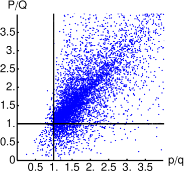
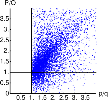
Figure 1: (Color online) Quantum-quantum YS effect vs quantum-classical YS effect for qubit systems. Left: the ratio $P/Q$ as a function of $p/q$ for $10^{4}$ randomly generated sets of states, measurements, and lurking variables. Right: the same plot for fixed values of the mixing parameters $\alpha=\beta=\pi/4$.

As it is apparent from the left plot, the two effects may occur independently, i.e. we may have $p<q$ when $P>Q$, and viceversa. For random settings, i.e. random states, measurements and lurking variables, the QQYS effect is more likely to occur than the corresponding CCYS effect. Upon generating a sample of $10^{4}$ random settings, we found QCYS effect without the QQYS one in about $0.97\%$ of cases, just the reverse in about $10.9\%$ of cases, and both effects in about $1.7\%$ of cases. The right plot refers to random initial states and measurements, and to lurking variables with equal mixing parameters $\cos^{2}\alpha=\cos^{2}\beta=\frac{1}{2}$. In this case, as mentioned before, the QCYS effect cannot occur for any measurement. On the other hand, upon considering quantum superpositions, we have that the QQYS effect occurs for a consistent fraction of the possible settings (about $14\%$). If we consider only projective measurements, the rates of occurrence of both the YS effects increases, but the overall picture is not qualitatively modified. Similar results are also obtained by considering three-dimensional quantum systems (qutrits).

4.1 Partial coherence and the generalized QQYS effect

Let us now assume that besides the complete mixture $\varrho_{\gamma}$, and the coherent superposition $|\psi_{\gamma}\rangle$, the system may be also prepared in partially coherent superpositions of the two initial states $|\psi_{j}\rangle$, i.e. we consider the general class of states $\varrho_{\lambda\gamma}=\lambda|\psi_{\gamma}\rangle\langle\psi_{\gamma}|+(1-\lambda)\varrho_{\gamma}$, where $\gamma=\alpha,\beta$, $0\leq\lambda\leq 1$. The family $\varrho_{\lambda\gamma}$ continuously connects the coherent superposition to the complete mixture, and we now address the occurrence of the corresponding generalized QQYS effect, which takes place, assuming again $p_{j}>q_{j}$, $j=1,2$, when we have $P_{\lambda}<Q_{\lambda}$, where $P_{\lambda}=\hbox{Tr}\left[\varrho_{\lambda\alpha}\,\Pi_{\scriptscriptstyle A}\right]=\lambda P+(1-\lambda)p$, $Q_{\lambda}=\hbox{Tr}\left[\varrho_{\lambda\beta}\,\Pi_{\scriptscriptstyle B}\right]=\lambda Q+(1-\lambda)q$. Using these expressions and introducing the threshold value

$$\lambda_{\rm th}=\left(1-\frac{P-Q}{p-q}\right)^{-1}\,,$$

one easily see that the QQYS effect persists in the range $\lambda\in(\lambda_{\rm th},1)$ if $p-q>P-Q$, or $\lambda\in(0,\lambda_{\rm th})$ if $p-q<P-Q$.

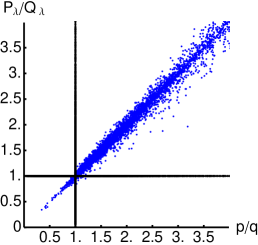
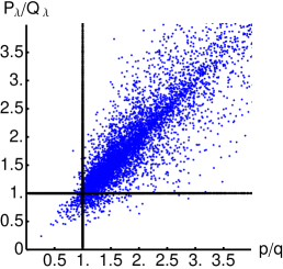
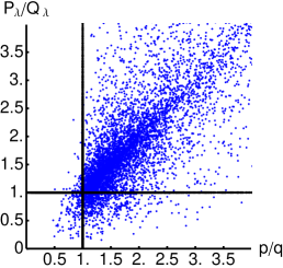
Figure 2: (Color online) Generalized quantum-quantum YS effect vs quantum-classical YS effect for qubit systems. The ratio $P_{\lambda}/Q_{\lambda}$ is shown as a function of $p/q$ for $10^{4}$ randomly generated sets of states, measurements, and lurking variables. From left to right: $\lambda=0.1,0.5,0.9$ respectively.

The transition from the QC to the QQ effect is illustrated in Fig. 2, where we show the ratio $P_{\lambda}/Q_{\lambda}$ as a function of the ratio $p/q$ for $10^{4}$ sets of randomly generated states, measurements and lurking variables (as in Fig. 1), and for different values of $\lambda$.

5 Conclusions

The Yule-Simpson is a paradigmatic paradoxical effect occurring in data aggregation in complex systems, and found applications in the physical description of, e.g. social processes [19], complex dynamics [20], and game theory [21]. In this communication, we have illustrated the occurrence of the YS effect in quantum measurements, where the lurking variables are coming either from the mixing or the superposition of quantum states. By analyzing low dimensional systems, we have found that the two effects may occur independently, and that the quantum-quantum YS effect is more likely to occur than the corresponding quantum-classical one for the same set of states and measurements. We have also discussed an example, illustrating the occurence of the quantum-classical YS effect in a decision problem involving quantum measurements.

Appendix A An example of YS effect: sex bias in graduate admissions

One of the best known real life examples of Simpson’s paradox occurred when the University of California, Berkeley was sued for bias against women who had applied for admission to graduate schools there [22]. The admission figures for the fall of 1973 showed that men applying were more likely than women to be admitted, and the difference was so large that it was unlikely to be due to statistical fluctuations. On the other hand, when examining the individual departments, it appeared that no department was significantly biased against women. In fact, most departments had a small but statistically significant bias in favor of women [3]. The explanation of the ”paradox” is relatively simple: the women tended to apply to competitive departments, with low rates of admission even among qualified applicants (such as in the English Department), whereas men tended to apply to less-competitive departments with high rates of admission among the qualified applicants (such as in engineering and chemistry), and overall this results in a smaller fraction of women admitted in total.

References

References

- [1] E. H. Simpson, J. Roy. Stat. Soc. B 13, 238 (1951).
- [2] C. R. Blyth J. Am. Stat. Ass. 67, 364 (1972).
- [3] P. J. Bickel, E. A. Hammel, J. W. O’Connell, Science 187, 398 (1975).
- [4] D. M. Messick, J. P. van de Geer, Psychol. Bull. 90, 582 (1981).
- [5] S. Ramanana-Rahary, M. Zitt, R. Rousseau, Scientometrics 79, 311 (2009).
- [6] J. S. Chuang, O. Rivoire, S. Leibler, Science 323, 272 (2009).
- [7] S. G. Baker, B. S. Kramer, J Women Health Gen-B 10, 867 (2001).
- [8] S. Lipovetsky, W. M. Conklin, Eur. J. Op. Res. 172, 334 (2006).
- [9] M. A. Hernan, D. Clayton, N. Keiding, Int. J. Epidem. 40, 780 (2011).
- [10] J. Aldrich, Stat. Sci. 10, 364 (1995).
- [11] D. R. Cox, W. Wermuth, J. Roy. Stat. Soc. B 65, 937 (2003).
- [12] J. M. R. Parrondo, G. P. Harmer, D. Abbott, Phys. Rev. Lett. 85, 5226 (2000).
- [13] J. Buceta, K. Lindenberg, J. M. R. Parrondo, Fluctuation Noise Lett. 2, L21 (2002).
- [14] R. J. Kay, N. F. Johnson, Phys. Rev. E 67, 056128 (2003).
- [15] R. D. Astumian, M. Bier, Phys. Rev. Lett. 72, 1766 (1994); R. D. Astumian, Am. J. Phys. 73, 178 (2005).
- [16] S. P. Gudder, Quantum probability, (Academic Press, Boston, 1988).
- [17] J. E. Cohen, Am. Stat. 40, 32 (1986).
- [18] P. Hadjicostas, Lin. Alg. Appl. 264, 475 (1997).
- [19] S. Galam, J. Stat. Phys. 61, 943 (1990).
- [20] J. Almeida, D. Peralta-Salas, M. Romera, Physica D 200, 124 (2005).
- [21] M. D. McDonnell, D. Abbot, Proc. Roy. Soc. A 465, 3309 (2009).
- [22] See more details and real figures at http://en.wikipedia.org/wiki/Simpson’s_paradox