Cycles and eigenvalues of sequentially growing random regular graphs

Abstract

Consider the sum of $d$ many i.i.d. random permutation matrices on $n$ labels along with their transposes. The resulting matrix is the adjacency matrix of a random regular (multi)-graph of degree $2d$ on $n$ vertices. It is known that the distribution of smooth linear eigenvalue statistics of this matrix is given asymptotically by sums of Poisson random variables. This is in contrast with Gaussian fluctuation of similar quantities in the case of Wigner matrices. It is also known that for Wigner matrices the joint fluctuation of linear eigenvalue statistics across minors of growing sizes can be expressed in terms of the Gaussian Free Field (GFF). In this article, we explore joint asymptotic (in $n$) fluctuation for a coupling of all random regular graphs of various degrees obtained by growing each component permutation according to the Chinese Restaurant Process. Our primary result is that the corresponding eigenvalue statistics can be expressed in terms of a family of independent Yule processes with immigration. These processes track the evolution of short cycles in the graph. If we now take $d$ to infinity, certain GFF-like properties emerge.

T1Supported in part by NSF Grant DMS-10-07563.

and

1 Introduction

We consider graphs that have labeled vertices and are regular, that is, every vertex has the same degree. We allow our graphs to have loops and multiple edges (such graphs are sometimes called multigraphs or pseudographs). Additionally, our graphs will be sparse in the sense that the degree will be negligible compared to the order. Every such graph has an associated adjacency matrix whose $(i,j)$th element is the number of edges between vertices $i$ and $j$, with loops counted twice. When the graph is randomly selected, the matrix is random, and we are interested in studying the eigenvalues of the resulting symmetric matrix. Note that, due to regularity, it does not matter whether we consider the eigenvalues of the adjacency or the Laplacian matrix.

The precise distribution of this random regular graph is somewhat ad hoc. We will use what is called the permutation model. Consider the permutation digraphs generated by $d$ many i.i.d. random permutations on $n$ labels. We remove the direction of the edge and collapse all these graphs on one another. This results in a $2d$-regular graph on $n$ vertices, denoted by $G(n,2d)$. At the matrix level this is given by adding all the $d$ permutation matrices and their transposes.

Our present work is an extension of the study of eigenvalue fluctuations carried out in DJPP . We are motivated by the recent work by Borodin on joint eigenvalue fluctuations of minors of Wigner matrices and the (massless or zero-boundary) Gaussian Free Field (GFF) Bor1 , Bor2 . Eigenvalues of minors are closely related to interacting particle systems Fer10 , FF10 , and the KPZ universality class of random surfaces BorFer . See JN for more on eigenvalues of minors of GUE and ANvM for those of Dyson’s Brownian motion.

Let us consider a particular but important case of Borodin’s result in Bor1 (single sequence, the entire $\mathbb{N}$). An $n\times n$ real symmetric Wigner matrix has i.i.d. upper triangular off-diagonal elements with four moments identical to the standard Gaussian. The diagonal elements are usually taken to be i.i.d. with mean zero variance two. Notice that every principal submatrix (called minors in this context) of a Wigner matrix is again a Wigner matrix of a smaller order. Thus, on some probability space one can construct an infinite order Wigner matrix $W$ whose $n\times n$ minor $W(n)$ is a Wigner matrix of order $n$.

Let $z$ be a complex number in the upper half plane $\mathbb{H}$. Define $y=|z|^{2}$ and $x=2\Re(z)$. Consider the minor $W(\lfloor ny\rfloor)$, and let $N(z)$ be the number of its eigenvalues that are greater than or equal to $\sqrt{n}x$. Define the height function

$$H_{n}(z):=\sqrt{\frac{\pi}{2}}N(z).$$ (1)

Then Borodin shows that $\{H_{n}(z)-EH_{n}(z),z\in\mathbb{H}\}$, viewed as distributions, converges in law to a generalized Gaussian process on $\mathbb{H}$ with a covariance kernel

$$C(z,w)=\frac{1}{2\pi}\ln\biggl{|}\frac{z-w}{z-\overline{w}}\biggr{|}.$$ (2)

The above is the covariance kernel for the GFF on the upper half plane.

An equivalent assertion is the following. Let $[n]$ denote the set of integers $\{1,2,\ldots,n\}$. Consider the Chebyshev polynomials of the first kind, $\{T_{n},n=0,1,2,\ldots\}$, on the interval $[-1,1]$. These polynomials are given by the identity $T_{n}(\cos(\theta))\equiv\cos(n\theta)$. We specialize Bor1 , Proposition 3, for the case of GOE ($\beta=1$). Fix $m$ positive real numbers $t_{1}<t_{2}<\cdots<t_{m}$. In the notation of Bor1 , we take $L=n$ and $B_{i}(n)=[\lfloor t_{i}n\rfloor]$. Then, for any positive integers $j_{1},j_{2},\ldots,j_{m}$, the random vector

$$\bigl{(}\mathop{\operatorname{tr}}T_{j_{i}}\bigl{(}W\bigl{(}\lfloor t_{i}n\rfloor\bigr{)}/2\sqrt{t_{i}n}\bigr{)}-\mathbf{E}\mathop{\operatorname{tr}}T_{j_{i}}\bigl{(}W\bigl{(}\lfloor t_{i}n\rfloor\bigr{)}/2\sqrt{t_{i}n}\bigr{)},i\in[m]\bigr{)}$$

converges in law, as $n$ tends to infinity, to a centered Gaussian vector. For $s\leq t$,

$$\quad\lim_{n\rightarrow\infty}\mathop{\operatorname{Cov}}\bigl{(}\mathop{\operatorname{tr}}T_{i}\bigl{(}W\bigl{(}\lfloor tn\rfloor\bigr{)}/2\sqrt{tn}\bigr{)},\mathop{\operatorname{tr}}T_{k}\bigl{(}W\bigl{(}\lfloor sn\rfloor\bigr{)}/2\sqrt{sn}\bigr{)}\bigr{)}=\delta_{ik}\frac{k}{2}\biggl{(}\frac{s}{t}\biggr{)}^{k/2},$$ (3)

which gives the covariance kernel of the limiting vector. In particular, all such covariances are zero when $i\neq k$. Note that the traces can be expressed as integrals of the height function of the corresponding submatrices. Thus, by approximating continuous compactly supported functions of $z$ by a function that is piecewise constant in $y$ and polynomial in $x$, one gets the kernel (2).

1.1 Main results

By a tower of random permutations, we mean a sequence of random permutations $(\pi^{(n)},n\in\mathbb{N})$ such that: [(ii)]

$\pi^{(n)}$ is a uniformly distributed random permutation of $[n]$ for each $n$, and

for each $n$, if $\pi^{(n)}$ is written as a product of cycles then $\pi^{(n-1)}$ is derived from $\pi^{(n)}$ by deletion of the element $n$ from its cycle. The stochastic process that grows $\pi^{(n)}$ from $\pi^{(n-1)}$ by sequentially inserting an element $n$ randomly is called the Chinese Restaurant Process (CRP). We will review the basic principles at a later section. In KOV and other related work, a sequence of permutations satisfying condition (ii) is called a virtual permutation, and the distribution on virtual permutations satisfying condition (i) is considered as a substitute for Haar measure on $S(\infty)$, the infinite symmetric group. This is used to study the representation theory of $S(\infty)$, with connections to random matrix theory. A recent extension of this idea is BNN .

Now suppose we construct a countable collection $\{\Pi_{d},d\in\mathbb{N}\}$ of towers of random permutations. We will denote the permutations in $\Pi_{d}$ by $\{\pi_{d}^{(n)},n\in\mathbb{N}\}$. Then it is possible to model every possible $G(n,2d)$ by adding the permutation matrices (and their transposes) corresponding to $\{\pi^{(n)}_{j},1\leq j\leq d\}$. In what follows, we will keep $d$ fixed and consider $n$ as a growing parameter. Thus, $G_{n}$ will represent $G(n,2d)$ for some fixed $d$. Here and later, $G_{0}$ will represent the empty graph. We construct a continuous-time version of this by inserting new vertices into $G_{n}$ with rate $n+1$. Formally, define independent times $T_{i}\sim\operatorname{Exp}(i)$, and let

$$M_{t}=\max\Biggl{\{}m\dvtx\sum_{i=1}^{m}T_{i}\leq t\Biggr{\}},$$

and define the continuous-time Markov chain $G(t)=G_{M_{t}}$. When $d=1$, this process is essentially just a continuous-time version of the CRP itself. Though this case is unusual compared to the rest—for example, $G(t)$ is likely to be disconnected when $d=1$ and connected when $d$ is larger—our results do still hold.

Our first result is about the process of short cycles in the graph process $G(t)$. By a cycle of length $k$ in a graph, we mean what is sometimes called a simple cycle: a walk in the graph that begins and ends at the same vertex, and that otherwise repeats no vertices. We will give a more formal definition in Section 2.2. Let $(C_{k}^{(s)}(t),k\in\mathbb{N})$ denote the number of cycles of various lengths $k$ that are present in $G(s+t)$. This process is not Markov, but nonetheless it converges to a Markov process (indexed by $t$) as $s$ tends to infinity.

To describe the limit, define

$$a(d,k)=\cases{(2d-1)^{k}-1+2d,&\quad$\mbox{when $k$ is even}$,\vspace*{2pt}\cr(2d-1)^{k}+1,&\quad$\mbox{when $k$ is odd}.$}$$

Consider the set of natural numbers $\mathbb{N}=\{1,2,\ldots\}$ with the measure

$$\mu(k)=\tfrac{1}{2}\bigl{[}a(d,k)-a(d,k-1)\bigr{]},\qquad k\in\mathbb{N},a(d,0):=0.$$

Consider a Poisson point process $\chi$ on $\mathbb{N}\times[0,\infty)$ with an intensity measure given on $\mathbb{N}\times(0,\infty)$ by the product measure $\mu\otimes\operatorname{Leb}$, where $\operatorname{Leb}$ is the Lebesgue measure, and with additional masses of $a(d,k)/2k$ on $(k,0)$ for $k\in\mathbb{N}$.

Let $\widetilde{P}_{x}$ denote the law of an one-dimensional pure-birth process on $\mathbb{N}$ given by the generator:

$$Lf(k)=k\bigl{(}f(k+1)-f(k)\bigr{)},\qquad k\in\mathbb{N},$$

starting from $x\in\mathbb{N}$. This is also known as the Yule process.

Suppose we are given a realization of $\chi$. For any atom $(k,y)$ of the countably many atoms of $\chi$, we start an independent process $(X_{k,y}(t),t\geq 0)$ with law $\widetilde{P}_{k}$. Define the random sequence

$${N}_{k}(t):=\sum_{(j,y)\in\chi\cap\{[k]\times[0,t]\}}1\bigl{\{}X_{j,y}(t-y)=k\bigr{\}}.$$

In other words, at time $t$, for every site $k$, we count how many of the processes that started at time $y\leq t$ at site $j\leq k$ are currently at $k$. Note that both $({N}_{k}(\cdot),k\in\mathbb{N})$ and $({N}_{k}(\cdot),k\in[K])$, for some $K\in\mathbb{N}$, are Markov processes, while $N_{k}(\cdot)$ for fixed $k$ is not.

Theorem 1.

As $s\to\infty$, the process $(C_{k}^{(s)}(t),k\in\mathbb{N},0\leq t<\infty)$ converges in law in $D_{\mathbb{R}^{\infty}}[0,\infty)$ to the Markov process $({N}_{k}(t),k\in\mathbb{N},0\leq t<\infty)$. The limiting process is stationary.

Remark 2.

In fact, the same argument used to prove Theorem 1 shows that the process $(C_{k}^{(s)}(t),-\infty<t<\infty)$ converges in law to the Markov process $({N}_{k}(t),-\infty<t<\infty)$ running in stationarity. The same conclusion holds for all the following theorems in this section.

We now explore the joint convergence across various $d$’s. Define $C_{d,k}^{(s)}(t)$ naturally, stressing the dependence on the parameter $d$.

Theorem 3.

There is a joint process convergence of $(C_{i,k}^{(s)}(t),k\in\mathbb{N},i\in[d],t\geq 0)$ to a limiting process $({N}_{i,k}(t),k\in\mathbb{N},i\in[d],t\geq 0)$. This limit is a Markov process whose marginal law for every fixed $d$ is described in Theorem 1. Moreover, for any $d\in\mathbb{N}$, the process $({N}_{d+1,k}(\cdot)-{N}_{d,k}(\cdot),k\in\mathbb{N})$ is independent of the process $({N}_{i,k}(\cdot),k\in\mathbb{N},i\in[d])$ and evolves as a Markov process. Its generator (defined on functions dependent on finitely many coordinates) is given by

$$Lf(x)=\sum_{k=1}^{\infty}kx_{k}\bigl{[}f(x+e_{k+1}-e_{k})-f(x)\bigr{]}+\sum_{k=1}^{\infty}\nu(d,k)\bigl{[}f(x+e_{k})-f(x)\bigr{]},$$

where $x$ is a nonnegative sequence, $(e_{k},k\in\mathbb{N})$ are the canonical orthonormal basis of $\ell^{2}$, and

$$\nu(d,k)=\tfrac{1}{2}\bigl{[}a(d+1,k)-a(d+1,k-1)-a(d,k)+a(d,k-1)\bigr{]}.$$

Remark 4.

Theorems 1 and 3 show an underlying branching process structure. We actually prove a more general decomposition where cycles are tracked by edge labels. The additive structure also imparts a natural intertwining relationship between the Markov operators. See CPY , Section 2 and DF90 , Bor1 .

We now focus on eigenvalues of $G(t)$. Note that there is no easy exact relationship between the eigenvalues of $G_{n}$ for various $n$ since the eigenvectors play a role in determining any such identity. In fact, the eigenvalues of $G_{n}$ and $G_{n+1}$ need not be interlaced. However, one can consider linear eigenvalue statistics for the graph $G(n,2d)$. That is, for any $d$-regular graph on $n$ vertices $G$ and function $f\dvtx\mathbb{R}\rightarrow\mathbb{R}$, define the random variable

$$\mathop{\operatorname{tr}}f(G):=\sum_{i=1}^{n}\hat{f}(\lambda_{i}),$$

where $\lambda_{1}\geq\cdots\geq\lambda_{n}$ are the eigenvalues of adjacency matrix of $G$ divided by $2(2d-1)^{1/2}$, and $\hat{f}$ is $f$ with its constant term adjusted [see (14) for the full definition]. The scaling is necessary to take a limit with respect to $d$.

By a polynomial basis we refer to a sequence of polynomials $\{f_{0}\equiv 1,f_{1},\break f_{2},\ldots\}$ such that $f_{k}$ is a polynomial of degree $k$ of a single argument over reals. In the statement below $[\infty]$ will refer to $\mathbb{N}$.

Theorem 5.

There exists a polynomial basis $\{f_{i},i\in\mathbb{N}\}$ (depending on $d$) such that for any $K\in\mathbb{N}\cup\{\infty\}$, the process $(\mathop{\operatorname{tr}}f_{k}(G(s+t)),k\in[K],t\geq 0)$ converges in law, as $s$ tends to infinity, to the Markov process $(N_{k}(t),k\in[K],t\geq 0)$ of Theorem 1. [The polynomials are given explicitly in (16).] Hence, for any polynomial $f$, the process $(\mathop{\operatorname{tr}}f(G(s+t)))$ converges to a linear combination of the coordinate processes of $(N_{k}(t),k\in\mathbb{N})$.

The Markov property is especially intriguing since, to the best of our knowledge, no similar property of eigenvalues of the standard Random Matrix ensembles is known. For the special case of minors of the Gaussian Unitary/Orthogonal Ensembles, the entire distribution of eigenvalues across minors of various sizes do satisfy a Markov property. However, this is facilitated by the known symmetry properties of the eigenvectors, and do not extend to other examples of Wigner matrices.

For our final result, we will take $d$ to infinity. We will make the following notational convention: for any polynomial $f$, we will denote the limiting process of $(\mathop{\operatorname{tr}}f(G(s+t)),t\geq 0)$ by $(\mathop{\operatorname{tr}}f(G(\infty+t)),t\geq 0)$. Recall that this process is a linear combination of $(N_{k}(t),k\in\mathbb{N},t\geq 0)$.

Theorem 6.

Let $\{T_{k},k\in\mathbb{N}\}$ denote the Chebyshev orthogonal polynomials of the first kind on $[-1,1]$. As $d$ tends to infinity, the collection of processes

$$\bigl{(}\mathop{\operatorname{tr}}T_{k}\bigl{(}G(\infty+t)\bigr{)}-\mathbf{E}\mathop{\operatorname{tr}}T_{k}\bigl{(}G(\infty+t)\bigr{)},t\geq 0,k\in\mathbb{N}\bigr{)}$$

converges weakly in $D^{\infty}[0,\infty)$ to a collection of independent Ornstein–Uhlenbeck processes $(U_{k}(t),t\geq 0,k\in\mathbb{N})$, running in equilibrium. Here the equilibrium distribution of $U_{k}$ is $N(0,k/2)$ and $U_{k}$ satisfies the stochastic differential equation

$$dU_{k}(t)=-kU_{k}(t)\,dt+k\,dW_{k}(t),\qquad t\geq 0,$$

and $(W_{k},k\in\mathbb{N})$ are i.i.d. standard one-dimensional Brownian motions.

Thus, the collection of random variables $(\mathop{\operatorname{tr}}T_{k}(G(\infty+t))-\break\mathbf{E}\mathop{\operatorname{tr}}T_{k}(G(\infty+t)))$, indexed by $k$ and $t$, converges as $d$ tends to infinity to a centered Gaussian process with covariance kernel given by

$$\lim_{d\rightarrow\infty}\mathop{\operatorname{Cov}}\bigl{(}\mathop{\operatorname{tr}}T_{i}\bigl{(}G(\infty+t)\bigr{)},\mathop{\operatorname{tr}}T_{k}\bigl{(}G(\infty+s)\bigr{)}\bigr{)}=\delta_{ik}\frac{k}{2}e^{k(s-t)}$$ (4)

for $s\leq t$.

A comparison of (4) with Borodin’s result (3) shows that the above limit captures a key property of the GFF covariance structure. The appearance of the exponential is merely due to a deterministic time-change of the process. A somewhat more detailed discussion can be found in the following section.

Remark 7.

A common model for random regular graphs is the configuration model or pairing model (see W for more information). The model is defined as follows: Start with $n$ buckets, each containing $d$ prevertices. Then, separate these $dn$ prevertices into pairs, choosing uniformly from every possible pairing. Finally, collapse each bucket into a single vertex, making an edge between one vertex and another if a prevertex in one bucket is paired with a prevertex in the other bucket. This model has the advantage that choosing a graph from it conditional on it containing no loops or parallel edges is the same as choosing a graph uniformly from the set of graphs without loops and parallel edges. The model also allows for graphs of odd degrees, unlike the permutation model.

It is possible to construct a process of growing random regular graphs similar to the one in this paper using a dynamic version of this model. Given some initial pairing of prevertices labeled $\{1,\ldots,dn\}$, extend it to a random pairing of $\{1,\ldots,dn+2\}$ by the following procedure: Choose $X$ uniformly from $\{1,\ldots,dn+1\}$. Pair $dn+2$ with $X$. If $X=dn+1$, leave the other pairs unchanged; if not, pair the previous partner of $X$ with $dn+1$. This is an analogue of the CRP in the setting of random pairings, in that if the initial pairing is uniformly chosen, then so is the extended one.

If $d$ is odd, we repeat this procedure a total of $d$ times to extend a random $d$-regular graph on $n$ vertices to have $n+2$ vertices (when $d$ is odd, the number of vertices in the graph must be even). When $d$ is even, repeat $d/2$ times to add one new vertex to a random graph. In this way, we can construct a sequence of growing random regular graphs. We believe that all the results of this paper hold in this model with minor changes, with similar proofs.

1.2 Existing literature

The study of the spectral properties of sparse regular random graphs is motivated by several different problems. These matrices do not fall within the purview of the standard techniques of Random Matrix Theory (RMT) due to their sparsity and lack of independence between entries. However, extensive simulations JMRR point to conjectures that these matrices still belong to the universality class of random matrices. For example, it is conjectured via simulations miller08 that the distribution of the second largest eigenvalue (in absolute value) is given by the Tracy–Widom distribution. In the physics literature, eigenvalues of random regular graphs have been considered as a toy model of quantum chaos Smi10 , OGS09 , OS10 . Simulations suggest that the eigenvalue spacing distribution has the same limit as that of the Wigner matrices. A limiting Gaussian wave character of eigenvectors have also been conjectured Elon08 , Elon09 , ES10 . Some fine properties of eigenvalues and eigenvectors can indeed be proved for a single permutation matrix; see W00 and BAD .

Somewhat complicating the matter is the fact that when the degree $d$ is kept fixed and we let $n$ go to infinity, several classical results about random matrix ensembles fail. A bit more elaboration on this point is needed. The two parameters in the ensemble of random graphs are the degree $d$ and the order $n$. In the permutation model it is possible to construct random regular graphs for every possible value of $(d,n)$ where $d$ is an even positive integer and $n$ is any positive integer. Hence, one can consider various kinds of limits of these parameters. We will refer as the diagonal limit the procedure of having a sequence of $(d,n)$ where both these parameters simultaneously go to infinity. To maintain sparsity, it is usually assumed that $d$ is at most poly-logarithmic in $n$. No lower bound on the growth rate of $d$ is assumed. However, results are often easier to prove when $d$ is kept fixed and we let $n$ go to infinity. Suppose for each $d$ one gets a limiting object (say a probability distribution); one can now take $d$ to infinity and explore limits of the sequence of these objects. We will refer to this procedure ($\lim_{d\rightarrow\infty}\lim_{n\rightarrow\infty}$) as the triangular limit. The triangular limit is often identical to the diagonal limit irrespective of the sequence through which the diagonal limit is taken, while maintaining sparsity. Moreover, these limiting statistics frequently match with those of the GOE ensemble and the real symmetric Wigner matrices. This is true, for example, for the empirical spectral distribution DP , TVW and fluctuations of smooth linear eigenvalue statistics DJPP .

Our present result is a triangular limit result. Let us first explain the connection with the massless GFF. We follow Definition 2.12 and the first example in Section 2.5 of SS07 . Consider the space of smooth real functions compactly supported on $\mathbb{H}$ with the Dirichlet inner product $\langle f,g\rangle=\int_{\mathbb{H}}\nabla f\cdot\nabla g\,dz$. Let $H$ be the completion of this pre-Hilbert space. The GFF can be thought of as a random distribution $h$ which associates with every $f\in H$ a mean zero Gaussian random variable $\langle h,f\rangle$ that is an $\mathbf{L}^{2}$ isometry in the sense that $\operatorname{Cov}(\langle h,f\rangle,\langle h,g\rangle)=\langle f,g\rangle$. Now, one can perform the integration of a function $f$ with $h$ by first integrating their traces over semicircular arcs of a fixed radius, and then a further integral over the radius. Over the semicircular arcs Fourier transforms (or Chebyshev Polynomials, for real functions) provide an orthogonal basis for this Gaussian field. As one parametrizes the radius properly, one obtains independent Ornstein–Uhlenbeck processes for each Chebyshev polynomial. Hence, these OU processes completely determine the GFF covariance structure. This explains the word “equivalent” on page 2, paragraph 4, and is the essence of the calculations done in Bor1 . See also Spohn98 for a similar formalism for Dyson’s Brownian motion on the circle.

One of the reasons why we cannot prove a full GFF convergence is that the parameters $d$ and $n$ behave independently of one another. The degree $d$ determines the support of the spectral distribution $[-2\sqrt{2d-1},2\sqrt{2d-1}]$, asymptotically independent of $n$. For Wigner matrices, the dimension itself determines the length of the spectral support. This results in the parametrization of (1). It should be possible to extend our results to a GFF convergence by either letting $d$ grow with $n$ in the graph, or, even by letting $d$ grow with time for the limiting Poisson structure in Theorem 1. Though we have not attempted this in the present article, we prove a result along these lines in naujasRE .

2 Preliminaries

2.1 A primer on the Chinese Restaurant Process

The CRP, introduced by Dubins and Pitman, is a particular example of a two parameter family of stochastic processes that constructs sequentially random exchangeable partitions of the positive integers via the cyclic decomposition of a random permutation. Our short description is taken from Pit , Section 3.1.

An initially empty restaurant has an unlimited number of circular tables numbered $1,2,\ldots,$ each capable of seating an unlimited number of customers. Customers numbered $1,2,\ldots$ arrive one by one and are seated at the tables according to the following plan. Person $1$ sits at table $1$. For $n\geq 1$ suppose that $n$ customers have already entered the restaurant, and are seated in some arrangement, with at least one customer at each of the tables $j$ for $1\leq j\leq k$ (say), where $k$ is the number of tables occupied by the first $n$ customers to arrive. Let customer $n+1$ choose with equal probability to sit at any of the following $n+1$ places: to the left of customer $j$ for some $1\leq j\leq n$, or alone at table $k+1$. Define $\pi^{(n)}\dvtx[n]\to[n]$ as the permutation whose cyclic decomposition is given by the tables; that is, if after $n$ customers have entered the restaurant, customers $i$ and $j$ are seated at the same table, with $i$ to the left of $j$, then $\pi^{(n)}(i)=j$, and if customer $i$ is seated alone at some table then $\pi^{(n)}(i)=i$. The sequence $(\pi^{(n)})$ then has features (i) and (ii) mentioned in the first paragraph of Section 1.1.

2.2 Combinatorics on words

The graph $G_{n}$, formed from the independent permutations $\pi^{(n)}_{1},\ldots,\pi^{(n)}_{d}$, can be considered as a directed, edge-labeled graph in a natural way. For convenience, drop superscripts and let $\pi_{l}=\pi^{(n)}_{l}$. If $\pi_{l}(i)=j$, then by definition $G_{n}$ contains an edge between $i$ to $j$. When convenient, we consider this edge to be directed from $i$ to $j$ and to be labeled by $\pi_{l}$.

Consider a walk on $G_{n}$, viewed in this way, and imagine writing down the label of each edge as it is traversed, putting $\pi_{i}$ or $\pi_{i}^{-1}$ according to the direction we walk over the edge. We call a walk closed if it starts and ends at the same vertex, and we call a closed walk a cycle it never visits a vertex twice (besides the first and last one), and it never traverses an edge more than once in either direction. Thus the word $w=w_{1}\cdots w_{k}$ formed as a cycle is traversed is cyclically reduced, that is, $w_{i}\neq w_{i+1}^{-1}$ for all $i$, considering $i$ modulo $k$. For example, following an edge and then immediately backtracking does not form a $2$-cycle, and the word formed by this walk is $\pi_{i}\pi_{i}^{-1}$ or $\pi_{i}^{-1}\pi_{i}$ for some $i$, which is not cyclically reduced. We consider two cycles equivalent if they are both walks on an identical set of edges; that is, we ignore the starting vertex and the direction of the walk.

Figure 1: A cycle whose word is the equivalence class of $\pi_{2}\pi_{1}^{-1}\pi_{2}\pi_{1}\pi_{2}\pi_{3}^{-1}$ in $\mathcal{W}_{6}/D_{12}$.

Let $\mathcal{W}_{k}$ denote the set of cyclically reduced words of length $k$. We would like to associate each $k$-cycle in $G_{n}$ with the word in $\mathcal{W}_{k}$ formed by the above procedure, but since we can start the walk at any point in the cycle and walk in either of two directions, there are actually up to $2k$ different words that could be formed by it. Thus, we identify elements of $\mathcal{W}_{k}$ that differ only by rotation and inversion (e.g., $\pi_{1}\pi_{2}^{-1}\pi_{1}\pi_{2}$ and $\pi_{1}^{-1}\pi_{2}\pi_{1}^{-1}\pi_{2}^{-1}$) and denote the resulting set by $\mathcal{W}_{k}/D_{2k}$, where $D_{2k}$ is the dihedral group acting on the set $\mathcal{W}_{k}$ in the natural way.

Definition 8 ((Properties of words)).

For any $k$-cycle in $G_{n}$, the element of $\mathcal{W}_{k}/D_{2k}$ given by walking around the cycle is called the word of the cycle (see Figure 1). For any word $w$, let $|w|$ denote the length of $w$. Let $h(w)$ be the largest number $m$ such that $w=u^{m}$ for some word $u$. If $h(w)=1$, we call $w$ primitive. For any $w\in\mathcal{W}_{k}$, the orbit of $w$ under the action of $D_{2k}$ contains $2k/h(w)$ elements, a fact which we will frequently use. Let $c(w)$ denote the number of pairs of double letters in $w$, that is, the number of integers $i$ modulo $|w|$ such that $w_{i}=w_{i+1}$. If $w$ has length 1, then we define $c(w)=0$. For example, $c(\pi_{1}\pi_{1}\pi_{2}^{-1}\pi_{2}^{-1}\pi_{1})=3$. We will also consider $|\cdot|$, $h(\cdot)$, and $c(\cdot)$ as functions on $\mathcal{W}_{k}/D_{2k}$, since they are invariant under cyclic rotation and inversion.

To more easily refer to words in $\mathcal{W}_{k}/D_{2k}$, choose some canonical representative $w_{1}\cdots w_{k}\in\mathcal{W}_{k}$ for every $w\in\mathcal{W}_{k}/D_{2k}$. Based on this, we will often think of elements of $\mathcal{W}_{k}/D_{2k}$ as words instead of equivalence classes, and we will make statements about the $i$th letter of a word in $\mathcal{W}_{k}/D_{2k}$. For $w=w_{1}\cdots w_{k}\in\mathcal{W}_{k}/D_{2k}$, let $w^{(i)}$ refer to the word in $\mathcal{W}_{k+1}/D_{2k+2}$ given by $w_{1}\cdots w_{i}w_{i}w_{i+1}\cdots w_{k}$. We refer to this operation as doubling the $i$th letter of $w$. A related operation is to halve a pair of double letters, for example producing $\pi_{1}\pi_{2}\pi_{3}\pi_{4}$ from $\pi_{1}\pi_{2}\pi_{3}\pi_{4}\pi_{1}$. (Since we apply these operations to words identified with their rotations, we do not need to be specific about which letter of the pair is deleted.) The following technical lemma underpins most of our combinatorial calculations.

Lemma 9.

Let $u\in\mathcal{W}_{k}/D_{2k}$ and $w\in\mathcal{W}_{k+1}/D_{2k+2}$. Suppose that $a$ letters in $u$ can be doubled to form $w$, and $b$ pairs of double letters in $w$ can be halved to form $u$. Then

$$\frac{a}{h(u)}=\frac{b}{h(w)}.$$

Remark 10.

At first glance, one might expect that $a=b$. The example $u=\pi_{1}\pi_{2}\pi_{1}\pi_{1}\pi_{2}$ and $w=\pi_{1}\pi_{1}\pi_{2}\pi_{1}\pi_{1}\pi_{2}$ shows that this is wrong, since only one letter in $u$ can be doubled to give $w$, but two different pairs in $w$ can be halved to give $u$.

Let $\mathop{\operatorname{Orb}}(u)$ and $\mathop{\operatorname{Orb}}(w)$ denote the orbits of $u$ and $w$ under the action of the dihedral group in $\mathcal{W}_{k}$ and $\mathcal{W}_{k+1}$, respectively. When we speak of halving a pair of letters in a word in $\mathop{\operatorname{Orb}}(w)$, always delete the second of the two letters (e.g., $\pi_{1}\pi_{2}\pi_{1}$ becomes $\pi_{1}\pi_{2}$, not $\pi_{2}\pi_{1}$). When we double a letter in a word in $\mathop{\operatorname{Orb}}(u)$, put the new letter after the doubled letter (e.g., doubling the second letter of $\pi_{1}\pi_{2}^{-1}$ gives $\pi_{1}\pi_{2}^{-1}\pi_{2}^{-1}$, not $\pi_{2}^{-1}\pi_{1}\pi_{2}^{-1}$).

For each of the $2k/h(u)$ words in $\mathop{\operatorname{Orb}}(u)$, there are $a$ doubling operations yielding a word in $\mathop{\operatorname{Orb}}(w)$. For each of the $(2k+2)/h(w)$ words in $\mathop{\operatorname{Orb}}(w)$, there are $b$ halving operations yielding a word in $\mathop{\operatorname{Orb}}(u)$. For every halving operation on a word in $\mathop{\operatorname{Orb}}(w)$, there is a corresponding doubling operation on a word in $\mathop{\operatorname{Orb}}(u)$ and vice versa, except for halving operations that straddle the ends of the word, as in $\pi_{1}\pi_{2}\pi_{1}$. There are $2b/h(w)$ of these, giving us

$$\frac{2ka}{h(u)} = \frac{(2k+2)b}{h(w)}-\frac{2b}{h(w)}$$

$$= \frac{2kb}{h(w)},$$

and the lemma follows from this.

Let $\mathcal{W}^{\prime}=\bigcup_{k=1}^{\infty}\mathcal{W}_{k}/D_{2k}$, and let $\mathcal{W}^{\prime}_{K}=\bigcup_{k=1}^{K}\mathcal{W}_{k}/D_{2k}$. We will use the previous lemma to prove the following technical property of the $c(\cdot)$ statistic.

Lemma 11.

In the vector space with basis $\{q_{w}\}_{w\in\mathcal{W}_{K}^{\prime}}$,

$$\sum_{w\in\mathcal{W}_{K-1}^{\prime}}\sum_{i=1}^{|w|}\frac{1}{h(w)}q_{w^{(i)}}=\sum_{w\in\mathcal{W}_{K}^{\prime}}\frac{c(w)}{h(w)}q_{w}.$$

Fix some $w\in\mathcal{W}_{k}/D_{2k}$, and let $a(u)$ denote the number of letters of $u$ that can be doubled to give $w$, for any $u\in\mathcal{W}_{k-1}/D_{2k-2}$. We need to prove that

$$\sum_{u\in\mathcal{W}_{k-1}/D_{2k-2}}\frac{a(u)}{h(u)}=\frac{c(w)}{h(w)}.$$

Let $b(u)$ be the number of pairs in $w$ that can be halved to give $u$. By Lemma 9,

$$\sum_{u\in\mathcal{W}_{k-1}/D_{2k-2}}\frac{a(u)}{h(u)}=\sum_{u\in\mathcal{W}_{k-1}/D_{2k-2}}\frac{b(u)}{h(w)},$$

and $\sum_{u\in\mathcal{W}_{k-1}/D_{2k-2}}b(u)=c(w)$.

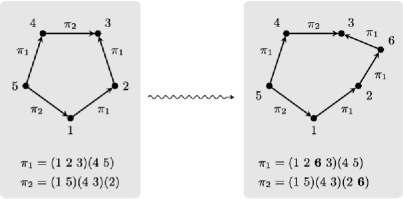
Figure 2: The vertex $6$ is inserted between vertices $2$ and $3$ in $\pi_{1}$, causing the above cycle to grow.

3 The process limit of the cycle structure

As the graph $G(t)$ grows, new cycles form, which we can classify into two types. Suppose a new vertex numbered $n$ is inserted at time $t$, and this insertion creates a new cycle. If the edges entering and leaving vertex $n$ in the new cycle have the same edge label, then the new cycle has “grown” from a cycle with one fewer vertex, as in Figure 2. If the edges entering and leaving $n$ in the cycle have different labels, then the cycle has formed “spontaneously” as in Figure 3, rather than growing from a smaller cycle. This classification will prove essential in understanding the evolution of cycles in $G(t)$.

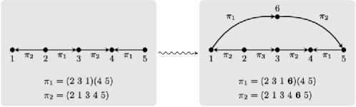
Figure 3: A cycle forms “spontaneously” when the vertex $6$ is inserted into the graph.

Once a cycle comes into existence in $G(t)$, it remains until a new vertex is inserted into one of its edges. Typically, this results in the cycle growing to a larger cycle, as in Figure 2. If a new vertex is simultaneously inserted into multiple edges of the same cycle, the cycle is instead split into smaller cycles as in Figure 4. These new cycles are spontaneously formed, according to the classification of new cycles given in the previous paragraph. Tracking the evolution of these smaller cycles in turn, we see that as the graph evolves, a cycle grows into a cluster of overlapping cycles. However, it will follow from Proposition 19 that for short cycles, this behavior is not typical. Thus in our limiting object, cycles will grow only into larger cycles.

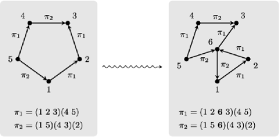
Figure 4: The vertex $6$ is inserted into the cycle in two different places in the same step, causing the cycle to split in two. Note that each new cycle would be classified as spontaneously formed.

3.1 Heuristics for the limiting process

We give some estimates that will motivate the definition of the limiting process in Section 3.2. This section is entirely motivational, and we will not attempt to make anything rigorous.

Suppose that vertex $n$ is inserted into $G(t)$ at some time $t$. First, we consider the rate that cycles form spontaneously with some word $w\in\mathcal{W}_{k}/D_{2k}$. There are $2k/h(w)$ words in the orbit of $w$ under the action of $D_{2k}$, and out of these, $2(k-c(w))/h(w)$ have nonequal first and last letters. For each such word $u=u_{1}\cdots u_{k}$, we can give a walk on the graph by starting at vertex $n$ and following the edges indicated by $u$, going from $n$ to $u_{1}(n)$ to $u_{2}(u_{1}(n))$ and so on. If this walk happens to be a cycle, the condition $u_{1}\neq u_{k}$ implies that it would be spontaneously formed.

In a short interval $\Delta t$ when $G(t)$ has $n-1$ vertices, the probability that vertex $n$ is inserted is about $n\Delta t$. For any word $u$, the walk from vertex $n$ generated by $u$ is a cycle with probability approximately $1/n$, since after applying the random permutations $u_{1},\ldots,u_{k}$ in turn, we will be left at an approximately uniform random vertex. Any new spontaneous cycle formed with word $w$ will be counted by one of these walks, with $u$ in the orbit of $w$, and it will be counted again by the walk generated by $u_{k}^{-1}\cdots u_{1}^{-1}$. The expected number of spontaneous cycles formed in a short interval $\Delta t$ is then approximately

$$\frac{1}{h(w)}\bigl{(}k-c(w)\bigr{)}\frac{n\Delta t}{n}=\frac{1}{h(w)}\bigl{(}k-c(w)\bigr{)}\Delta t.$$

Thus, we will model the spontaneous formation of cycles with word $w$ by a Poisson process with rate $(k-c(w))/h(w)$.

Next, we consider how often a cycle with word $w\in\mathcal{W}_{k}$ grows into a larger cycle. Suppose that $G(t)$ has $n-1$ vertices, and that it contains a cycle of the form

When vertex $n$ is inserted into the graph, the probability that it is inserted after $s_{i-1}$ in permutation $w_{i}$ is $1/n$. Thus, after a spontaneous cycle with word $w$ has formed, we can model the evolution of its word as a continuous-time Markov chain where each letter is doubled with rate one.

3.2 Formal definition of the limiting process

Consider the measure $\mu$ on $\mathcal{W}^{\prime}$ given by

$$\mu(w)=\frac{|w|-c(w)}{h(w)}.$$

Consider a Poisson point process $\chi$ on $\mathcal{W}^{\prime}\times[0,\infty)$ with an intensity measure given by the product measure $\mu\otimes\operatorname{Leb}$, where $\operatorname{Leb}$ refers to the Lebesgue measure. Each atom $(w,t)$ of $\chi$ represents a new spontaneous cycle with word $w$ formed at time $t$.

Now, we define a continuous-time Markov chain on the countable space $\mathcal{W}^{\prime}$ governed by the following rates: From state $w\in\mathcal{W}_{k}/D_{2k}$, jump with rate one to each of the $k$ words in $\mathcal{W}_{k+1}/D_{2k+2}$ obtained by doubling a letter of $w$. If a word can be formed in more than one way by doubling a letter in $w$, then it receives a correspondingly higher rate. For example, from $w=\pi_{1}\pi_{1}\pi_{2}$, the chain jumps to $\pi_{1}\pi_{1}\pi_{1}\pi_{2}$ with rate two and to $\pi_{1}\pi_{1}\pi_{2}\pi_{2}$ with rate one. Let $\widetilde{P}_{w}$ denote the law of this process started from $w\in\mathcal{W}^{\prime}$.

Suppose we are given a realization of $\chi$. For any atom $(w,s)$ of the countably many atoms of $\chi$, we start an independent process $(X_{w,s}(t),t\geq 0)$ with law $\widetilde{P}_{w}$. Define the stochastic process

$$N_{w}{({t})}:=\mathop{\sum_{(u,s)\in\chi}}_{s\leq t}1\bigl{\{}X_{u,s}(t-s)=w\bigr{\}}.$$

Interpreting these processes as in the previous section, $N_{w}{({t})}$ counts the number of cycles formed spontaneously at time $s$ that have grown to have word $w$ at time $t$.

The fact that the process exists is obvious since one can define the countably many independent Markov chains on a suitable product space. The following lemma establishes some of its key properties.

Lemma 12.

Recall that $\mathcal{W}_{L}^{\prime}=\bigcup_{k=1}^{L}\mathcal{W}_{k}/D_{2k}$. We have the following conclusions: [(iii)]

For any $L\in\mathbb{N}$, the stochastic process $\{(N_{w}{({t})},w\in\mathcal{W}_{L}^{\prime}),t\geq 0\}$ is a time-homogeneous Markov process with respect to its natural filtration, with RCLL paths.

Recall that for $w\in\mathcal{W}_{k}/D_{2k}$, the element $w^{(i)}\in\mathcal{W}_{k+1}/D_{2k+2}$ is the word formed by doubling the $i$th letter of $w$. The generator for the Markov process $\{(N_{w}{({t})},w\in\mathcal{W}_{L}^{\prime}),t\geq 0\}$ acts on $f$ at $x=(x_{w},w\in\mathcal{W}_{L}^{\prime})$ by

$$\mathcal{L}f(x) = \sum_{w\in\mathcal{W}_{L}^{\prime}}\sum_{i=1}^{|w|}x_{w}\bigl{[}f(x-e_{w}+e_{w^{(i)}})-f(x)\bigr{]}$$

$${}+\sum_{w\in\mathcal{W}^{\prime}_{L}}\frac{|w|-c(w)}{h(w)}\bigl{[}f(x+e_{w})-f(x)\bigr{]},$$

where $e_{w}$ is the canonical basis vector equal to one at entry $w$ and equal to zero everywhere else. For a word $u$ of length greater than $L$, take $e_{u}=0$.

The product measure of $\operatorname{Poi}(1/h(w))$ over all $w\in\mathcal{W}_{L}^{\prime}$ is the unique invariant measure for this Markov process.

Conclusion (i) follows from construction, as does conclusion (ii). To prove conclusion (iii), we start by the fundamental identity of the Poisson distribution: if $X\sim\operatorname{Poi}(\lambda)$, then for any function $f$, we have

$$\mathbf{E}Xg(X)=\lambda\mathbf{E}g(X+1).$$ (5)

We need to show that if the coordinates of $X=(X_{w},w\in\mathcal{W}^{\prime}_{L})$ are independent Poisson random variables with $\mathbf{E}X_{w}=1/h(w)$, then

$$\mathbf{E}\mathcal{L}f(X)=0.$$ (6)

Since the process is an irreducible Markov chain on countable state space, the existence of one invariant distribution shows that the chain is positive recurrent and that the invariant distribution is unique.

To argue (6), we will repeatedly apply identity (5) to functions $g$ constructed from $f$ by keeping all but one coordinate fixed. Thus, for any $w\in\mathcal{W}_{L}^{\prime}$ and $1\leq i\leq|w|$, we condition on all $X_{u}$ with $u\neq w$ and hold those coordinates of $f$ fixed to obtain,

$$\mathbf{E}X_{w}f(X-e_{w}+e_{w^{(i)}})=\frac{1}{h(w)}\mathbf{E}f(X+e_{w^{(i)}})$$

taking $e_{w^{(i)}}=0$ when $|w|=L$. In the same way,

$$\mathbf{E}X_{w}f(X)=\frac{1}{h(w)}\mathbf{E}f(X+e_{w}).$$

By these two equalities,

$$\mathbf{E}\sum_{w\in\mathcal{W}_{L}^{\prime}}\sum_{i=1}^{|w|}X_{w}\bigl{[}f(X-e_{w}+e_{w^{(i)}})-f(X)\bigr{]}$$

$$\qquad=\sum_{w\in\mathcal{W}_{L}^{\prime}}\sum_{i=1}^{|w|}\frac{1}{h(w)}\mathbf{E}\bigl{[}f(X+e_{w^{(i)}})-f(X+e_{w})\bigr{]}$$

$$\qquad=\sum_{w\in\mathcal{W}_{L-1}^{\prime}}\sum_{i=1}^{|w|}\frac{1}{h(w)}\mathbf{E}f(X+e_{w^{(i)}})+\sum_{w\in\mathcal{W}_{L}/D_{2L}}\frac{|w|}{h(w)}\mathbf{E}f(X)$$

$$\qquad\quad{}-\sum_{w\in\mathcal{W}^{\prime}_{L}}\frac{|w|}{h(w)}\mathbf{E}f(X+e_{w}).$$

Specializing Lemma 11 to $q_{w}=\mathbf{E}f(X+e_{w})$, the first sum is

$$\sum_{w\in\mathcal{W}_{L-1}^{\prime}}\sum_{i=1}^{|w|}\frac{1}{h(w)}\mathbf{E}f(X+e_{w^{(i)}})=\sum_{w\in\mathcal{W}^{\prime}_{L}}\frac{c(w)}{h(w)}\mathbf{E}f(X+e_{w}),$$

which gives us

$$\mathbf{E}\sum_{w\in\mathcal{W}_{L}^{\prime}}\sum_{i=1}^{|w|}X_{w}\bigl{[}f(X-e_{w}+e_{w^{(i)}})-f(X)\bigr{]}$$

$$\qquad=\sum_{w\in\mathcal{W}^{\prime}_{L}}\frac{c(w)-|w|}{h(w)}\mathbf{E}f(X+e_{w})+\sum_{w\in\mathcal{W}_{L}/D_{2L}}\frac{|w|}{h(w)}\mathbf{E}f(X).$$

All that remains in proving (6) is to show that

$$\sum_{w\in\mathcal{W}_{L}^{\prime}}\frac{|w|-c(w)}{h(w)}=\sum_{w\in\mathcal{W}_{L}/D_{2L}}\frac{|w|}{h(w)}.$$

Specializing Lemma 11 to $q_{w}=1$ shows that $\sum_{w\in\mathcal{W}_{L}^{\prime}}c(w)/h(w)=\break\sum_{w\in\mathcal{W}_{L-1}^{\prime}}|w|/{h(w)}$. Thus,

$$\sum_{w\in\mathcal{W}_{L}^{\prime}}\frac{|w|-c(w)}{h(w)} = \sum_{w\in\mathcal{W}_{L}^{\prime}}\frac{|w|}{h(w)}-\sum_{w\in\mathcal{W}_{L-1}^{\prime}}\frac{|w|}{h(w)}$$

$$= \sum_{w\in\mathcal{W}_{L}/D_{2L}}\frac{|w|}{h(w)},$$

establishing (6) and completing the proof. From now on, we will consider the process $(N_{w}{({t})},k\in\mathbb{N},t\geq 0)$ to be running under stationarity, that is, with marginal distributions given by conclusion (iii) of the last lemma. This process is easily constructed as described above, but with additional point masses of weight $1/h(w)$ for each $w\in\mathcal{W}^{\prime}$ at $(w,0)$ added to the intensity measure of $\chi$, thus giving us the correct distribution at time zero.

3.3 Time-reversed processes

Fix some time $T>0$. We define the time-reversal $\overleftarrow{N}_{w}{({t})}:=N_{w}{({T-t})}$ for $0\leq t\leq T$.

Lemma 13.

For any fixed $L\in\mathbb{N}$, the process $\{(\overleftarrow{N}_{w}{({t})},w\in\mathcal{W}^{\prime}_{L}),\break 0\leq t\leq T\}$ is a time-homogenous Markov process with respect to the natural filtration. A trivial modification at jump times renders RCLL paths. The transition rates of this chain are given as follows. Let $u\in\mathcal{W}_{k-1}/D_{2k-1}$ and $w\in\mathcal{W}_{k}/D_{2k}$, and suppose that $u$ can be obtained from $w$ by halving $b$ different pairs. Let $x=(x_{w},w\in\mathcal{W}^{\prime}_{L})$. [(iii)]

The chain jumps from $x$ to $x+e_{u}-e_{w}$ with rate $bx_{w}$.

The chain jumps from $x$ to $x-e_{w}$ with rate $(k-c(w))x_{w}$.

If $w\in\mathcal{W}_{L}/D_{2L}$, then the chain jumps from $x$ to $x+e_{w}$ with rate $L/h(w)$.

Any Markov process run backwards under stationarity is Markov. If the chain has transition rate $r(x,y)$ from states $x$ to $y$, then the transition rate of the backwards chain from $x$ to $y$ is $r(y,x)\nu(y)/\nu(x)$, where $\nu$ is the stationary distribution. We will let $\nu$ be the stationary distribution from Lemma 12(iii) and calculate the transition rates of the backwards chain, using the rates given in Lemma 12(ii).

Let $a$ denote the number of letters in $u$ that give $w$ when doubled. The transition rate of the original chain from $x+e_{u}-e_{w}$ to $x$ is $a(x_{u}+1)$, so the transition rate of the backwards chain from $x$ to $x+e_{u}-e_{w}$ is

$$a(x_{u}+1)\frac{\nu(x+e_{k-1,c-1}-e_{k,c})}{\nu(x)}=\frac{ah(w)x_{w}}{h(u)},$$

and this is equal to $bx_{w}$ by Lemma 9. A similar calculation shows that the transition rate from $x$ to $x-e_{w}$ is

$$\frac{(k-c(w))\nu(x-e_{w})}{h(w)\nu(x)}=\bigl{(}k-c(w)\bigr{)}x_{w},$$

proving (ii). The transition rate from $x$ to $x+e_{w}$ for $w\in\mathcal{W}_{L}/D_{2L}$ is

$$\frac{\nu(x+e_{w})}{\nu(x)}(x_{w}+1)L=\frac{L}{h(w)},$$

which completes the proof. By definition,

$$\overleftarrow{N}_{w}{({t})}=\mathop{\sum_{(u,s)\in\chi}}_{s\leq T-t}1\bigl{\{}X_{u,s}(T-t-s)=w\bigr{\}}.$$

We will modify this slightly to define the process

$$\overleftarrow{M}_{w}{({t})}:=\mathop{\sum_{(u,s)\in\chi}}_{s\leq T-t}1\bigl{\{}X_{u,s}(T-t-s)=w\mbox{ and }\bigl{|}X_{u,s}(T-s)\bigr{|}\leq L\bigr{\}}.$$

The idea is that $\overleftarrow{M}_{w}{({t})}$ is the same as $\overleftarrow{N}_{w}{({t})}$, except that it does not count cycles at time $t$ that had more than $L$ vertices at time zero. The process $(\overleftarrow{M}_{w}{({t})},w\in\mathcal{W}_{L}^{\prime})$ is a Markov chain with the same transition rates as $(\overleftarrow{N}_{w}{({t})},w\in\mathcal{W}_{L}^{\prime})$, except that it does not jump from $x$ to $x+e_{w}$ for $w\in\mathcal{W}_{L}/D_{2L}$. These two chains also have the same initial distribution, but $(\overleftarrow{M}_{w}{({t})},w\in\mathcal{W}_{L}^{\prime})$ is not stationary (in fact, it is eventually absorbed at zero).

4 Process convergence

Recall that $C_{k}^{(s)}(t)$ is the number of cycles of length $k$ in the graph $G(s+t)$, defined on page 1.1. For $w\in\mathcal{W}^{\prime}$, let $C_{w}^{(s)}(t)$ be the number of cycles in $G(s+t)$ with word $w$. We will prove that $(C_{w}^{(s)}(\cdot),w\in\mathcal{W}^{\prime})$ converges to a distributional limit, from which the convergence of $(C_{k}^{(s)}(\cdot),k\in\mathbb{N})$ will follow. The proof depends on knowing the limiting marginal distribution of $C_{w}^{(s)}(t)$. We provide this and more in the following theorem, which should be of independent interest.

Theorem 14.

Let $G_{n}=G(n,2d)$, a $2d$-regular random graph on $n$ vertices from the permutation model. For any $k$, let $\mathcal{I}_{k}$ be the set of all cycles of length $k$ on the complete graph $K_{n}$ with edge labels that form a cyclically reduced word; these are the possible $k$-cycles that might appear in $G_{n}$. Let $\mathcal{I}=\bigcup_{k=1}^{r}\mathcal{I}_{k}$ for some integer $r$.

For any cycle $\alpha\in\mathcal{I}$, let $I_{\alpha}=1\{G_{n}\mbox{ contains }\alpha\}$, and let $\mathbf{I}=(I_{\alpha},\alpha\in\mathcal{I})$. Let $\mathbf{Z}=(Z_{\alpha},\alpha\in\mathcal{I})$ be a vector whose coordinates are independent Poisson random variables with $\mathbf{E}Z_{\alpha}=1/[n]_{k}$ for $\alpha\in\mathcal{I}_{k}$. Then for all $d\geq 2$ and $n,r\geq 1$,

$$d_{\mathrm{TV}}(\mathbf{I},\mathbf{Z})\leq\frac{c(2d-1)^{2r-1}}{n}$$

for some absolute constant $c$, where $d_{\mathrm{TV}}(X,Y)$ denotes the total variation distance between the laws of $X$ and $Y$.

Corollary 15.

Let $\{Z_{w},w\in\mathcal{W}^{\prime}_{K}\}$ be a family of independent Poisson random variables with $\mathbf{E}Z_{w}=1/h(w)$. For any fixed integer $K$ and $d\geq 1$, [(ii)]

as $t\to\infty$,

$$\bigl{(}C_{w}(t),w\in\mathcal{W}^{\prime}_{K}\bigr{)}\,{\buildrel\mathcal{L}\over{\longrightarrow}}\,\bigl{(}Z_{w},w\in\mathcal{W}^{\prime}_{K}\bigr{)};$$

as $t\to\infty$, the probability that there exist two cycles of length $K$ or less sharing a vertex in $G(t)$ approaches zero.

We give the proofs in the Appendix, along with some further discussion. Now, we turn to the convergence of the processes.

Theorem 16.

The process $(C_{w}^{(s)}(\cdot),w\in\mathcal{W}^{\prime})$ converges in law as $s\to\infty$ to $(N_{w}{({\cdot})},w\in\mathcal{W}^{\prime})$.

The main difficulty in turning the intuitive ideas of Section 3.1 into an actual proof is that $(C_{w}^{(s)}(t),w\in\mathcal{W}^{\prime})$ is not Markov. We now sketch how we evade this problem. We will run our chain backwards, defining $\overleftarrow{G}_{s}(t)=G(s+T-t)$ for some fixed $T>0$. Then, we ignore all of $\overleftarrow{G}_{s}(0)$ except for the subgraph consisting of cycles of size $L$ and smaller, which we will call ${\overleftarrow{\Gamma}{}_{s}(0)}$. The graph ${\overleftarrow{\Gamma}_{s}(t)}$ is the evolution of this subgraph as time runs backward, ignoring the rest of $\overleftarrow{G}_{s}(t)$. Then, we consider the number of cycles with word $w$ in ${\overleftarrow{\Gamma}_{s}(t)}$, which we call $\phi_{w}({\overleftarrow{\Gamma}_{s}(t)})$. Choose $K\ll L$. Then $\phi_{w}({\overleftarrow{\Gamma}_{s}(t)})$ is likely to be the same as $C_{w}^{(s)}(T-t)$ for any word $w$ with $|w|\leq K$. The remarkable fact that makes $\phi_{w}({\overleftarrow{\Gamma}_{s}(t)})$ possible to analyze is that if ${\overleftarrow{\Gamma}_{s}(0)}$ consists of disjoint cycles, then $(\phi_{w}({\overleftarrow{\Gamma}_{s}(t)}),w\in\mathcal{W}^{\prime}_{L})$ is a Markov chain governed by the same transition rates as $(\overleftarrow{M}_{w}{({t})},w\in\mathcal{W}^{\prime}_{L})$.

Another important idea of the proof is to ignore the vertex labels in $\overleftarrow{G}_{s}(t)$, so that we do not know in what order the vertices will be removed. Thus, we can view $\overleftarrow{G}_{s}(t)$ as a Markov chain with the following description: Assign each vertex an independent $\operatorname{Exp}(1)$ clock. When the clock of vertex $v$ goes off, remove it from the graph, and patch together the $\pi_{i}$-labeled edges entering and leaving $v$ for each $1\leq i\leq d$.

Step 1 ([Definitions of ${\overleftarrow{\Gamma}_{s}(t)}$ and $\phi_{w}$ and analysis of $(\phi_{w}({\overleftarrow{\Gamma}_{s}(t)}),\break w\in\mathcal{W}_{L}^{\prime})$]).

Fix $T>0$ and define $\overleftarrow{G}_{s}(t)=G(s+T-t)$. As mentioned above, we will consider $\overleftarrow{G}_{s}(t)$ only up to relabeling of vertices, which makes it a process on the countable state space consisting of all edge-labeled graphs on finitely many unlabeled vertices. With respect to its natural filtration, it is a Markov chain in which each vertex is removed with rate one, as described above.

To formally define ${\overleftarrow{\Gamma}_{s}(t)}$, fix integers $L>K$ and let ${\overleftarrow{\Gamma}_{s}(0)}$ be the subgraph of $\overleftarrow{G}_{s}(0)$ made up of all cycles of length $L$ or less. We then evolve ${\overleftarrow{\Gamma}_{s}(t)}$ in parallel with $\overleftarrow{G}_{s}(t)$. When a vertex $v$ is deleted from $\overleftarrow{G}_{s}(t)$, the corresponding vertex $v$ in ${\overleftarrow{\Gamma}_{s}(t)}$ is deleted if it is present. If $v$ has a $\pi_{i}$-labeled edge entering and leaving it in ${\overleftarrow{\Gamma}_{s}(t)}$, then these two edges are patched together. Other edges in ${\overleftarrow{\Gamma}_{s}(t)}$ adjacent to $v$ are deleted. This makes ${\overleftarrow{\Gamma}_{s}(t)}$ a subgraph of $\overleftarrow{G}_{s}(t)$, as well as a continuous-time Markov chain on the countable state space consisting of all edge-labeled graphs on finitely many unlabeled vertices. The transition probabilities of ${\overleftarrow{\Gamma}_{s}(t)}$ do not depend on $s$.

From Corollary 15, we can find the limiting distribution of ${\overleftarrow{\Gamma}_{s}(0)}$. Suppose that $\gamma$ is a graph in the process’s state space that is not a disjoint union of cycles. By Corollary 15(ii),

$$\lim_{s\to\infty}\mathbf{P}\bigl{[}{\overleftarrow{\Gamma}_{s}(0)}=\gamma\bigr{]}=0.$$

Suppose instead that $\gamma$ is made up of disjoint cycles, with $z_{w}$ cycles of word $w$ for each $w\in\mathcal{W}^{\prime}_{L}$. By Corollary 15(i),

$$\lim_{s\to\infty}\mathbf{P}\bigl{[}{\overleftarrow{\Gamma}_{s}(0)}=\gamma\bigr{]}=\prod_{w\in\mathcal{W}_{L}^{\prime}}\mathbf{P}[Z_{w}=z_{w}],$$ (7)

where $(Z_{w},w\in\mathcal{W}^{\prime}_{L})$ are independent Poisson random variables with $\mathbf{E}Z_{w}=1/h(w)$. Thus, ${\overleftarrow{\Gamma}_{s}(0)}$ converges in law as $s\to\infty$ to a limiting distribution supported on the graphs made up of disjoint unions of cycles. For different values of $s$, the chains ${\overleftarrow{\Gamma}_{s}(t)}$ differ only in their initial distributions, and the convergence in law of ${\overleftarrow{\Gamma}_{s}(0)}$ as $s\to\infty$ induces the process convergence of $\{{\overleftarrow{\Gamma}_{s}(t)},0\leq t\leq T\}$ to a Markov chain $\{{\overleftarrow{\Gamma}(t)},0\leq t\leq T\}$ with the same transition rates whose initial distribution is the limit of ${\overleftarrow{\Gamma}_{s}(0)}$.

For any finite edge-labeled graph $G$, let $\phi_{w}(G)$ be the number of cycles in $G$ with word $w$. By the continuous mapping theorem, the process $(\phi_{w}({\overleftarrow{\Gamma}_{s}(t)}),w\in\mathcal{W}_{L}^{\prime})$ converges in law to $(\phi_{w}({\overleftarrow{\Gamma}(t)}),w\in\mathcal{W}_{L}^{\prime})$ as $s\to\infty$.

We will now demonstrate that this process has the same law as $(\overleftarrow{M}_{w}{({t})},w\in\mathcal{W}_{L}^{\prime})$. The graph ${\overleftarrow{\Gamma}(t)}$ consists of disjoint cycles at time $t=0$, and as it evolves, these cycles shrink or are destroyed. The process $(\phi_{w}({\overleftarrow{\Gamma}(t)}),w\in\mathcal{W}_{L}^{\prime})$ jumps exactly when a vertex in a cycle in ${\overleftarrow{\Gamma}(t)}$ is deleted. If the deleted vertex lies in a cycle between two edges with the same label, the cycle shrinks. If the deleted vertex lies in a cycle between two edges with different labels, the cycle is destroyed. The only relevant consideration in where the process will jump at time $t$ is the number of vertices of these two types in ${\overleftarrow{\Gamma}(t)}$, which can be deduced from $(\phi_{w}({\overleftarrow{\Gamma}(t)}),w\in\mathcal{W}_{L}^{\prime})$. Thus, this process is a Markov chain.

Consider two words $u,w\in\mathcal{W}_{K}^{\prime}$ such that $w$ can be obtained from $u$ by doubling a letter. Suppose that $u$ can be obtained from $w$ by halving any of $b$ pairs of letters. Suppose that the chain is at state $x=(x_{v},v\in\mathcal{W}_{L}^{\prime})$. There are $bx_{w}$ vertices that when deleted cause the chain to jump from $x$ to $x-e_{w}+e_{u}$, each of which is removed with rate one. Thus, the chain jumps from $x$ to $x-e_{w}+e_{u}$ with rate $bx_{w}$. Similarly, it jumps to $x-e_{w}$ with rate $(|w|-c(w))x_{w}$. These are the same rates as the chain $(\overleftarrow{M}_{w}{({t})},w\in\mathcal{W}_{L}^{\prime})$ from Section 3.3. The initial distribution given by (7) is also the same as that of $(\overleftarrow{M}_{w}{({t})},w\in\mathcal{W}_{L}^{\prime})$, demonstrating that the two processes $(\phi_{w}({\overleftarrow{\Gamma}(t)}),w\in\mathcal{W}_{L}^{\prime})$ and $(\overleftarrow{M}_{w}{({t})},w\in\mathcal{W}_{L}^{\prime})$ have the same law.

Step 2 ([Approximation of $\overleftarrow{C}{}^{(s)}_{w}(t)$ by $\phi_{w}({\overleftarrow{\Gamma}_{s}(t)})$]).

We will compare the two processes $\{(\overleftarrow{C}{}^{(s)}_{w}(t),w\in\mathcal{W}^{\prime}_{K}),0\leq t\leq T\}$ and $\{(\phi_{w}({\overleftarrow{\Gamma}_{s}(t)}),w\in\mathcal{W}^{\prime}_{K}),0\leq t\leq T\}$ and show that for sufficiently large $L$, they are identical with probability arbitrarily close to one.

Consider some cycle in $\overleftarrow{G}_{s}(t)$; we can divide its vertices into those that lie between two edges of the cycle with different labels, and those that lie between two edges with the same label. We call this second class the shrinking vertices of the cycle, because if one is deleted from $\overleftarrow{G}_{s}(t)$ as it evolves, the cycle shrinks. We define $E_{s}(L)$ to be the event that for some cycle in $\overleftarrow{G}_{s}(0)$ of size $l>L$, at least $l-K$ of its shrinking vertices are deleted by time $T$.

We claim that outside of the event $E_{s}(L)$, the two processes $\{(\overleftarrow{C}{}^{(s)}_{w}(t),w\in\mathcal{W}^{\prime}_{K}),0\leq t\leq T\}$ and $\{(\phi_{w}({\overleftarrow{\Gamma}_{s}(t)}),w\in\mathcal{W}^{\prime}_{K}),0\leq t\leq T\}$ are identical. Suppose that these two processes are not identical. Then there is some cycle $\alpha$ of size $K$ or less present in $\overleftarrow{G}_{s}(t)$ but not in ${\overleftarrow{\Gamma}_{s}(t)}$ for $0<t\leq T$. As explained in Section 3, as a cycle evolves (in forward time), it grows into an overlapping cluster of cycles. Thus, $\overleftarrow{G}_{s}(0)$ contains some cluster of overlapping cycles that shrinks to $\alpha$ at time $t$. One of the cycles in this cluster has length greater than $L$, or the cluster would be contained in ${\overleftarrow{\Gamma}_{s}(0)}$ and $\alpha$ would have been contained in ${\overleftarrow{\Gamma}_{s}(t)}$.

To see that $l-K$ shrinking vertices must be deleted from this cycle, consider the evolution of $\alpha$ into the cluster of cycles in both forward and reverse time. If a vertex is inserted into a single edge of a cycle in forward time, we see in reverse time the deletion of a shrinking vertex. If a vertex is simultaneously inserted into two edges of a cycle, causing the cycle to split, we see in reverse time the deletion of a nonshrinking vertex of a cycle. As $\alpha$ grows, a cycle of size greater than $L$ can form only by single-insertion of at least $l-K$ vertices into the eventual cycle. In reverse time, this is seen as deletion of $l-K$ shrinking vertices. This demonstrates that $E_{s}(L)$ holds.

We will now show that for any $\varepsilon>0$, there is an $L$ sufficiently large that $\mathbf{P}[E_{s}(L)]<\varepsilon$ for any $s$. Let $w\in\mathcal{W}_{l}/D_{2l}$ with $l>L$, and let $I\subseteq[l]$ such that $|I|=l-K$ and $w_{i}=w_{i-1}$ for all $i\in I$, considering indices modulo $l$. For any cycle in $\overleftarrow{G}_{s}(0)$ with word $l$, the set $I$ corresponds to a set of $l-K$ shrinking vertices of the cycle.

We define $F(w,I)$ to be the event that $\overleftarrow{G}_{s}(0)$ contains one or more cycles with word $w$, and that the vertices corresponding to $I$ in one of these cycles are all deleted within time $T$. By a union bound,

$$\mathbf{P}\bigl{[}E_{s}(L)\bigr{]}\leq\sum_{w,I}\mathbf{P}\bigl{[}F(w,I)\bigr{]}.$$ (8)

We proceed by enumerating all pairs of $w$ and $I$. For any pair $w,I$, deleting the letters in $w$ at positions given by $I$ results in a word $u\in\mathcal{W}_{K}/D_{2K}$. For any given $u=u_{1}\cdots u_{K}\in\mathcal{W}_{K}/D_{2K}$, the word $w\in\mathcal{W}_{l}/D_{2l}$ must have the form

$$w=\underbrace{u_{1}\cdots u_{1}}_{a_{1}\ \mathrm{times}}\underbrace{u_{2}\cdots u_{2}}_{a_{2}\ \mathrm{times}}\cdots\cdots\underbrace{u_{K}\cdots u_{K}}_{a_{K}\ \mathrm{times}},$$

with $a_{i}\geq 1$ and $a_{1}+\cdots+a_{K}=l$. The number of choices for $a_{1},\ldots,a_{K}$ is ${l-1\choose K-1}$, the number of compositions of $l$ into $K$ parts, and each of these corresponds to a choice of $w$ and $I$. There are fewer than $a(d,K)$ choices for $u$, giving us a bound of $a(d,K){{l-1\choose K-1}}$ choices of pairs $w$ and $I$ for any fixed $l>L$.

Next, we will show that for any pair $w$ and $I$ with $|w|=l$,

$$\mathbf{P}\bigl{[}F(w,I)\bigr{]}\leq\bigl{(}1-e^{-T}\bigr{)}^{l-K}.$$ (9)

Condition on $\overleftarrow{G}_{s}(0)$ having $n$ vertices. Consider any of the $[n]_{l}$ possible sequences of $l$ vertices. Choose some representative $w^{\prime}\in\mathcal{W}_{l}$ of $w$. For each of these sequences, the probability that it forms a cycle with word $w^{\prime}$ is at most $1/[n]_{l}$ (recall the original definition of our random graphs in terms of random permutations). Given that the sequence forms a cycle, the probability that the vertices of the cycle at positions $I$ are all deleted within time $T$ is $(1-e^{-T})^{l-K}$. Hence

$$\mathbf{P}\bigl{[}F(w,I)|\overleftarrow{G}_{s}(0)\mbox{ has $n$ vertices}\bigr{]} \leq [n]_{l}\frac{1}{[n]_{l}}\bigl{(}1-e^{-T}\bigr{)}^{l-K},$$

$$\leq \bigl{(}1-e^{-T}\bigr{)}^{l-K}.$$

This holds for any $n$, establishing (9).

Applying all of this to (8),

$$\mathbf{P}\bigl{[}E_{s}(L)\bigr{]}\leq\sum_{l=L+1}^{\infty}a(d,K)\pmatrix{l-1\cr K-1}\bigl{(}1-e^{-T}\bigr{)}^{l-k}.$$

This sum converges, which means that for any $\varepsilon>0$, we have $\mathbf{P}[E_{s}(L)]<\varepsilon$ for large enough $L$, independent of $s$.

Step 3 ([Approximation of $\overleftarrow{N}_{w}{({t})}$ by $\overleftarrow{M}_{w}{({t})}$]).

Recall that we defined the processes $\{(\overleftarrow{M}_{w}{({t})},w\in\mathcal{W}^{\prime}_{K}),0\leq t\leq T\}$ and $\{(\overleftarrow{N}_{w}{({t})},w\in\mathcal{W}^{\prime}_{K}),0\leq t\leq T\}$ on the same probability space. We will show that for sufficiently large $L$, the two processes are identical with probability arbitrarily close to one.

By their definitions, these two processes are identical unless one of the processes $X_{u,s}(\cdot)$ started at each atom of $\chi$ grows from a word of size $K$ or less to a word of size $L+1$ before time $T$; we call this event $E(L)$. Let

$$Y=\bigl{|}\bigl{\{}(u,s)\in\chi\dvtx|u|\leq K,s\leq T\bigr{\}}\bigr{|},$$

the number of processes starting from a word of size $K$ or less before time $T$.

Suppose that $X(\cdot)$ has law $\widetilde{P}_{w}$ for some word $w\in\mathcal{W}_{k}/D_{2k}$. We can choose $L$ large enough that $\mathbf{P}[|X(T)|>L]<\varepsilon$ for all $k\leq K$. Then $\mathbf{P}[E(L)|Y]<\varepsilon Y$ by a union bound, and so $\mathbf{P}[E(L)]<\varepsilon\mathbf{E}Y$. Since $\mathbf{E}Y<\infty$, we can make $\mathbf{P}[E(L)]$ arbitrarily small by choosing sufficiently large $L$.

Step 4 ([Weak convergence of $\{(\overleftarrow{C}{}^{(s)}_{w}(t),w\in\mathcal{W}^{\prime}_{K}),0\leq t\leq T\}$ to $\{(\overleftarrow{N}_{w}{({t})},\break w\in\mathcal{W}^{\prime}_{K}),0\leq t\leq T\}$]).

If two processes are identical with probability $1-\varepsilon$, then the total variation distance between their laws is at most $\varepsilon$. Thus, by steps 2 and 3, we can choose $L$ large enough that the laws of the processes $\{(\overleftarrow{C}{}^{(s)}_{w}(t),w\in\mathcal{W}^{\prime}_{K}),0\leq t\leq T\}$ and $\{(\phi_{w}({\overleftarrow{\Gamma}_{s}(t)},w\in\mathcal{W}^{\prime}_{K}),0\leq t\leq T)\}$ are arbitrarily close in total variation distance, uniformly in $s$, and so that the laws of $\{(\overleftarrow{M}_{w}{({t})},w\in\mathcal{W}^{\prime}_{K}),0\leq t\leq T\}$ and $\{(\overleftarrow{N}_{w}{({t})},w\in\mathcal{W}^{\prime}_{K}),0\leq t\leq T\}\}$ are arbitrarily close in total variation distance. Since total variation distance dominates the Prokhorov metric (or any other metric for the topology of weak convergence), we can choose $L$ such that these two pairs are each within $\varepsilon/3$ in the Prokhorov metric. Since $\{(\phi_{w}({\overleftarrow{\Gamma}_{s}(t)}),w\in\mathcal{W}^{\prime}_{K}),0\leq t\leq T\}$ converges in law to $\{(\overleftarrow{M}_{w}{({t})},w\in\mathcal{W}^{\prime}_{K}),0\leq t\leq T\}$ as $s\to\infty$, there is an $s_{0}$ such that for all $s\geq s_{0}$, the laws of these processes are within $\varepsilon/3$ in the Prokhorov metric. We have thus shown that for every $\varepsilon>0$, the laws of $\{(\overleftarrow{C}{}^{(s)}_{w}(t),w\in\mathcal{W}_{K}^{\prime}),0\leq t\leq T\}$ and $\{(\overleftarrow{N}_{w}{({t})},w\in\mathcal{W}^{\prime}_{K}),0\leq t\leq T\}$ are within $\varepsilon$ for sufficiently large $s$, which proves that the first random vector converges in law to the second as $s\to\infty$.

Step 5 ([Weak convergence of $\{(C_{w}^{(s)}(t),w\in\mathcal{W}^{\prime}),t\geq 0\}$ to $\{(N_{w}{({t})},w\in\mathcal{W}^{\prime}),t\geq 0\}$]).

It follows immediately from the previous step that the (not time-reversed) process $\{(C_{w}^{(s)}(t),w\in\mathcal{W}^{\prime}_{K}),0\leq t\leq T\}$ converges in law to $\{(N_{w}{({t})},w\in\mathcal{W}^{\prime}_{K}),0\leq t\leq T\}$ for any $T>0$. By Theorem 16.17 in Bil , $\{(C_{w}^{(s)}(t),w\in\mathcal{W}^{\prime}_{K}),t\geq 0\}$ converges in law to $\{(N_{w}{({t})},w\in\mathcal{W}^{\prime}_{K}),t\geq 0\}$, which also proves that $\{(C_{w}^{(s)}(t),w\in\mathcal{W}^{\prime}),t\geq 0\}$ converges in law to $\{(N_{w}{({t})},w\in\mathcal{W}^{\prime}),\break t\geq 0\}$. ∎

Proof of Theorem 1 We now consider the case of short cycles in the graph. We will express these as functionals of $(C_{w}^{(s)}(t),w\in\mathcal{W}^{\prime})$. For example, consider the count of cycles of size $k\in\mathbb{N}$. Then $C_{k}^{(s)}(t)=\sum_{w\in\mathcal{W}_{k}/D_{2k}}C_{w}^{(s)}(t)$ is the number of $k$-cycles in $G(s+t)$, and let

$$N_{k}{({t})}=\sum_{w\in\mathcal{W}_{k}/D_{2k}}N_{w}{({t})}.$$

It follows immediately from the continuous mapping theorem that $\{(C_{k}^{(s)}(t),\break k\in\mathbb{N}),t\geq 0\}$ converges in law to $\{(N_{k}{({t})},k\in\mathbb{N}),t\geq 0\}$ as $s\to\infty$.

It is not hard to see that this limit is Markov and admits the following representation: Cycles of size $k$ appear spontaneously with rate $\sum_{w\in\mathcal{W}_{k}/D_{2k}}\mu(w)$. The size of each cycle then grows as a pure birth process with generator $Lf(i)=i(f(i+1)-f(i))$. The only thing we need to verify is that

$$\sum_{w\in\mathcal{W}_{k}/D_{2k}}\mu(w)=\sum_{w\in\mathcal{W}_{k}/D_{2k}}\frac{k-c(w)}{h(w)}=\bigl{(}a(d,k)-a(d,k-1)\bigr{)}/2.$$ (10)

However, this follows from Lemma 11 in the following way. From that lemma, we get

$$\sum_{w\in\mathcal{W}_{k}/D_{2k}}\frac{c(w)}{h(w)}=(k-1)\sum_{w\in\mathcal{W}_{k-1}/D_{2(k-1)}}\frac{1}{h(w)}.$$

Thus,

$$\sum_{w\in\mathcal{W}_{k}/D_{2k}}\mu(w)=\sum_{w\in\mathcal{W}_{k}/D_{2k}}\frac{k}{h(w)}-\sum_{w\in\mathcal{W}_{k-1}/D_{2(k-1)}}\frac{k-1}{h(w)}.$$

However, the two terms on the right-hand side of the above equation are simply half the total number of cyclically reduced words possible, of size $k$ and $k-1$, respectively. The total number of cyclically reduced words of size $k$ on an alphabet of size $d$ is $a(d,k)$ (see Appendix of DJPP ). This shows (10) and completes the proof.

We end with the following corollary.

Corollary 17.

For any $s<t$ and $j,k\in\mathbb{N}$, one has:

$$\mathop{\operatorname{Cov}}\bigl{(}N_{k}(t),N_{j}(s)\bigr{)}$$

$$\qquad=\cases{\displaystyle\frac{a(d,j)}{2j}\pmatrix{k-1\cr k-j}p^{j}(1-p)^{k-j},&\quad$\mbox{$p=e^{s-t},$ if $k\geq j$},$\vspace*{2pt}\cr 0,&\quad$\mbox{otherwise}.$}$$

We will refer to the Yule processes counted by $N_{k}(t)$ as cycles of length $k$ present at time $t$, even though these “cycles” in the limiting process have no connection to graphs. If $k<j$, every cycle that is of length $j$ at time $s$ cannot grow to a cycle of length $k$ at time $t$. Thus, $N_{k}(t)$ depends on cycles that are independent of those that make up $N_{j}(s)$. Hence $N_{k}(t)$ is independent of $N_{j}(s)$.

If $k\geq j$, notice that one has the following decomposition:

$$N_{k}(t)=\sum_{j=1}^{k}\alpha(j,k)N_{j}(s)+Z,$$ (11)

where $\alpha(j,k)$ is the proportion of one-dimensional pure-birth Yule processes that were at state $j$ at time $s$ and grew to state $k$ at time $t$, and $Z$ is a random variables that counts the number of new births in the time interval $(s,t)$ that grew to state $k$ at time $t$. Note that, under our invariant distribution all random variables $\{Z,N_{j}(s),1\leq j\leq k\}$ are independent of one another. Thus, our conclusion follows once we show

$$\mathbf{E}\alpha(j,k)=\pmatrix{k-1\cr k-j}p^{j}(1-p)^{k-j},\qquad p=e^{s-t}.$$ (12)

The expected proportion $\mathbf{E}\alpha(j,k)$ is the probability that a one-dimensional process $X_{j,k}$, with law of an Yule process starting at $j$, is at state $k$ at time $(t-s)$. If $\xi_{j},\ldots,\xi_{k}$ are independent exponential random variables with rates $j,\ldots,k$, then

$$\mathbf{E}\alpha(j,k)=\mathbf{P}\bigl{[}\{\xi_{j}+\cdots+\xi_{k-1}\leq t-s\}\cap\{\xi_{j}+\cdots+\xi_{k}>t-s\}\bigr{]}.$$

We now use the Rényi representation: suppose $Y_{1},Y_{2},\ldots,Y_{k}$ are i.i.d. $\operatorname{Exp}(1)$ random variables. Define the order statistics $Y_{(1)}\geq Y_{(2)}\geq\cdots\geq Y_{(k)}$. Then, the following equality holds in distribution

$$(Y_{(i)}-Y_{(i+1)},j\leq i\leq k)=(\xi_{i},j\leq i\leq k).$$

Here we have defined $Y_{(k+1)}\equiv 0$. Thus, in distribution,

$$\xi_{j}+\cdots+\xi_{k-1}=Y_{(j)}-Y_{(k)},\xi_{j}+\cdots+\xi_{k}=Y_{(j)}.$$

Thus,

$$\mathbf{E}\alpha(j,k)=P(t-s<Y_{(j)}\leq Y_{(k)}+t-s).$$

Note that, by an elementary symmetry argument, for any $u>(t-s)$, we have

$$\mathbf{P}\bigl{[}Y_{(j)}\in(u,u+\,\mathrm{d}u),Y_{(j)}-Y_{(k)}<t-s\bigr{]}$$

$$\qquad=\mathbf{P}\bigl{[}\mbox{$Y_{i}=u$ for some $i$, exactly $j-1$ of $Y_{1},\ldots,Y_{k}$ are greater than $u$,}$$

$$\hskip 105.0pt\qquad\mbox{and the rest of $Y_{1},\ldots,Y_{k}$ are in $[u-t+s,u]$}\bigr{]}\,\mathrm{d}u$$

$$\qquad=ke^{-u}\pmatrix{k-1\cr j-1}e^{-(j-1)u}\bigl{[}e^{-u+t-s}-e^{-u}\bigr{]}^{k-j}\,\mathrm{d}u$$

$$\qquad=k\pmatrix{k-1\cr j-1}e^{-ku}\bigl{(}e^{t-s}-1\bigr{)}^{k-j}\,\mathrm{d}u.$$

Integrating out $u$ in the interval $(t-s,\infty)$, we get

$$\mathbf{P}[t-s<Y_{(j)}<Y_{(k)}+t-s] = \pmatrix{k-1\cr j-1}\bigl{(}e^{t-s}-1\bigr{)}^{k-j}\int_{t-s}^{\infty}ke^{-ku}\,\mathrm{d}u$$

$$= \pmatrix{k-1\cr j-1}\bigl{(}e^{t-s}-1\bigr{)}^{k-j}e^{-k(t-s)}$$

$$= \pmatrix{k-1\cr j-1}e^{j(s-t)}\bigl{(}1-e^{s-t}\bigr{)}^{k-j}.$$

This shows (12) and completes the proof of the corollary.

4.1 Two-dimensional convergence

So far, we have considered $d$ as a constant. We now view it as a parameter of the graph and allow it to vary. Recall that $(\Pi_{d},d\in\mathbb{N})$ are independent towers of random permutations, with $\Pi_{d}=(\pi_{d}^{(n)},n\in\mathbb{N})$, and that $G(n,2d)$ is defined from $\pi_{1}^{(n)},\ldots,\pi_{d}^{(n)}$. For each $d$, we follow the construction used to define $G(t)$ and construct $G_{2d}(t)$, a continuous-time version of $(G(n,2d),n\in\mathbb{N})$. Let $\mathcal{W}^{\prime}(d)$ be the set of equivalence classes of cyclically reduced words as before, with the parameter $d$ made explicit. Define $C_{d,k}^{(s)}(t)$ as the number of $k$-cycles in $G_{2d}(s+t)$ and consider the convergence of the two-dimensional field $\{(C_{d,k}^{(s)}(t),d,k\in\mathbb{N}),\break t\geq 0\}$ as $s\to\infty$.

Again, we will consider this process as a functional of another one. Define $\mathcal{W}^{\prime}(\infty)=\bigcup_{d=1}^{\infty}\mathcal{W}^{\prime}(d)$, noting that $\mathcal{W}^{\prime}(1)\subseteq\mathcal{W}^{\prime}(2)\subseteq\cdots$. For any $w\in\mathcal{W}^{\prime}(d)$, the number of cycles in $G_{2d^{\prime}}(s+t)$ with word $w$ is the same for all $d^{\prime}\geq d$. We define $C_{w}^{(s)}(t)$ by this, so that

$$C_{d,k}^{(s)}(t)=\mathop{\sum_{w\in\mathcal{W}^{\prime}(d)}}_{|w|=k}C_{w}^{(s)}(t).$$

Then we will prove convergence of $\{(C_{w}^{(s)}(t),w\in\mathcal{W}^{\prime}(\infty)),t\geq 0\}$ as $s\to\infty$.

To define a limit for this process, we extend $\mu$ to a measure on all of $\mathcal{W}^{\prime}(\infty)$ and define the Poisson point process $\chi$ on $\mathcal{W}^{\prime}(\infty)\times[0,\infty)$. The rest of the construction is identical to the one in Section 3.2, giving us random variables $(N_{w}{({t})},w\in\mathcal{W}^{\prime}(\infty))$.

Theorem 18.

The process $(C_{w}^{(s)}(\cdot),w\in\mathcal{W}^{\prime}(\infty))$ converges in law as$s\to\infty$ to $(N_{w}{({\cdot})},w\in\mathcal{W}^{\prime}(\infty))$.

It suffices to prove that $(C_{w}^{(s)}(\cdot),w\in\mathcal{W}^{\prime}(d))$ converges in law as $s\to\infty$ to $(N_{w}{({\cdot})},w\in\mathcal{W}^{\prime}(d))$ for each $d$, which we did in Theorem 16. Proof of Theorem 3 Let

$$N_{d,k}{({t})}=\mathop{\sum_{w\in\mathcal{W}^{\prime}(d)}}_{|w|=k}N_{w}{({t})}.$$

By the continuous mapping theorem, $(N_{d,k}{({\cdot})},d,k\in\mathbb{N})$ is the limit of $(C_{d,k}^{(s)}(\cdot),\break d,k\in\mathbb{N})$ as $s\to\infty$.

Let us now describe what the limiting process is. It is obvious that $(N_{d,k}{({\cdot})},k\in\mathbb{N},d\in\mathbb{N})$ is jointly Markov. For every fixed $d$, the law of the corresponding marginal is given by Theorem 1. To understand the relationship across $d$, notice that cycles of size $k$ for $(d+1)$ consist of cycles of size $k$ for $d$ and the extra ones that contain an edge labeled by $\pi_{d+1}$ of $\pi_{d+1}^{-1}$. Thus

$$N_{d+1,k}(t)-N_{d,k}(t)=\mathop{\sum_{w\in\mathcal{W}^{\prime}(d+1)\setminus\mathcal{W}^{\prime}(d)}}_{|w|=k}N_{w}(t).$$

This process is independent of $(N_{i,\cdot}$, $i\in[d])$, since the set of words involved are disjoint. Moreover, the rates for this process are clearly the following: cycles of size $k$ grow at rate $k$ and new cycles of size $k$ appear at rate $[a(d+1,k)-a(d+1,k-1)-a(d,k)+a(d,k-1)]/2$. This completes the proof of the result.

5 Process limit for linear eigenvalue statistics

Let us recall some of the basic facts established in DJPP , Sections 3 and 5, that connect linear eigenvalue statistics with cycle counts. A closed nonbacktracking walk is a walk that begins and ends at the same vertex, and that never follows an edge and immediately follows that same edge backwards. If the last step of a closed nonbacktracking walk is anything other than the reverse of the first step, we say that the walk is cyclically nonbacktracking. Cyclically nonbacktracking walks on $G_{n}$ are exactly the closed nonbacktracking walks whose words are cyclically reduced. Let $\mathrm{CNBW}_{k}^{(n)}$ denote the number of closed cyclically nonbacktracking walks of length $k$ on $G_{n}$.

Cyclically nonbacktracking walks are useful because they can be enumerated by linear functionals of a graph’s eigenvalues. Let $\{T_{n}(x)\}_{n\in\mathbb{N}}$ be the Chebyshev polynomials of the first kind on the interval $[-1,1]$. We define a set of polynomials

$$\Gamma_{0}(x) = 1,$$

$$\Gamma_{2k}(x) = 2T_{2k}(x)+\frac{2d-2}{(2d-1)^{k}}\qquad\forall k\geq 1,$$

$$\Gamma_{2k+1}(x) = 2T_{2k+1}(x)\qquad\forall k\geq 0.$$

Let $A_{n}$ be the adjacency matrix of $G_{n}$, and let $\lambda_{1}\geq\cdots\geq\lambda_{n}$ be the eigenvalues of $(2d-1)^{-1/2}A_{n}/2$. Then

$$\sum_{i=1}^{n}\Gamma_{k}(\lambda_{i})=(2d-1)^{-k/2}\mathrm{CNBW}_{k}^{(n)}.$$ (13)

Suppose that $f(x)$ is a polynomial with the expansion $f(x)=\sum_{j=0}^{k}a_{j}\Gamma_{j}(x)$. We define $\mathop{\operatorname{tr}}f(G_{n})$ as

$$\mathop{\operatorname{tr}}f(G_{n}):=\sum_{i=1}^{n}f(\lambda_{i})-na_{0}.$$ (14)

Subtracting off the constant term $a_{0}$ keeps $\mathop{\operatorname{tr}}f(G_{n})$ of constant order as $n$ grows.

Now, for any cycle in $G_{n}$ of length $j|k$, we obtain $2j$ nonbacktracking walks of length $k$ by choosing a starting point and direction and then walking around the cycle repeatedly. In DJPP , Corollary 18, it is shown that with certain conditions on the growth of $d$ and $r$, all cyclically nonbacktracking walks of length $r$ or less have this form with high probability. Thus, the random vectors $(\mathrm{CNBW}_{k}^{(n)},1\leq k\leq r)$ and $(\sum_{j|k}2jC_{k}^{(n)},1\leq k\leq r)$ have the same limiting distribution, and the problem of finding the limiting distributions of polynomial linear eigenvalue statistics is reduced to finding limiting distributions of cycle counts. We will prove Theorem 5 by arguing that this holds for the entire process $(G(t),t\geq 0)$.

Call a cyclically nonbacktracking walk bad if it is anything other than a repeated walk around a cycle.

Proposition 19.

Fix an integer $K$. There is a random time $T$, almost surely finite, such that there are no bad cyclically nonbacktracking walks of length $K$ or less in $G(t)$ for all $t\geq T$.

We will work with the discrete-time version of our process $(G_{n},n\in\mathbb{N})$. We first define some machinery introduced in LP . Consider some cyclically nonbacktracking walk of length $k$ on the edge-labeled complete graph $K_{n}$ of the form

$$s_{0}\mathop{\longrightarrow}^{w_{1}}s_{1}\mathop{\longrightarrow}^{w_{2}}s_{2}\mathop{\longrightarrow}^{w_{3}}\cdots\mathop{\longrightarrow}^{w_{k}}s_{k}=s_{0}.$$

Here, $s_{i}\in[n]$ and $w=w_{1}\cdots w_{k}$ is the word of the walk (i.e., each $w_{i}$ is $\pi_{j}$ or $\pi_{j}^{-1}$ for some $j$, indicating which permutation provided the edge for the walk). We say that $G_{n}$ contains the walk if the random permutations $\pi_{1},\ldots,\pi_{d}$ satisfy $w_{i}(s_{i-1})=s_{i}$. In other words, $G_{n}$ contains a walk if considering both as edge-labeled directed graphs, the walk is a subgraph of $G_{n}$.

If $(s^{\prime}_{i},0\leq i\leq k)$ is another walk with the same word, we say that the two walks are of the same category if $s_{i}=s_{j}\iff s^{\prime}_{i}=s_{j}^{\prime}$. In other words, two walks are of the same category if they are identical up to relabeling vertices. The probability that $G_{n}$ contains a walk depends only on its category. If a walk contains $e$ distinct edges, then $G_{n}$ contains the walk with probability at most $1/[n]_{e}$.

Let $X_{k}^{(n)}$ be the number of bad walks of length $k$ in $G_{n}$ that start at vertex $n$. We will first prove that with probability one, $X_{k}^{(n)}>0$ for only finitely many $n$. Call a category bad if the walks in the category are bad. Let $\mathcal{T}_{k,d}$ be the number of bad categories of walks of length $k$. For any particular bad category whose walks contain $v$ distinct vertices, there are $[n-1]_{v-1}$ walks of that category whose first vertex is $n$. Any bad walk contains more edges than vertices, so

$$\mathbf{E}X_{k}^{(n)}\leq\frac{\mathcal{T}_{k,d}[n-1]_{v-1}}{[n]_{v+1}}\leq\frac{\mathcal{T}_{k,d}}{n(n-k)}.$$

Since $X_{k}^{(n)}$ takes values in the nonnegative integers, $\mathbf{P}[X_{k}^{(n)}>0]\leq\mathbf{E}X_{k}^{(n)}$. By the Borel–Cantelli lemma, $X_{k}^{(n)}>0$ for only finitely many values of $n$.

Thus, for any fixed $r+1$, there exists a random time $N$ such that there are no bad walks on $G_{n}$ of length $r+1$ or less starting with vertex $n$, for $n\geq N$. We claim that for $n\geq N$, there are no bad walks at all on $G_{n}$ with length $r$ or less. Suppose that $G_{m}$ contains some bad walk of length $k\leq r$, for some $m\geq N$. As the graph evolves, it is easy to compute that with probability one, a new vertex is eventually inserted into an edge of this walk. But at the time $n>m\geq N$ when this occurs, $G_{n}$ will contain a bad walk of length $r+1$ or less starting with vertex $n$, a contradiction. Thus, we have proven that $G_{n}$ eventually contains no bad walks of length $r$ or less. The equivalent statement for the continuous-time version of the graph process follows easily from this.

Proof of Theorem 5 Let $\mathrm{CNBW}_{k}^{(s)}(t)$ denote the number of cyclically nonbacktracking walks of length $k$ in $G(s+t)$. We decompose these into those that are repeated walks around cycles of length $j$ for some $j$ dividing $k$, and the remaining bad walks, which we denote $B_{k}^{(s)}(t)$, giving us

$$\mathrm{CNBW}_{k}^{(s)}(t)=\sum_{j|k}2jC_{j}^{(s)}(t)+B_{k}^{(s)}(t).$$

Proposition 19 implies that

$$\lim_{s\to\infty}\mathbf{P}\bigl{[}\mbox{$B_{k}^{(s)}(t)=0$ for all $k\leq K$, $t\geq 0$}\bigr{]}=1.$$

By Theorem 1 together with the continuous mapping theorem and Slutsky’s theorem, as $s$ tends to infinity,

$$\bigl{(}\mathrm{CNBW}_{k}^{(s)}(\cdot),1\leq k\leq K\bigr{)}\,{\buildrel\mathcal{L}\over{\longrightarrow}}\,\biggl{(}\sum_{j|k}2jN_{j}{({\cdot})},1\leq k\leq K\biggr{)}.$$ (15)

Now, we modify the polynomials $\Gamma_{k}$ to form a new basis $\{f_{k},k\in\mathbb{N}\}$ with the right properties, which amounts to expressing each $N_{k}{({t})}$ as a linear combination of terms $\sum_{j|l}2jN_{j}{({t})}$. We do this with the Möbius inversion formula. Define the polynomial

$$f_{k}(x)=\frac{1}{2k}\sum_{j|k}\mu\biggl{(}\frac{k}{j}\biggr{)}(2d-1)^{j/2}\Gamma_{j}(x),$$ (16)

where $\mu$ is the Möbius function, given by

$$\mu(n)=\cases{(-1)^{a},&\quad$\mbox{if $n$ is the product of $a$ distinct primes,}$\vspace*{2pt}\cr 0,&\quad$\mbox{otherwise.}$}$$

The theorem then follows from (13), (15), and the continuous mapping theorem.

Proof of Theorem 6 We start by recalling that, for any fixed $d$,

$$2\mathop{\operatorname{tr}}T_{i}\bigl{(}G(\infty+t)\bigr{)}=(2d-1)^{-i/2}\sum_{k|i}2kN_{k}(t).$$

Now, we will prove finite-dimensional convergence to the stated Ornstein–Uhlenbeck process. Consider two time points $s\leq t$ and two positive integers $i,k$. We will first show that, for any $i,k\in\mathbb{N}$, the pair $((2d-1)^{-i/2}(N_{i}(s)-\mathbf{E}N_{i}(s)),(2d-1)^{-k/2}(N_{k}(t)-\mathbf{E}N_{k}(t)))$ converges to a Gaussian limit as $d$ tends to infinity. When $s=t$, this trivially follows via the central limit theorem and their independent Poisson joint distribution.

When $s<t$, observe from (11) that

$$N_{k}(t)=\sum_{j=1}^{k}\alpha(j,k)N_{j}(s)+Z.$$

Here $\alpha(j,k)N_{j}(s)$, $j\in[k]$, and $Z$ are independent Poisson random variables of various means. Moreover, $Z$ is independent of the history of the process till time $s$. Under the stationary law, the vector $(N_{j}(s),j\in\mathbb{N})$ are independent Poisson random variables. Thus, if $i>k$, then $N_{i}(s)$ is independent of $N_{k}(t)$. Otherwise, by the thinning property of Poisson, $\alpha(i,k)N_{i}(s)$ is independent of $(1-\alpha(i,k))N_{i}(s)$. Therefore, $N_{k}(t)-\alpha(i,k)N_{i}(s)$, $\alpha(i,k)N_{i}(s)$, and $(1-\alpha(i,k))N_{i}(s)$ are three independent Poisson random variable.

By the normal approximation to Poisson, we get the appropriate distributional convergence to corresponding independent Gaussian random variables. This shows the joint convergence of $(N_{i}(s),N_{k}(t))$ to Gaussian after centering and scaling.

A similar Gram–Schmidt orthogonalization can be carried out for the case of time points $t_{1}\leq t_{2}\leq\cdots\leq t_{m}$ and corresponding positive integers $j_{1},j_{2},\ldots,j_{m}$. This proves the joint Gaussian convergence of any finite collection of $(N_{j_{i}}(t_{i}),i\in[m])$ under centering and suitable scaling. Since the traces of Chebyshev polynomials are linear combinations of coordinates of $N$, the joint Gaussian convergence extends to them by an argument invoking the continuous mapping and Slutsky’s theorems.

For a fixed $d$, the covariance computation follows from Corollary 17 and (13). Hence, if $s<t$, then

$$\mathop{\operatorname{Cov}}\bigl{(}\mathop{\operatorname{tr}}T_{i}\bigl{(}G(\infty+t)\bigr{)},\mathop{\operatorname{tr}}T_{j}\bigl{(}G(\infty+s)\bigr{)}\bigr{)}$$

(17)

$$\qquad=\frac{1}{4}(2d-1)^{-(i+j)/2}\sum_{k|i,l|j}4lk\mathop{\operatorname{Cov}}\bigl{(}{N}_{k}(t),{N}_{l}(s)\bigr{)}.$$

Here

$$\mathop{\operatorname{Cov}}\bigl{(}N_{k}(t),N_{l}(s)\bigr{)}=\cases{\displaystyle\frac{a(d,l)}{2l}\pmatrix{k-1\cr k-l}p^{l}(1-p)^{k-l},&\quad$\mbox{$p=e^{s-t}$, if $k\geq l$},$\vspace*{2pt}\cr 0,&\quad$\mbox{otherwise}.$}$$

We now fix any $i,j,t,s$ and take $d$ to infinity. Any term $a(d,r)$ is asymptotically the same as $(2d-1)^{r}$. Thus, the highest order term (in $d$) on the right-hand side of (5) is $(2d-1)^{\min(i,j)}$. Unless $i=j$, this term is negligible compared to $(2d-1)^{(i+j)/2}$. This shows that the limiting covariance is zero unless $i=j$.

On the other hand, when $i=j$, every term on the right-hand side of (5) vanishes, except when $k=i=l=j$. Hence,

$$\lim_{d\rightarrow\infty}\mathop{\operatorname{Cov}}\bigl{(}\mathop{\operatorname{tr}}T_{i}\bigl{(}G(\infty+t)\bigr{)},\mathop{\operatorname{tr}}T_{i}\bigl{(}G(\infty+s)\bigr{)}\bigr{)}=\frac{1}{4}2ip^{i}=\frac{i}{2}e^{i(s-t)}.$$

Finally, we prove the process convergence. One simply needs to argue tightness. Fix a $K\in\mathbb{N}$ and, for every $d$, consider the process

$$\bigl{(}X_{k}(t):=(2d-1)^{-k/2}\bigl{(}2kN_{k}(t)-a(d,k)\bigr{)},k\in[K],t\geq 0\bigr{)}.$$

We claim that it suffices to show tightness for this process. This follows, since then, due to unequal scaling, the difference between this process and the centered and scaled traces go to zero in probability as $d$ tends to infinity.

We sketch a proof of tightness for this process; more details appear in naujasRE . Fix $k$ and $d$. Let $Y(t)$ and $Z(t)$ be counting processes starting at $0$. Define $Y(t)$ and $Z(t)$ to jump at points of increase and decrease, respectively, of $N_{k}(t)$. We then have $N_{k}(t)=Y(t)-Z(t)$, and it is not difficult to show that $Y(t)$ and $Z(t)$ are both Poisson processes with rate $a(d,k)/2$. Scaled by $(2d-1)^{-k/2}$ and normalized, each converges in law to Brownian motion. Thus for each $k$, we can write $X_{k}(t)$ as a sum of processes converging in law to a limit in $C[0,\infty)$, and from here one can obtain the desired tightness of $(X_{k}(t),k\in[K],\,t\geq 0)$ in $D_{\mathbb{R}^{K}}[0,\infty)$.

Appendix: A broad Poisson approximation result

This Appendix provides the proofs of Theorem 14 and Corollary 15. A less general version of Theorem 14 can be found in DJPP , Theorem 11; we show in Corollary 24(i) how it follows from Theorem 14. Our theorem here also improves the total variation bound from $O((2d-1)^{2r}/n)$ to $O((2d-1)^{2r-1}/n)$. We conjecture that Theorem 14 is sharp.

As in the proof of Theorem 11 in DJPP , the main tool is the Stein–Chen method for Poisson approximation by size-biased couplings as described in BHJ , which uses the following idea: Recall the definition of $(I_{\beta},\beta\in\mathcal{I})$ from Theorem 14. For each $\alpha\in\mathcal{I}$, let $(J_{\beta\alpha},\beta\in\mathcal{I})$ be distributed as $(I_{\beta},\beta\in\mathcal{I})$ conditioned on $I_{\alpha}=1$. The goal is to construct a coupling of $(I_{\beta},\beta\in\mathcal{I})$ and $(J_{\beta\alpha},\beta\in\mathcal{I})$ so that the two random vectors are “close together”. We hope that for each $\alpha\in\mathcal{I}$, the cycles in $\mathcal{I}\setminus\{\alpha\}$ can be partitioned into two sets $\mathcal{I}_{\alpha}^{-}$ and $\mathcal{I}_{\alpha}^{+}$ such that

$$J_{\beta\alpha} \leq I_{\beta},\qquad\mbox{if $\beta\in\mathcal{I}_{\alpha}^{-}$,}$$ (18)

$$J_{\beta\alpha} \geq I_{\beta},\qquad\mbox{if $\beta\in\mathcal{I}_{\alpha}^{+}$.}$$ (19)

If this is the case, then one can approximate $(I_{\beta},\beta\in\mathcal{I})$ by a Poisson process by calculating $\mathop{\operatorname{Cov}}(I_{\alpha},I_{\beta})$ for every $\alpha,\beta\in\mathcal{I}$, according to the following proposition.

Proposition 20 ((Corollary 10.B.1 in BHJ )).

Suppose that $\mathbf{I}=(I_{\alpha},\alpha\in\mathcal{I})$ is a vector of 0–1 random variables with $\mathbf{E}I_{\alpha}=p_{\alpha}$. Suppose that $(J_{\beta\alpha},\beta\in\mathcal{I})$ is distributed as described above, and that for each $\alpha$ there exists a partition and a coupling of $(J_{\beta\alpha},\beta\in\mathcal{I})$ with $(I_{\beta},\beta\in\mathcal{I})$ such that (18) and (19) are satisfied.

Let $\mathbf{Y}=(Y_{\alpha},\alpha\in\mathcal{I})$ be a vector of independent Poisson random variables with $\mathbf{E}Y_{\alpha}=p_{\alpha}$. Then

$$\quad d_{\mathrm{TV}}(\mathbf{I},\mathbf{Y})\leq\sum_{\alpha\in\mathcal{I}}p_{\alpha}^{2}+\sum_{\alpha\in\mathcal{I}}\sum_{\smash{\beta\in\mathcal{I}_{\alpha}^{-}}}\bigl{|}\mathop{\operatorname{Cov}}(I_{\alpha},I_{\beta})\bigr{|}+\sum_{\alpha\in\mathcal{I}}\sum_{\smash{\beta\in\mathcal{I}_{\alpha}^{+}}}\mathop{\operatorname{Cov}}(I_{\alpha},I_{\beta}).$$ (20)

We introduce two lemmas, whose proofs we will defer to the end of the Appendix. The first will let us approximate $\mathbf{I}$ by $\mathbf{Z}$ rather than by $\mathbf{Y}$, and the second provides a technical bound that we need.

Lemma 21.

Let $\mathbf{Y}=(Y_{\alpha},\alpha\in\mathcal{I})$ and $\mathbf{Z}=(Z_{\alpha},\alpha\in\mathcal{I})$ be vectors of independent Poisson random variables. Then

$$d_{\mathrm{TV}}(\mathbf{Y},\mathbf{Z})\leq\sum_{\alpha\in\mathcal{I}}|\mathbf{E}Y_{\alpha}-\mathbf{E}Z_{\alpha}|.$$

Lemma 22.

Let $a$ and $b$ be $d$-dimensional vectors with nonnegative integer components, and let $\langle a,b\rangle$ denote the standard Euclidean inner product.

$$\prod_{i=1}^{d}\frac{1}{[n]_{a_{i}+b_{i}}}-\prod_{i=1}^{d}\frac{1}{[n]_{a_{i}}[n]_{b_{i}}}\leq\frac{\langle a,b\rangle}{n}\prod_{i=1}^{d}\frac{1}{[n]_{a_{i}+b_{i}}}.$$

Proof of Theorem 14 We will give the proof in three sections: First, we make the coupling and show that it satisfies (18) and (19). Next, we apply Proposition 20 to approximate $\mathbf{I}$ by $\mathbf{Y}$, a vector of independent Poissons with $\mathbf{E}Y_{\alpha}=\mathbf{E}I_{\alpha}$. Last, we approximate $\mathbf{Y}$ by $\mathbf{Z}$ to prove the theorem.

If $d>n^{1/2}$ or $r>n^{1/10}$, then $c(2d-1)^{2r-1}/n>1$ for a sufficiently large choice of $c$, and the theorem holds trivially. Thus, we will assume throughout that $d\leq n^{1/2}$ and $r\leq n^{1/10}$ (the choice of $1/10$ here is completely arbitrary). The expression $O(f(d,r,n))$ should be interpreted as a function of $d$, $r$, and $n$ whose absolute value is bounded by $Cf(d,r,n)$ for some absolute constant $C$, for all $d$, $r$, and $n$ satisfying $2\leq d\leq n^{1/2}$ and $r\leq n^{1/10}$.

Step 1 ((Constructing the coupling)).

Fix some $\alpha\in\mathcal{I}$. We will construct a random vector $(J_{\beta\alpha},\beta\in\mathcal{I})$ distributed as $(I_{\beta},\beta\in\mathcal{I})$ conditioned on $I_{\alpha}=1$. We do this by constructing a random graph $G_{n}^{\prime}$ distributed as $G_{n}$ conditioned to contain the cycle $\alpha$. Once this is done, we will define $J_{\beta\alpha}=1\{\mbox{$G_{n}^{\prime}$ contains cycle $\beta$}\}$.

Let $\pi_{1},\ldots,\pi_{d}$ be the random permutations that give rise to $G_{n}$. We will alter them to form permutations $\pi_{1}^{\prime},\ldots,\pi_{d}^{\prime}$, and we will construct $G_{n}^{\prime}$ from these. Let us first consider what distributions $\pi_{1}^{\prime},\ldots,\pi_{d}^{\prime}$ should have. For example, suppose that $\alpha$ is the cycle

$$1\mathop{\longrightarrow}^{\pi_{3}}2\mathop{\longleftarrow}^{\pi_{1}}3\mathop{\longrightarrow}^{\pi_{3}}4\mathop{\longrightarrow}^{\pi_{1}}=1.$$

Then $\pi_{1}^{\prime}$ should be distributed as a uniform random $n$-permutation conditioned to make $\pi_{1}^{\prime}(3)=2$ and $\pi_{1}^{\prime}(4)=1$, and $\pi_{3}^{\prime}$ should be distributed as a uniform random $n$-permutation conditioned to make $\pi_{3}^{\prime}(1)=2$ and $\pi_{3}^{\prime}(3)=4$, while $\pi_{2}^{\prime}$ should just be a uniform random $n$-permutation. A random graph constructed from $\pi_{1}^{\prime}$, $\pi_{2}^{\prime}$, and $\pi_{3}^{\prime}$ will be distributed as $G_{n}$ conditioned to contain $\alpha$.

We now describe the construction of $\pi_{1}^{\prime},\ldots,\pi_{d}^{\prime}$. Suppose $\alpha$ is the cycle

$$s_{0}\hskip 1.0pt\mathop{\rule[3.0pt]{25.0pt}{0.1pt}}^{w_{1}}\hskip 1.0pts_{1}\hskip 1.0pt\mathop{\rule[3.0pt]{25.0pt}{0.1pt}}^{w_{2}}s_{2}\hskip 1.0pt\mathop{\rule[3.0pt]{25.0pt}{0.1pt}}^{w_{3}}\cdots\hskip 1.0pt\mathop{\rule[3.0pt]{25.0pt}{0.1pt}}^{w_{k}}s_{k}=s_{0}$$ (21)

with each edge directed according to whether $w_{i}(s_{i-1})=s_{i}$ or $w_{i}(s_{i})=s_{i-1}$. Fix some $1\leq l\leq d$, and suppose that the edge-label $\pi_{l}$ appears $M$ times in the cycle $\alpha$. Let $(a_{m},b_{m})$ for $1\leq m\leq M$ be these directed edges. We must construct $\pi_{l}^{\prime}$ to have the uniform distribution conditioned on $\pi_{l}^{\prime}(a_{m})=b_{m}$ for $1\leq m\leq M$.

We define a sequence of random transpositions by the following algorithm: Let $\tau_{1}$ swap $\pi_{l}(a_{1})$ with $b_{1}$. Let $\tau_{2}$ swap $\tau_{1}\pi_{l}(a_{2})$ with $b_{2}$, and so on. We then define $\pi_{l}^{\prime}=\tau_{M}\cdots\tau_{1}\pi_{l}$. This permutation satisfies $\pi_{l}^{\prime}(a_{m})=b_{m}$ for $1\leq m\leq M$, and it is distributed uniformly, subject to the given constraints, which can be proven by induction on each swap. We now define $G_{n}^{\prime}$ from the permutations $\pi_{1}^{\prime},\ldots,\pi_{d}^{\prime}$ in the usual way. It is defined on the same probability space as $G_{n}$, and it is distributed as $G_{n}$ conditioned to contain $\alpha$, giving us a random vector $(J_{\beta\alpha},\beta\in\mathcal{I})$ coupled with $(I_{\beta},\beta\in\mathcal{I})$.

Now, we will give a partition $\mathcal{I}^{-}\cup\mathcal{I}^{+}=\mathcal{I}\setminus\{\alpha\}$ satisfying (18) and (19). Suppose that $G_{n}$ contains an edge ${s_{i}}\mathop{\longrightarrow}\limits^{w_{i+1}}{v}$ with $v\neq s_{i+1}$, or an edge ${v}\mathop{\longrightarrow}\limits^{w_{i+1}}{s_{i+1}}$ with $v\neq s_{i}$. The graph $G_{n}^{\prime}$ cannot contain this edge, since it contains $\alpha$. In fact, edges of this form are the only ones found in $G_{n}$ but not $G_{n}^{\prime}$:

Lemma 23.

Suppose there is an edge ${i}\mathop{\longrightarrow}\limits^{\pi_{l}}{j}$ contained in $G_{n}$ but not in $G_{n}^{\prime}$. Then $\alpha$ contains either an edge ${i}\mathop{\longrightarrow}\limits^{\pi_{l}}{v}$ with $v\neq j$, or $\alpha$ contains an edge ${v}\mathop{\longrightarrow}\limits^{\pi_{l}}{j}$ with $v\neq i$.

Suppose $\pi_{l}(i)=j$, but $\pi_{l}^{\prime}(i)\neq j$. Then $j$ must have been swapped when making $\pi^{\prime}_{l}$, which can happen only if $\pi_{l}(a_{m})=j$ or $b_{m}=j$ for some $m$. In the first case, $a_{m}=i$ and $\alpha$ contains the edge ${i}\mathop{\longrightarrow}\limits^{\pi_{l}}{b_{m}}$ with $b_{m}\neq j$, and in the second $\alpha$ contains the edge ${a_{m}}\mathop{\longrightarrow}\limits^{\pi_{l}}{j}$ with $a_{m}\neq i$. Define $\mathcal{I}_{\alpha}^{-}$ as all cycles in $\mathcal{I}$ that contain an edge ${s_{i}}\mathop{\longrightarrow}\limits^{w_{i+1}}{v}$ with $v\neq s_{i+1}$ or an edge ${v}\mathop{\longrightarrow}\limits^{w_{i+1}}{s_{i+1}}$ with $v\neq s_{i}$, and define $\mathcal{I}_{\alpha}^{+}$ to be the rest of $\mathcal{I}\setminus\{\alpha\}$. Since $G_{n}^{\prime}$ cannot contain any cycle in $\mathcal{I}_{\alpha}^{-}$, we have $J_{\beta\alpha}=0$ for all $\beta\in\mathcal{I}_{\alpha}^{-}$, satisfying (18). For any $\beta\in\mathcal{I}_{\alpha}^{+}$, Lemma 23 shows that if $\beta$ appears in $G_{n}$, it must also appear in $G_{n}^{\prime}$. Hence $J_{\beta\alpha}\geq I_{\beta}$, and (19) is satisfied.

Step 2 ((Approximation of $\mathbf{I}$ by $\mathbf{Y}$)).

The conditions of Proposition 20 are satisfied, and we need only bound the sums in (20). Let $p_{\alpha}=\mathbf{E}I_{\alpha}$, the probability that cycle $\alpha$ appears in $G_{n}$. Recall that this equals $\prod_{i=1}^{d}1/[n]_{e_{i}}$, where $e_{i}$ is the number of times $\pi_{i}$ and $\pi_{i}^{-1}$ appear in the word of $\alpha$. This means that

$$\frac{1}{n^{k}}\leq p_{\alpha}\leq\frac{1}{[n]_{k}},$$ (22)

where $k=|\alpha|$, the length of cycle $\alpha$.

We bound the first sum in (20) by

$$\sum_{\alpha\in\mathcal{I}}p_{\alpha}^{2} = \sum_{k=1}^{r}\sum_{\alpha\in\mathcal{I}_{k}}p_{\alpha}^{2}\leq\sum_{k=1}^{r}\sum_{\alpha\in\mathcal{I}_{k}}\frac{1}{[n]_{k}^{2}}=\sum_{k=1}^{r}\biggl{(}\frac{[n]_{k}a(d,k)}{2k}\biggr{)}\biggl{(}\frac{1}{[n]_{k}^{2}}\biggr{)}$$

$$\leq \sum_{k=1}^{r}\frac{2d(2d-1)^{k-1}}{2k[n]_{k}}=O\biggl{(}\frac{d}{n}\biggr{)}.$$

To bound the second sum in (20), we investigate the size of $\mathcal{I}_{\alpha}^{-}$. Suppose that $\alpha\in\mathcal{I}_{k}$, and $\alpha$ has the form given in (21). Any $\beta\in\mathcal{I}_{\alpha}^{-}$ must contain an edge ${s_{i}}\mathop{\longrightarrow}\limits^{w_{i+1}}{v}$ with $v\neq s_{i+1}$, or an edge ${v}\mathop{\longrightarrow}\limits^{w_{i+1}}{s_{i+1}}$ with $v\neq s_{i}$, and there are at most $2k(n-1)$ edges of this form. For any given edge, there are at most $[n-2]_{j-2}(2d-1)^{j-1}$ cycles in $\mathcal{I}_{j}$ that contain that edge, for any $j\geq 2$. Thus for any $\alpha\in\mathcal{I}_{k}$, the number of cycles of length $j\geq 2$ in $\mathcal{I}_{\alpha}^{-}$ is at most $2k[n-1]_{j-1}(2d-1)^{j-1}$, and this bound also holds for $j=1$.

For any $\beta\in\mathcal{I}_{\alpha}^{-}$, it holds that $\mathbf{E}[I_{\alpha}I_{\beta}]=0$, so that $\mathop{\operatorname{Cov}}(I_{\alpha},I_{\beta})=-p_{\alpha}p_{\beta}$. Putting this all together and applying (22), we have

$$\sum_{\alpha\in\mathcal{I}}\sum_{\smash{\beta\in\mathcal{I}_{\alpha}^{-}}}\bigl{|}\mathop{\operatorname{Cov}}(I_{\alpha},I_{\beta})\bigr{|} = \sum_{k=1}^{r}\sum_{\alpha\in\mathcal{I}_{k}}\sum_{j=1}^{r}\sum_{\beta\in\mathcal{I}_{\alpha}^{-}\cap\mathcal{I}_{j}}p_{\alpha}p_{\beta}$$

$$\leq \sum_{k=1}^{r}|\mathcal{I}_{k}|\frac{1}{[n]_{k}}\sum_{j=1}^{r}\bigl{|}\mathcal{I}_{\alpha}^{-}\cap\mathcal{I}_{j}\bigr{|}\frac{1}{[n]_{j}}$$

$$\leq \sum_{k=1}^{r}\frac{a(d,k)}{2k}\sum_{j=1}^{r}\frac{2k(2d-1)^{j-1}}{n}$$

$$= \sum_{k=1}^{r}a(d,k)O\biggl{(}\frac{(2d-1)^{r-1}}{n}\biggr{)}=O\biggl{(}\frac{(2d-1)^{2r-1}}{n}\biggr{)}.$$

The final sum in (20) is the most difficult to bound. We partition $\mathcal{I}_{\alpha}^{+}$ into sets $\mathcal{I}_{\alpha}^{+}=\mathcal{I}_{\alpha}^{0}\cup\cdots\cup\mathcal{I}_{\alpha}^{|\alpha|-1}$, where $\mathcal{I}_{\alpha}^{l}$ is all cycles in $\mathcal{I}_{\alpha}^{+}$ that share exactly $l$ labeled edges with $\alpha$. For any $\beta\in\mathcal{I}_{\alpha}^{+}$,

$$\mathbf{E}[I_{\alpha}I_{\beta}]=\mathbf{P}[\mbox{$G$ contains $\alpha$ and $\beta$}]=\prod_{i=1}^{d}\frac{1}{[n]_{e_{i}}},$$

where $e_{i}$ is the number of $\pi_{i}$-labeled edges in $\alpha\cup\beta$. Thus for $\beta\in\mathcal{I}_{\alpha}^{l}$,

$$\frac{1}{n^{|\alpha|+|\beta|-l}}\leq\mathbf{E}[I_{\alpha}I_{\beta}]\leq\frac{1}{[n]_{|\alpha|+|\beta|-l}}.$$ (25)

We start by seeking estimates on the size of $\mathcal{I}_{\alpha}^{l}$ for $l\geq 1$. Fix some choice of $l$ edges of $\alpha$. We start by counting the cycles in $\mathcal{I}_{\alpha}^{l}$ that share exactly these edges with $\alpha$. We illustrate this in Figure 5. Call the graph consisting of these edges $H$, and suppose that $H$ has $p$ components. Since it is a forest, $H$ has $l+p$ vertices.

The cycle $\alpha$, with $H$ dashed.	Step 1. We lay out the components
The subgraph $H$ has components	$A_{1},\ldots,A_{p}$. We can order and orient
$A_{1},\ldots,A_{p}$. In this example, the	$A_{2},\ldots,A_{p}$ however we would like, for
number of components of $H$ is	a total of $(p-1)!2^{p-1}$ choices. Here, we
$p=3$, the size of $\alpha$ is $k=11$, and	have ordered the components $A_{1},A_{3},A_{2}$,
the number of edges in $H$ is $l=4$.	and we have reversed the orientation
In this example, we will construct	of $A_{3}$.
a cycle $\beta$ of length $j=10$ that
overlaps with $\alpha$ at $H$.
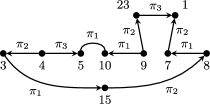
Step 2. Next, we choose how many edges	Step 3. We can choose the new vertices in
will go in each gap between components.	$[n-p-l]_{j-p-l}$ ways, and we can direct
Each gap must contain at least one edge,	and give labels to the new edges in at
and we must add a total of $j-l$ edges,	most $(2d-1)^{j-l}$ ways.
giving us ${j-l-1\choose p-1}$ choices.
In this example, we have added one edge
after $A_{1}$, three after $A_{3}$, and two after $A_{2}$.

Figure 5: Assembling an element $\beta\in\mathcal{I}_{\alpha}^{l}$ that overlaps with $\alpha$ at a given subgraph $H$.

Let $A_{1},\ldots,A_{p}$ be the components of $H$. We can assemble any element $\beta\in\mathcal{I}_{\alpha}^{l}$ that overlaps with $\alpha$ in $H$ by stringing together these components in some order, with other edges in between. Each component can appear in $\beta$ in one of two orientations. Since the vertices in $\beta$ have no fixed ordering, we can assume without loss of generality that $\beta$ begins with component $A_{1}$ with a fixed orientation. This leaves $(p-1)!2^{p-1}$ choices for the order and orientation of $A_{2},\ldots,A_{p}$ in $\beta$.

Imagine now the components laid out in a line, with gaps between them, and count the number of ways to fill the gaps. Suppose that $\beta$ is to have length $j$. Each of the $p$ gaps must contain at least one edge, and the total number of edges in all the gaps is $j-l$. Thus, the total number of possible gap sizes is the number of compositions of $j-l$ into $p$ parts, or ${j-l-1\choose p-1}$.

Now that we have chosen the number of edges to appear in each gap, we choose the edges themselves. We can do this by giving an ordered list $j-p-l$ vertices to go in the gaps, along with a label and an orientation for each of the $j-l$ edges this gives. There are $[n-p-l]_{j-p-l}$ ways to choose the vertices. We can give each new edge any orientation and label subject to the constraint that the word of the cycle we construct must be reduced. This means we have at most $2d-1$ choices for the orientation and label of each new edge, for a total of at most $(2d-1)^{j-i}$.

All together, there are at most $(p-1)!2^{p-1}{j-l-1\choose p-1}[n-p-l]_{j-p-l}(2d-1)^{j-l}$ elements of $\mathcal{I}_{j}$ that overlap with the cycle $\alpha$ at the subgraph $H$. We now calculate the number of different ways to choose a subgraph $H$ of $\alpha$ with $l$ edges and $p$ components. Suppose $\alpha$ is given as in (21). We first choose a vertex $s_{i_{0}}$. Then, we can specify which edges to include in $H$ by giving a sequence $a_{1},b_{1},\ldots,a_{p},b_{p}$ instructing us to include in $H$ the first $a_{1}$ edges after $s_{i_{0}}$, then to exclude the next $b_{1}$, then to include the next $a_{2}$, and so on. Any sequence for which $a_{i}$ and $b_{i}$ are positive integers, $a_{1}+\cdots+a_{p}=l$, and $b_{1}+\cdots+b_{p}=k-l$ gives us a valid choice of $l$ edges of $\alpha$ making up $p$ components. This counts each subgraph $H$ a total of $p$ times, since we could begin with any component of $H$. Hence, the number of subgraphs $H$ with $l$ edges and $p$ components is $(k/p){l-1\choose p-1}{k-l-1\choose p-1}$. This gives us the bound

$$\bigl{|}\mathcal{I}_{\alpha}^{l}\cap\mathcal{I}_{j}\bigr{|} \leq \sum_{p=1}^{l\wedge(j-l)}(k/p)\pmatrix{l-1\cr p-1}\pmatrix{k-l-1\cr p-1}(p-1)!$$

$$\hskip 27.0pt{}\times 2^{p-1}\pmatrix{j-l-1\cr p-1}[n-p-l]_{j-p-l}(2d-1)^{j-l}.$$

We apply the bounds

$$\pmatrix{l-1\cr p-1} \leq \frac{r^{p-1}}{(p-1)!},$$

$$\pmatrix{k-l-1\cr p-1},\pmatrix{j-l-1\cr p-1} \leq \bigl{(}er/(p-1)\bigr{)}^{p-1},$$

to get

$$\bigl{|}\mathcal{I}_{\alpha}^{l}\cap\mathcal{I}_{j}\bigr{|} \leq k(2d-1)^{j-l}[n-1-l]_{j-1-l}$$

$${}\times\Biggl{(}1+\sum_{p=2}^{i\wedge(k-i)}\frac{1}{p}\biggl{(}\frac{2e^{2}r^{3}}{(p-1)^{2}}\biggr{)}^{p-1}\frac{1}{[n-1-l]_{p-1}}\Biggr{)}.$$

Since $r\leq n^{1/10}$, the sum in the above equation is bounded by an absolute constant. Applying this bound and (25), for any $\alpha\in\mathcal{I}_{k}$ and $l\geq 1$,

$$\sum_{\beta\in\mathcal{I}_{\alpha}^{l}}\mathop{\operatorname{Cov}}(I_{\alpha},I_{\beta}) \leq \sum_{j=l+1\vphantom{\mathcal{I}_{\alpha}^{l}}}^{r}\sum_{\beta\in\mathcal{I}_{\alpha}^{l}\cap\mathcal{I}_{j}}\frac{1}{[n]_{k+j-l}}\leq\sum_{j=l+1}^{r}O\biggl{(}\frac{k(2d-1)^{j-l}}{n^{k+1}}\biggr{)}$$

$$= O\biggl{(}\frac{k(2d-1)^{r-l}}{n^{k+1}}\biggr{)}.$$

Therefore,

$$\sum_{\alpha\in\mathcal{I}}\sum_{l\geq 1}\sum_{\beta\in\mathcal{I}_{\alpha}^{l}}\mathop{\operatorname{Cov}}(I_{\alpha},I_{\beta}) = \sum_{k=1}^{r}\sum_{\alpha\in\mathcal{I}_{k}}\sum_{l=1}^{k-1}\sum_{\beta\in\mathcal{I}_{\alpha}^{l}}\mathop{\operatorname{Cov}}(I_{\alpha},I_{\beta})$$

$$\leq \sum_{k=1}^{r}\sum_{\alpha\in\mathcal{I}_{k}}\sum_{l=1}^{k-1}O\biggl{(}\frac{k(2d-1)^{r-l}}{n^{k+1}}\biggr{)}$$

$$= \sum_{k=1}^{r}\frac{[n]_{k}a(d,k)}{2k}O\biggl{(}\frac{k(2d-1)^{r-1}}{n^{k+1}}\biggr{)}$$

$$= \sum_{k=1}^{r}O\biggl{(}\frac{(2d-1)^{r+k-1}}{n}\biggr{)}$$

$$= O\biggl{(}\frac{(2d-1)^{2r-1}}{n}\biggr{)}.$$

Last, we must bound $\sum_{\alpha\in\mathcal{I}}\sum_{\beta\in\mathcal{I}_{\alpha}^{0}}\mathop{\operatorname{Cov}}(I_{\alpha},I_{\beta})$. For any word $w$, let $e^{w}_{i}$ be the number of appearances of $\pi_{i}$ and $\pi_{i}^{-1}$ in $w$. Let $\alpha$ and $\beta$ be cycles with words $w$ and $u$, respectively, and let $k=|\alpha|$ and $j=|\beta|$. Suppose that $\beta\in\mathcal{I}^{0}_{\alpha}$. Then

$$\mathop{\operatorname{Cov}}(I_{\alpha},I_{\beta}) = \prod_{i=1}^{d}\frac{1}{[n]_{e^{w}_{i}+e^{u}_{i}}}-\prod_{i=1}^{d}\frac{1}{[n]_{e^{w}_{i}}[n]_{e^{u}_{i}}}$$

$$\leq \frac{\langle e^{w},e^{u}\rangle}{n}\prod_{i=1}^{d}\frac{1}{[n]_{e^{w}_{i}+e^{u}_{i}}}\leq\frac{\langle e^{w},e^{u}\rangle}{n[n]_{k+j}}$$

by Lemma 22. For any pair of words $w\in\mathcal{W}_{k}$ and $u\in\mathcal{W}_{j}$, there are at most $[n]_{k}[n]_{j}$ pairs of cycles $\alpha,\beta\in\mathcal{I}$ with words $w$ and $u$, respectively. Enumerating over all $w\in\mathcal{W}_{k}$ and $u\in\mathcal{W}_{j}$, we count each pair of cycles $\alpha,\beta$ exactly $4kj$ times. Thus,

$$\sum_{\alpha\in\mathcal{I}_{k}}\sum_{\beta\in\mathcal{I}_{\alpha}^{0}\cap\mathcal{I}_{j}}\mathop{\operatorname{Cov}}(I_{\alpha},I_{\beta}) \leq \frac{[n]_{k}[n]_{j}}{4kjn[n]_{k+j}}\sum_{w\in\mathcal{W}_{k}}\sum_{u\in\mathcal{W}_{j}}\bigl{\langle}e^{w},e^{u}\bigr{\rangle}$$

$$\leq \frac{1+O(r^{2}/n)}{4kjn}\biggl{\langle}\sum_{w\in\mathcal{W}_{k}}e^{w},\sum_{u\in\mathcal{W}_{j}}e^{u}\biggr{\rangle}.$$

The vector $\sum_{w\in\mathcal{W}_{k}}e^{w}$ has every entry equal by symmetry, as does $\sum_{u\in\mathcal{W}_{j}}e^{u}$. Thus, each entry of $\sum_{w\in\mathcal{W}_{k}}e^{w}$ is $ka(d,k)/d$, and each entry of $\sum_{u\in\mathcal{W}_{j}}e^{u}$ is $ja(d,j)/d$. The inner product in the above equation comes to$kja(d,k)a(d,j)/d$, giving us

$$\sum_{\alpha\in\mathcal{I}_{k}}\sum_{\beta\in\mathcal{I}_{\alpha}^{0}\cap\mathcal{I}_{j}}\mathop{\operatorname{Cov}}(I_{\alpha},I_{\beta}) \leq \frac{a(d,k)a(d,j)(1+O(r^{2}/n))}{4dn}$$

$$= O\biggl{(}\frac{(2d-1)^{j+k-1}}{n}\biggr{)}.$$

Summing over all $1\leq k,j\leq r$,

$$\sum_{\alpha\in\mathcal{I}}\sum_{\beta\in\mathcal{I}^{0}_{\alpha}}\mathop{\operatorname{Cov}}(I_{\alpha},I_{\beta})=\biggl{(}\frac{(2d-1)^{2r-1}}{n}\biggr{)}.$$ (27)

We can now combine equations (2), (2), (2), and (27) with Proposition 20 to show that

$$d_{\mathrm{TV}}(\mathbf{I},\mathbf{Y})=O\biggl{(}\frac{(2d-1)^{2r-1}}{n}\biggr{)}.$$ (28)

Step 3 ((Approximation of $\mathbf{Y}$ by $\mathbf{Z}$)).

By Lemma 21 and (22),

$$d_{\mathrm{TV}}(\mathbf{Y},\mathbf{Z})\leq\sum_{\alpha\in\mathcal{I}}|\mathbf{E}Y_{\alpha}-\mathbf{E}Z_{\alpha}| \leq \sum_{k=1}^{r}\sum_{\alpha\in\mathcal{I}_{k}}\biggl{(}\frac{1}{[n]_{k}}-\frac{1}{n^{k}}\biggr{)}$$

$$= \sum_{k=1}^{r}\frac{a(d,k)}{2k}\biggl{(}1-\frac{[n]_{k}}{n^{k}}\biggr{)}.$$

Since $[n]_{k}\geq n^{k}(1-k^{2}/2n)$,

$$d_{\mathrm{TV}}(\mathbf{Y},\mathbf{Z})\leq\sum_{k=1}^{r}\frac{a(d,k)k}{4n}=O\biggl{(}\frac{r(2d-1)^{r}}{n}\biggr{)}.$$

Together with (28), this bounds the total variation distance between the laws of $\mathbf{I}$ and $\mathbf{Z}$ and proves the theorem.∎

The distributions of any functionals of $\mathbf{I}$ and $\mathbf{Z}$ satisfy the same bound in total variation distance. This gives us several results as easy corollaries, including an improvement on DJPP , Theorem 11.

Corollary 24.

(i) Let $(Z_{k},1\leq k\leq r)$ be a vector of independent Poisson random variables with $\mathbf{E}Z_{k}=a(d,k)/2k$. Let $C_{k}$ denote the number of $k$-cycles in $G_{n}$, a $2d$-regular permutation random graph on $n$ vertices. Then for some absolute constant $c$,

$$d_{\mathrm{TV}}\bigl{(}(C_{k},1\leq k\leq r),(Z_{k},1\leq k\leq r)\bigr{)}\leq\frac{c(2d-1)^{2r-1}}{n}.$$

[(ii)]

Let $(Z_{w},w\in\mathcal{W}^{\prime}_{K})$ be a vector (ii) of independent Poisson random variables with $\mathbf{E}Z_{w}=1/h(w)$. Let $C_{w}$ denote the number of cycles with word $w$ in $G_{n}$, a $2d$-regular permutation random graph on $n$ vertices. Then for some absolute constant $c$,

$$d_{\mathrm{TV}}\bigl{(}\bigl{(}C_{w},w\in\mathcal{W}^{\prime}_{K}\bigr{)},\bigl{(}Z_{w},w\in\mathcal{W}^{\prime}_{K}\bigr{)}\bigr{)}\leq\frac{c(2d-1)^{2K-1}}{n}.$$

Observe that $C_{k}=\sum_{\alpha\in\mathcal{I}_{k}}I_{\alpha}$, and that if we define $Z_{k}=\break\sum_{\alpha\in\mathcal{I}_{k}}Z_{\alpha}$, then $(Z_{k},1\leq k\leq r)$ is distributed as described. Thus (i) follows from Theorem 14.

To prove (ii), note that $C_{w}=\sum_{\alpha}I_{\alpha}$, where the sum is over all cycles in $\mathcal{I}$ with word $w$. We then define $Z_{w}$ as the analogous sum over $Z_{\alpha}$. Since the number of cycles in $\mathcal{I}$ with word $w$ is $[n]_{k}/h(w)$, we have $\mathbf{E}Z_{w}=1/h(w)$, and the total variation bound follows from Theorem 14. We can also use Theorem 14 to bound the likelihood that $G_{n}$ contains two overlapping cycles of size $r$ or less.

Corollary 25.

Let $G_{n}$ be a $2d$-regular permutation random graph on $n$ vertices. Let $E$ be the event that $G_{n}$ contains two cycles of length $r$ or less with a vertex in common. Then for some absolute constant $c^{\prime}$, for all $d\geq 2$ and $n,r\geq 1$,

$$\mathbf{P}[E]\leq\frac{c^{\prime}(2d-1)^{2r}}{n}.$$

Let $E^{\prime}$ be the event that $Z_{\alpha}=Z_{\beta}=1$ for two cycles $\alpha,\beta\in\mathcal{I}$ that have a vertex in common. By Theorem 14,

$$\mathbf{P}[E]\leq\mathbf{P}\bigl{[}E^{\prime}\bigr{]}+\frac{c(2d-1)^{2r-1}}{n}.$$

For any cycle $\alpha\in\mathcal{I}_{k}$, there are at most $k[n-1]_{j-1}a(d,j)$ cycles in $\mathcal{I}_{j}$ that share a vertex with $\alpha$. For any such cycle $\beta$, the chance that $Z_{\alpha}=1$ and $Z_{\beta}=1$ is less than $1/[n]_{k}[n]_{j}$. By a union bound,

$$\mathbf{P}\bigl{[}E^{\prime}\bigr{]} \leq \sum_{k=1}^{r}\frac{a(d,k)[n]_{k}}{2k}\sum_{j=1}^{r}\frac{k[n-1]_{j-1}a(d,j)}{[n]_{k}[n]_{j}}$$

$$\leq \sum_{k=1}^{r}\sum_{j=1}^{r}\frac{a(d,k)a(d,j)}{2n}=O\biggl{(}\frac{(2d-1)^{2r}}{n}\biggr{)}.$$

Proof of Corollary 15 When $d=1$, there is only one word of each length in $\mathcal{W}^{\prime}_{K}$, and statement (i) reduces to the well-known fact that the cycle counts of a random permutation converge to independent Poisson random variables (see AT for much more on this subject). In this case, $G(t)$ is made up of disjoint cycles for all times $t$, so that statement (ii) is trivially satisfied.

When $d\geq 2$, let $C_{w}^{(n)}$ be the number of cycles with word $w$ in $G_{n}$, as in Corollary 24(ii). The random vector $(C_{w}(t),w\in\mathcal{W}^{\prime}_{K})$ is a mixture of the random vectors $(C_{w}^{(n)},w\in\mathcal{W}^{\prime}_{K})$ over different values of $n$. That is,

$$\mathbf{P}\bigl{[}\bigl{(}C_{w}(t),w\in\mathcal{W}^{\prime}_{K}\bigr{)}\in A\bigr{]}=\sum_{n=1}^{\infty}\mathbf{P}[M_{t}=n]\mathbf{P}\bigl{[}\bigl{(}C_{w}^{(n)},w\in\mathcal{W}^{\prime}_{K}\bigr{)}\in A\bigr{]}$$

for any set $A$, recalling that $G(t)=G_{M_{t}}$. Corollary 24(ii) together with the fact that $\mathbf{P}[M_{t}>N]\to 1$ as $t\to\infty$ for any $N$ imply that $(C_{w}(t),w\in\mathcal{W}^{\prime}_{K})$ converges in law to $(Z_{w},w\in\mathcal{W}^{\prime}_{K})$, establishing statement (i). Statement (ii) follows in the same way from Corollary 25. Proof of Lemma 21 We will apply the Stein–Chen method directly. Define the operator $\mathcal{A}$ by

$$\mathcal{A}h(x)=\sum_{\alpha\in\mathcal{I}}\mathbf{E}[Z_{\alpha}]\bigl{(}h(x+e_{\alpha})-h(x)\bigr{)}+\sum_{\alpha\in\mathcal{I}}x_{\alpha}\bigl{(}h(x-e_{\alpha})-h(x)\bigr{)}$$

for any $h\dvtx\mathbb{Z}_{+}^{|\mathcal{I}|}\to\mathbb{R}$ and $x\in\mathbb{Z}_{+}^{|\mathcal{I}|}$. This is the Stein operator for the law of $\mathbf{Z}$, and $\mathbf{E}\mathcal{A}h(\mathbf{Z})=0$ for any bounded function $h$. By Proposition 10.1.2 and Lemma 10.1.3 in BHJ , for any set $A\subseteq\mathbb{Z}_{+}^{|\mathcal{I}|}$, there is a function $h$ such that

$$\mathcal{A}h(x)=1\{x\in A\}-\mathbf{P}[\mathbf{Z}\in A],$$

and this function has the property that

$$\mathop{\sup_{x\in\mathbb{Z}_{+}^{|\mathcal{I}|}}}_{\alpha\in\mathcal{I}}\bigl{|}h(x+e_{\alpha})-h(x)\bigr{|}\leq 1.$$ (29)

Thus we can bound the total variation distance between the laws of $\mathbf{Y}$ and $\mathbf{Z}$ by bounding $|\mathbf{E}\mathcal{A}h(\mathbf{Y})|$ over all such functions $h$.

We write $\mathcal{A}h(\mathbf{Y})$ as

$$\mathcal{A}h(\mathbf{Y}) = \sum_{\alpha\in\mathcal{I}}\mathbf{E}[Y_{\alpha}]\bigl{(}h(\mathbf{Y}+e_{\alpha})-h(\mathbf{Y})\bigr{)}+\sum_{\alpha\in\mathcal{I}}Y_{\alpha}\bigl{(}h(\mathbf{Y}-e_{\alpha})-h(x)\bigr{)}$$

$${}+\sum_{\alpha\in\mathcal{I}}(\mathbf{E}Z_{\alpha}-\mathbf{E}Y_{\alpha})\bigl{(}h(\mathbf{Y}+e_{\alpha})-h(\mathbf{Y})\bigr{)}.$$

The first two of these sums have expectation zero, so

$$\bigl{|}\mathbf{E}\mathcal{A}h(\mathbf{Y})\bigr{|}\leq\sum_{\alpha\in\mathcal{I}}|\mathbf{E}Z_{\alpha}-\mathbf{E}Y_{\alpha}|\mathbf{E}\bigl{|}h(\mathbf{Y}+e_{\alpha})-h(\mathbf{Y})\bigr{|}.$$

By (29), $|h(\mathbf{Y}+e_{\alpha})-h(\mathbf{Y})|\leq 1$, which proves the lemma. Proof of Lemma 22 We define a family of independent random maps $\sigma_{i}$ and $\tau_{i}$ for $1\leq i\leq d$. Choose $\sigma_{i}$ uniformly from all injective maps from $[a_{i}]$ to $[n]$, and choose $\tau_{i}$ uniformly from all injective maps from $[b_{i}]$ to $[n]$. Effectively, $\sigma_{i}$ and $\tau_{i}$ are random ordered subsets of $[n]$. We say that $\sigma_{i}$ and $\tau_{i}$ clash if their images overlap.

$$\mathbf{P}[\mbox{$\sigma_{i}$ and $\tau_{i}$ clash for some $i$}]=1-\prod_{i=1}^{d}\frac{[n]_{a_{i}+b_{i}}}{[n]_{a_{i}}[n]_{b_{i}}}.$$

For any $1\leq i\leq d$, $1\leq j\leq a_{i}$, and $1\leq k\leq b_{i}$, the probability that $\sigma_{i}(j)=\tau_{i}(k)$ is $1/n$. By a union bound,

$$\mathbf{P}[\mbox{$\sigma_{i}$ and $\tau_{i}$ clash for some $i$}]\leq\sum_{i=1}^{d}\frac{a_{i}b_{i}}{n}=\frac{\langle a,b\rangle}{n}.$$

We finish the proof by dividing both sides of this inequality by $\prod_{i=1}^{d}[n]_{a_{i}+b_{i}}$.

References

- (1) {bmisc}[auto:STB—2013/10/14—10:36:11] \bauthor\bsnmAdler, \bfnmMark\binitsM., \bauthor\bsnmNordenstam, \bfnmEric\binitsE. and \bauthor\bparticlevan \bsnmMoerbeke, \bfnmPierre\binitsP. (\byear2011). \bhowpublishedThe Dyson Brownian minor process. Preprint. Available at \arxivurlarXiv:1006.2956. \bptokimsref \endbibitem
- (2) {barticle}[mr] \bauthor\bsnmArratia, \bfnmRichard\binitsR. and \bauthor\bsnmTavaré, \bfnmSimon\binitsS. (\byear1992). \btitleThe cycle structure of random permutations. \bjournalAnn. Probab. \bvolume20 \bpages1567–1591. \bidissn=0091-1798, mr=1175278 \bptokimsref \endbibitem
- (3) {bbook}[mr] \bauthor\bsnmBarbour, \bfnmA. D.\binitsA. D., \bauthor\bsnmHolst, \bfnmLars\binitsL. and \bauthor\bsnmJanson, \bfnmSvante\binitsS. (\byear1992). \btitlePoisson Approximation. \bseriesOxford Studies in Probability \bvolume2. \bpublisherOxford Univ. Press, \blocationNew York. \bidmr=1163825 \bptokimsref \endbibitem
- (4) {bmisc}[auto:STB—2013/10/14—10:36:11] \bauthor\bsnmBen Arous, \bfnmGérard\binitsG. and \bauthor\bsnmDang, \bfnmKim\binitsK. (\byear2011). \bhowpublishedOn fluctuations of eigenvalues of random permutation matrices. Preprint. Available at \arxivurlarXiv:1106.2108. \bptokimsref \endbibitem
- (5) {bbook}[mr] \bauthor\bsnmBillingsley, \bfnmPatrick\binitsP. (\byear1999). \btitleConvergence of Probability Measures, \bedition2nd ed. \bpublisherWiley, \blocationNew York. \biddoi=10.1002/9780470316962, mr=1700749 \bptokimsref \endbibitem
- (6) {bmisc}[auto:STB—2013/10/14—10:36:11] \bauthor\bsnmBorodin, \bfnmAlexei\binitsA. (\byear2010). \bhowpublishedCLT for spectra of submatrices of Wigner random matrices. Preprint. Available at \arxivurlarXiv:1010.0898. \bptokimsref \endbibitem
- (7) {bmisc}[auto:STB—2013/10/14—10:36:11] \bauthor\bsnmBorodin, \bfnmAlexei\binitsA. (\byear2010). \bhowpublishedCLT for spectra of submatrices of Wigner random matrices II. Stochastic evolution. Preprint. Available at \arxivurlarXiv:1011.3544. \bptokimsref \endbibitem
- (8) {bmisc}[mr] \bauthor\bsnmBorodin, \bfnmAlexei\binitsA. and \bauthor\bsnmFerrari, \bfnmPatrik L.\binitsP. L. (\byear2008). \bhowpublishedAnisotropic growth of random surfaces in dimensions. Preprint. Available at \arxivurlarXiv:0804.3035. \bptokimsref \endbibitem
- (9) {barticle}[auto:STB—2013/10/14—10:36:11] \bauthor\bsnmBourgade, \bfnmPaul\binitsP., \bauthor\bsnmNajnudel, \bfnmJoseph\binitsJ. and \bauthor\bsnmNikeghbali, \bfnmAshkan\binitsA. (\byear2013). \btitleA unitary extension of virtual permutations. \bjournalInt. Math. Res. Not. IMRN \bvolume2013 \bpages4101–4134. \bidmr=3106884 \bptokimsref \endbibitem
- (10) {barticle}[mr] \bauthor\bsnmCarmona, \bfnmPhilippe\binitsP., \bauthor\bsnmPetit, \bfnmFrédérique\binitsF. and \bauthor\bsnmYor, \bfnmMarc\binitsM. (\byear1998). \btitleBeta-gamma random variables and intertwining relations between certain Markov processes. \bjournalRev. Mat. Iberoam. \bvolume14 \bpages311–367. \biddoi=10.4171/RMI/241, issn=0213-2230, mr=1654531 \bptokimsref \endbibitem
- (11) {barticle}[mr] \bauthor\bsnmDiaconis, \bfnmPersi\binitsP. and \bauthor\bsnmFill, \bfnmJames Allen\binitsJ. A. (\byear1990). \btitleStrong stationary times via a new form of duality. \bjournalAnn. Probab. \bvolume18 \bpages1483–1522. \bidissn=0091-1798, mr=1071805 \bptokimsref \endbibitem
- (12) {barticle}[mr] \bauthor\bsnmDumitriu, \bfnmIoana\binitsI., \bauthor\bsnmJohnson, \bfnmTobias\binitsT., \bauthor\bsnmPal, \bfnmSoumik\binitsS. and \bauthor\bsnmPaquette, \bfnmElliot\binitsE. (\byear2013). \btitleFunctional limit theorems for random regular graphs. \bjournalProbab. Theory Related Fields \bvolume156 \bpages921–975. \biddoi=10.1007/s00440-012-0447-y, issn=0178-8051, mr=3078290 \bptnotecheck year\bptokimsref \endbibitem
- (13) {barticle}[mr] \bauthor\bsnmDumitriu, \bfnmIoana\binitsI. and \bauthor\bsnmPal, \bfnmSoumik\binitsS. (\byear2012). \btitleSparse regular random graphs: Spectral density and eigenvectors. \bjournalAnn. Probab. \bvolume40 \bpages2197–2235. \biddoi=10.1214/11-AOP673, issn=0091-1798, mr=3025715 \bptokimsref \endbibitem
- (14) {barticle}[mr] \bauthor\bsnmElon, \bfnmYehonatan\binitsY. (\byear2008). \btitleEigenvectors of the discrete Laplacian on regular graphs—A statistical approach. \bjournalJ. Phys. A \bvolume41 \bpages435203, 17. \biddoi=10.1088/1751-8113/41/43/435203, issn=1751-8113, mr=2453165 \bptokimsref \endbibitem
- (15) {bmisc}[auto:STB—2013/10/14—10:36:11] \bauthor\bsnmElon, \bfnmYehonatan\binitsY. (\byear2010). \bhowpublishedGaussian waves on the regular tree. Preprint. Available at \arxivurlarXiv:0907.5065. \bptokimsref \endbibitem
- (16) {barticle}[mr] \bauthor\bsnmElon, \bfnmYehonatan\binitsY. and \bauthor\bsnmSmilansky, \bfnmUzy\binitsU. (\byear2010). \btitlePercolating level sets of the adjacency eigenvectors of -regular graphs. \bjournalJ. Phys. A \bvolume43 \bpages455209, 13. \biddoi=10.1088/1751-8113/43/45/455209, issn=1751-8113, mr=2733852 \bptokimsref \endbibitem
- (17) {bbook}[mr] \bauthor\bsnmEthier, \bfnmStewart N.\binitsS. N. and \bauthor\bsnmKurtz, \bfnmThomas G.\binitsT. G. (\byear1986). \btitleMarkov Processes: Characterization and Convergence. \bpublisherWiley, \blocationNew York. \biddoi=10.1002/9780470316658, mr=0838085 \bptokimsref \endbibitem
- (18) {barticle}[mr] \bauthor\bsnmFerrari, \bfnmPatrik L.\binitsP. L. (\byear2010). \btitleFrom interacting particle systems to random matrices. \bjournalJ. Stat. Mech. Theory Exp. \bvolume10 \bpagesP10016, 15. \bidissn=1742-5468, mr=2800495 \bptokimsref \endbibitem
- (19) {barticle}[mr] \bauthor\bsnmFerrari, \bfnmPatrik L.\binitsP. L. and \bauthor\bsnmFrings, \bfnmRené\binitsR. (\byear2010). \btitleOn the partial connection between random matrices and interacting particle systems. \bjournalJ. Stat. Phys. \bvolume141 \bpages613–637. \biddoi=10.1007/s10955-010-0070-1, issn=0022-4715, mr=2733398 \bptokimsref \endbibitem
- (20) {bincollection}[mr] \bauthor\bsnmJakobson, \bfnmDmitry\binitsD., \bauthor\bsnmMiller, \bfnmStephen D.\binitsS. D., \bauthor\bsnmRivin, \bfnmIgor\binitsI. and \bauthor\bsnmRudnick, \bfnmZeév\binitsZ. (\byear1999). \btitleEigenvalue spacings for regular graphs. In \bbooktitleEmerging Applications of Number Theory (Minneapolis, MN, 1996). \bseriesIMA Vol. Math. Appl. \bvolume109 \bpages317–327. \bpublisherSpringer, \blocationNew York. \biddoi=10.1007/978-1-4612-1544-8_12, mr=1691538 \bptokimsref \endbibitem
- (21) {barticle}[mr] \bauthor\bsnmJohansson, \bfnmKurt\binitsK. and \bauthor\bsnmNordenstam, \bfnmEric\binitsE. (\byear2006). \btitleEigenvalues of GUE minors. \bjournalElectron. J. Probab. \bvolume11 \bpages1342–1371. \biddoi=10.1214/EJP.v11-370, issn=1083-6489, mr=2268547 \bptokimsref \endbibitem
- (22) {bmisc}[auto] \bauthor\bsnmJohnson, \bfnmT.\binitsT. (\byear2014). \bhowpublishedEigenvalue fluctuations for random regular graphs. Ph.D. thesis, Univ. Washington. \bptokimsref \endbibitem
- (23) {barticle}[mr] \bauthor\bsnmKerov, \bfnmSergei\binitsS., \bauthor\bsnmOlshanski, \bfnmGrigori\binitsG. and \bauthor\bsnmVershik, \bfnmAnatoly\binitsA. (\byear2004). \btitleHarmonic analysis on the infinite symmetric group. \bjournalInvent. Math. \bvolume158 \bpages551–642. \biddoi=10.1007/s00222-004-0381-4, issn=0020-9910, mr=2104794 \bptokimsref \endbibitem
- (24) {barticle}[mr] \bauthor\bsnmLinial, \bfnmNati\binitsN. and \bauthor\bsnmPuder, \bfnmDoron\binitsD. (\byear2010). \btitleWord maps and spectra of random graph lifts. \bjournalRandom Structures Algorithms \bvolume37 \bpages100–135. \biddoi=10.1002/rsa.20304, issn=1042-9832, mr=2674623 \bptokimsref \endbibitem
- (25) {barticle}[mr] \bauthor\bsnmMiller, \bfnmSteven J.\binitsS. J. and \bauthor\bsnmNovikoff, \bfnmTim\binitsT. (\byear2008). \btitleThe distribution of the largest nontrivial eigenvalues in families of random regular graphs. \bjournalExperiment. Math. \bvolume17 \bpages231–244. \bidissn=1058-6458, mr=2433888 \bptokimsref \endbibitem
- (26) {barticle}[mr] \bauthor\bsnmOren, \bfnmIdan\binitsI., \bauthor\bsnmGodel, \bfnmAmit\binitsA. and \bauthor\bsnmSmilansky, \bfnmUzy\binitsU. (\byear2009). \btitleTrace formulae and spectral statistics for discrete Laplacians on regular graphs. I. \bjournalJ. Phys. A \bvolume42 \bpages415101, 20. \biddoi=10.1088/1751-8113/42/41/415101, issn=1751-8113, mr=2545624 \bptokimsref \endbibitem
- (27) {barticle}[mr] \bauthor\bsnmOren, \bfnmIdan\binitsI. and \bauthor\bsnmSmilansky, \bfnmUzy\binitsU. (\byear2010). \btitleTrace formulas and spectral statistics for discrete Laplacians on regular graphs (II). \bjournalJ. Phys. A \bvolume43 \bpages225205, 13. \biddoi=10.1088/1751-8113/43/22/225205, issn=1751-8113, mr=2647344 \bptokimsref \endbibitem
- (28) {bbook}[mr] \bauthor\bsnmPitman, \bfnmJ.\binitsJ. (\byear2006). \btitleCombinatorial Stochastic Processes. \bseriesLecture Notes in Math. \bvolume1875. \bpublisherSpringer, \blocationBerlin. \bidmr=2245368 \bptokimsref \endbibitem
- (29) {barticle}[mr] \bauthor\bsnmSheffield, \bfnmScott\binitsS. (\byear2007). \btitleGaussian free fields for mathematicians. \bjournalProbab. Theory Related Fields \bvolume139 \bpages521–541. \biddoi=10.1007/s00440-006-0050-1, issn=0178-8051, mr=2322706 \bptokimsref \endbibitem
- (30) {barticle}[auto:STB—2013/10/14—10:36:11] \bauthor\bsnmSmilansky, \bfnmUzy\binitsU. (\byear2010). \btitleDiscrete graphs—A paradigm model for quantum chaos. \bjournalSéminaire Poincaré \bvolumeXIV \bpages89–114. \bnoteAvailable at http://www.bourbaphy.fr/smilansky.pdf. \bptokimsref \endbibitem
- (31) {barticle}[mr] \bauthor\bsnmSpohn, \bfnmH.\binitsH. (\byear1998). \btitleDyson’s model of interacting Brownian motions at arbitrary coupling strength. \bjournalMarkov Process. Related Fields \bvolume4 \bpages649–661. \bidissn=1024-2953, mr=1677063 \bptokimsref \endbibitem
- (32) {barticle}[mr] \bauthor\bsnmTran, \bfnmLinh V.\binitsL. V., \bauthor\bsnmVu, \bfnmVan H.\binitsV. H. and \bauthor\bsnmWang, \bfnmKe\binitsK. (\byear2013). \btitleSparse random graphs: Eigenvalues and eigenvectors. \bjournalRandom Structures Algorithms \bvolume42 \bpages110–134. \biddoi=10.1002/rsa.20406, issn=1042-9832, mr=2999215 \bptokimsref \endbibitem
- (33) {barticle}[mr] \bauthor\bsnmWieand, \bfnmKelly\binitsK. (\byear2000). \btitleEigenvalue distributions of random permutation matrices. \bjournalAnn. Probab. \bvolume28 \bpages1563–1587. \biddoi=10.1214/aop/1019160498, issn=0091-1798, mr=1813834 \bptokimsref \endbibitem
- (34) {bincollection}[mr] \bauthor\bsnmWormald, \bfnmN. C.\binitsN. C. (\byear1999). \btitleModels of random regular graphs. In \bbooktitleSurveys in Combinatorics, 1999 (Canterbury). \bseriesLondon Mathematical Society Lecture Note Series \bvolume267 \bpages239–298. \bpublisherCambridge Univ. Press, \blocationCambridge. \bidmr=1725006 \bptokimsref \endbibitem