Accuracy of the Tracy–Widom limits for the extreme eigenvalues in white Wishart matrices

Abstract

The distributions of the largest and the smallest eigenvalues of a $p$-variate sample covariance matrix $S$ are of great importance in statistics. Focusing on the null case where $nS$ follows the standard Wishart distribution $W_{p}(I,n)$, we study the accuracy of their scaling limits under the setting: $n/p\rightarrow\gamma\in(0,\infty)$ as $n\rightarrow\infty$. The limits here are the orthogonal Tracy–Widom law and its reflection about the origin.

With carefully chosen rescaling constants, the approximation to the rescaled largest eigenvalue distribution by the limit attains accuracy of order ${\mathrm{O}({\min(n,p)^{-2/3}})}$. If $\gamma>1$, the same order of accuracy is obtained for the smallest eigenvalue after incorporating an additional log transform. Numerical results show that the relative error of approximation at conventional significance levels is reduced by over $50\%$ in rectangular and over $75\%$ in ‘thin’ data matrix settings, even with $\min(n,p)$ as small as $2$.

1 Introduction

Understanding the behavior of the extreme eigenvalues of a sample covariance matrix $S$ is important in a large number of multivariate statistical problems. As an example, consider one of the most common inference problems: testing the null hypothesis that the population covariance is identity. Roy’s union intersection principle [29] suggests that we reject the null hypothesis for large values of the largest eigenvalue of $S$ (or for small values of the smallest eigenvalue). Naturally, the next question is: How should the $p$-value be calculated?

To address this issue, and many others, it is necessary to examine the null distributions of the extreme sample eigenvalues. In this paper, we restrict ourselves to the Gaussian framework. In particular, let $X$ be an $n\times p$ data matrix whose row vectors are i.i.d. samples from the $N_{p}(0,I)$ distribution. The $p\times p$ matrix $A=X^{\prime}X$ then follows a standard Wishart distribution: $A\sim W_{p}(I,n)$, and is called a (real) white Wishart matrix. The ordered eigenvalues of $A$ are denoted by $\lambda_{1}\geq\cdots\geq\lambda_{p}$. Our interest lies in $\lambda_{1}$ and $\lambda_{p}$, as $A=nS$.

The exact evaluation of the marginal distributions of these eigenvalues is difficult, even in the null case considered here. See, for example, Muirhead [24], Section 9.7. An alternative approach is to approximate them by their asymptotic limits. For the problem we are concerned with, Anderson [2], Chapter 13, summarized the classical results under the conventional asymptotic regime: $p$ holds fixed and $n$ tends to infinity.

However, for a wide range of modern data sets (microarray data, stock prices, weather forecasting, etc.), the number of features $p$ is very large while the number of observations $n$ is much smaller than or just comparable to $p$. For these situations, the classical asymptotics is not always appropriate and different asymptotic theories are needed. Borrowing tools from random matrix theory, especially those established by Tracy and Widom [32, 33, 34], Johnstone [15] showed that under the asymptotic regime

$$p\rightarrow\infty,\qquad n=n(p)\rightarrow\infty\quad\mbox{and}\quad n/p\rightarrow\gamma\in(0,\infty),$$ (1)

the largest eigenvalue $\lambda_{1}$ in $A$ has the weak limit

$$\frac{\lambda_{1}-\mu_{p}}{\sigma_{p}}\stackrel{{\scriptstyle\mathcal{D}}}{{\longrightarrow}}F_{1},$$ (2)

where the centering and scaling constants are defined as

$$\mu_{p}=\bigl{(}\sqrt{n-1}+\sqrt{p}\bigr{)}^{2},\qquad\sigma_{p}=\bigl{(}\sqrt{n-1}+\sqrt{p}\bigr{)}\biggl{(}\frac{1}{\sqrt{n-1}}+\frac{1}{\sqrt{p}}\biggr{)}^{1/3}.$$ (3)

Here $F_{1}$ denotes the orthogonal-Tracy–Widom law [33], the scaling limit of the largest eigenvalue in real Gaussian Wigner matrices. Slightly prior to [15], as a by-product of his analysis on the random growth model, Johansson [14] proved that the scaling limit for the largest eigenvalue in the complex white Wishart matrix is the unitary Tracy–Widom law $F_{2}$. Recently, El Karoui [9] extended the asymptotic regime (1) to include the cases where $n/p\rightarrow 0$ or $\infty$. For the smallest eigenvalue, when $\gamma>1$, Baker et al. [3] showed that the reflection of $F_{2}$ about the origin is the scaling limit for complex Wishart matrices, and Paul [28] gave the Tracy–Widom limits in the case where $n/p\rightarrow\infty$ for both complex and real Wishart matrices.

Although this type of asymptotic result has emerged only recently in the statistics literature, it has already found its relevance to applications with modern data. For instance, based on (2), Patterson et al. [27] developed a formal procedure for testing the presence of population heterogeneity with SNP (single nucleotide polymorphism) data.

From a statistical point of view, to inform the use of any asymptotic result in practice, we need to understand how closely the asymptotic limit approximates the finite sample distributions. In the motivating example, this dictates the accuracy of the nominal $p$-value.

In this paper, we first establish a rate of convergence result for the Tracy–Widom approximation to the distribution of the rescaled largest eigenvalue, but with more carefully chosen constants than (3). Set $a\wedge b=\min(a,b)$ and $m_{\pm}=m\pm\frac{1}{2}$. We show that modifying the centering and scaling constants to

$$\mu_{n,p}=\bigl{(}\sqrt{n_{-}}+\sqrt{p_{-}}\bigr{)}^{2},\qquad\sigma_{n,p}=\bigl{(}\sqrt{n_{-}}+\sqrt{p_{-}}\bigr{)}\biggl{(}\frac{1}{\sqrt{n_{-}}}+\frac{1}{\sqrt{p_{-}}}\biggr{)}^{1/3}$$ (4)

results in better approximation. The difference between the distribution of $(\lambda_{1}-\mu_{n,p})/\sigma_{n,p}$ and $F_{1}$ reduces to the ‘second order’, being ${\mathrm{O}({(n\wedge p)^{-2/3}})}$ rather than ${\mathrm{O}({(n\wedge p)^{-1/3}})}$, that would apply by using (3). See Theorem 1. Numerical work in Section 2.2.1 suggests that the improvement is substantial.

Further assuming $\gamma>1$ in (1), we find that, with a log transform, the scaling limit of $\log\lambda_{p}$ is the reflected Tracy–Widom law $G_{1}$ (defined by $G_{1}(s)=1-F_{1}(-s)$) [28]. Moreover, with appropriate rescaling constants, the accuracy of the limit also reaches the second order: ${\mathrm{O}({p^{-2/3}})}$. See Theorem 2 and Section 2.2.2.

In the literature, El Karoui [10] established a parallel result for Johansson’s theorem for the largest eigenvalue on the complex domain and Choup [6] studied the same problem via an Edgeworth expansion approach. Recently, Johnstone [16] obtained both scaling limit and convergence rates for the extreme eigenvalues of an $F$-matrix, on both complex and real domains. As is usual in the Random Matrix Theory literature, results on the real domain are founded in part on those for complex data but require significant additional constructs and arguments. This is explained for our setting in Sections 3 and 4.

The rest of the paper is organized as follows. In Section 2, we present theorems for both the largest and the smallest eigenvalues, together with supporting numerical results, related statistical settings, a real data example and a brief discussion. Section 3 proves the theorem on the largest eigenvalue and Section 4 sketches the proof of the one on the smallest eigenvalue. Finally, Section 5 establishes necessary Laguerre polynomial asymptotics, which is first used without proof in Section 3. Technical details are collected in the Appendix.

2 Main results and their applications

In this section, we first state two main theorems of this paper, which are concerned with the convergence rates of the largest and the smallest eigenvalues in finite Wishart matrices to their Tracy–Widom limits. The theorems are then complemented and further justified by a series of numerical experiments, in which the Tracy–Widom approximation is reasonably good even when $n$ and/or $p$ are as small as $2$. After that, we review several related statistical settings and consider a real data example. Finally, we end the section with a brief discussion.

2.1 Main theorems

We begin with the largest eigenvalue, for which we have the following rate of convergence result.

Theorem 1

Let $A\sim W_{p}(I,n)$ with $n\neq p$ and $\lambda_{1}$ its largest eigenvalue. Define $(\mu_{n,p},\sigma_{n,p})$ as in (4). Under condition (1), for any given $s_{0}$, there exists an integer $N_{0}(s_{0},\gamma)$, such that when $n\wedge p\geq N_{0}(s_{0},\gamma)$ and is even, for all $s\geq s_{0}$,

$$|P\{\lambda_{1}\leq\mu_{n,p}+\sigma_{n,p}s\}-F_{1}(s)|\leq C(s_{0})(n\wedge p)^{-2/3}\exp(-s/2),$$

where $C(\cdot)$ is continuous and non-increasing.

We also obtain an analogous result for the smallest eigenvalue. Refine condition (1) to

$$p\rightarrow\infty,\qquad p+1\leq n=n(p)\rightarrow\infty\quad\mbox{and}\quad n/p\rightarrow\gamma\in(1,\infty).$$ (5)

Define $\mu_{n,p}^{-}=(\sqrt{n_{-}}-\sqrt{p_{-}})^{2}$, $\sigma_{n,p}^{-}=(\sqrt{n_{-}}-\sqrt{p_{-}})({1}/{\sqrt{p_{-}}}-{1}/{\sqrt{n_{-}}})^{1/3}$, and let

$$\tau^{-}_{n,p}=\frac{\sigma^{-}_{n,p}}{\mu^{-}_{n,p}},\qquad\nu^{-}_{n,p}=\log(\mu^{-}_{n,p})+\frac{1}{8}(\tau^{-}_{n,p})^{2}.$$ (6)

Then we have the following theorem.

Theorem 2

Let $A\sim W_{p}(I,n)$ with $n-1\geq p$ and $\lambda_{p}$ as its smallest eigenvalue. Define $(\nu^{-}_{n,p},\tau^{-}_{n,p})$ as in (6). Under condition (5), we have

$$\frac{\log\lambda_{p}-\nu^{-}_{n,p}}{\tau^{-}_{n,p}}\stackrel{{\scriptstyle\mathcal{D}}}{{\longrightarrow}}G_{1}$$

with $G_{1}(s)=1-F_{1}(-s),$ the reflected Tracy–Widom law.

In addition, for any given $s_{0}$, there exists an integer $N_{0}(s_{0},\gamma)$, such that when $p\geq N_{0}(s_{0},\gamma)$ and is even, for all $s\geq s_{0}$,

$$|P\{\log\lambda_{p}\leq\nu^{-}_{n,p}-\tau^{-}_{n,p}s\}-G_{1}(-s)|\leq C(s_{0})p^{-2/3}\exp(-s/2),$$

where $C(\cdot)$ is continuous and non-increasing.

Table 1: Simulations for finite $n\times p$ vs. Tracy–Widom limit: the largest eigenvalue. For each $(n,p)$ combination, we show in the first row empirical cumulative probabilities for $\lambda_{1}$, rescaled by (4), and the second row, with parentheses, rescaled by (3), both computed from $R=40\,000$ repeated draws from $W_{p}(n,I)$ using the method in [7]. Conventional significance levels are highlighted in bold font and the last row gives approximate standard errors based on binomial sampling. $F_{1}$ was computed by the method in [8] with percentiles obtained via inverse interpolation

Percentiles	$-3.8954$	$-3.1804$	$-2.7824$	$-1.9104$	$-1.2686$	$-0.5923$	$0.4501$	$0.9793$	$2.0234$
TW	$0.01$	$0.05$	$0.10$	$0.30$	$0.50$	$0.70$	0.90	0.95	0.99
$2\times 2$	$0.000$	$0.000$	$0.000$	$0.034$	$0.379$	$0.690$	0.908	0.953	0.988
	$(0.000)$	$(0.000)$	$(0.000)$	$(0.015)$	$(0.345)$	$(0.669)$	$(0.902)$	$(0.950)$	(0.987)
$5\times 5$	$0.000$	$0.002$	$0.021$	$0.218$	$0.465$	$0.702$	0.908	0.954	0.989
	$(0.000)$	$(0.002)$	$(0.020)$	$(0.213)$	$(0.460)$	$(0.698)$	$(0.907)$	$(0.953)$	(0.989)
$25\times 25$	$0.003$	$0.031$	$0.075$	$0.280$	$0.492$	$0.700$	0.902	0.951	0.990
	$(0.003)$	$(0.030)$	$(0.075)$	$(0.280)$	$(0.491)$	$(0.699)$	$(0.902)$	$(0.951)$	(0.990)
$100\times 100$	$0.007$	$0.041$	$0.091$	$0.294$	$0.501$	$0.704$	0.902	0.951	0.990
	$(0.007)$	$(0.041)$	$(0.091)$	$(0.294)$	$(0.501)$	$(0.704)$	$(0.902)$	$(0.951)$	(0.990)
$8\times 2$	$0.000$	$0.001$	$0.012$	$0.196$	$0.456$	$0.702$	0.909	0.955	0.990
	$(0.000)$	$(0.004)$	$(0.031)$	$(0.270)$	$(0.532)$	$(0.754)$	$(0.928)$	$(0.964)$	(0.992)
$20\times 5$	$0.001$	$0.018$	$0.054$	$0.259$	$0.483$	$0.704$	0.906	0.954	0.990
	$(0.002)$	$(0.028)$	$(0.073)$	$(0.303)$	$(0.531)$	$(0.737)$	$(0.921)$	$(0.962)$	(0.992)
$100\times 25$	$0.006$	$0.040$	$0.088$	$0.292$	$0.498$	$0.701$	0.901	0.950	0.989
	$(0.008)$	$(0.047)$	$(0.100)$	$(0.314)$	$(0.523)$	$(0.721)$	$(0.910)$	$(0.955)$	(0.991)
$400\times 100$	$0.009$	$0.048$	$0.096$	$0.299$	$0.502$	$0.702$	0.902	0.951	0.990
	$(0.010)$	$(0.053)$	$(0.104)$	$(0.312)$	$(0.516)$	$(0.714)$	$(0.908)$	$(0.954)$	(0.991)
$500\times 5$	$0.010$	$0.049$	$0.098$	$0.296$	$0.502$	$0.705$	0.906	0.955	0.990
	$(0.020)$	$(0.083)$	$(0.150)$	$(0.385)$	$(0.589)$	$(0.772)$	$(0.933)$	$(0.969)$	(0.994)
$1000\times 10$	$0.010$	$0.051$	$0.101$	$0.300$	$0.504$	$0.707$	0.902	0.952	0.991
	$(0.017)$	$(0.077)$	$(0.138)$	$(0.366)$	$(0.571)$	$(0.757)$	$(0.923)$	$(0.963)$	(0.994)
$5000\times 5$	$0.012$	$0.056$	$0.107$	$0.307$	$0.509$	$0.707$	0.905	0.953	0.992
	$(0.027)$	$(0.097)$	$(0.169)$	$(0.402)$	$(0.602)$	$(0.779)$	$(0.933)$	$(0.969)$	(0.994)
$10\,000\times 10$	$0.012$	$0.055$	$0.108$	$0.308$	$0.504$	$0.706$	0.905	0.954	0.991
	$(0.021)$	$(0.084)$	$(0.150)$	$(0.378)$	$(0.580)$	$(0.763)$	$(0.929)$	$(0.967)$	(0.994)
$2\times\mathrm{SE}$	$0.001$	$0.002$	$0.003$	$0.005$	$0.005$	$0.005$	$0.003$	$0.002$	0.001

While we only prove rigorous bounds for even $p$, numerical experiments show that the approximation works just as well in the odd case, and for the largest eigenvalue, also in the square case. See Tables 1 and 2.

2.2 Numerical performance

An important motivation for the current study is to promote practical use of the Tracy–Widom approximation. To this end, we conduct here a set of experiments to investigate its numerical quality.

2.2.1 The largest eigenvalue

Distributional approximation

We first computed the empirical cumulative probabilities of $\lambda_{1}$ (after rescaling), at a collection of $F_{1}$ percentiles, using $R=40\,000$ replications. This is done for three different categories of ($n,p$) combinations: (1) the square case, where $n=p=2$, $5$, $25$ and $100$; (2) the rectangular case, where $p=2$, $5$, $25$ and $100$ and $n/p$ is fixed at 4:1; (3) the ‘thin’ case, where $p=5$ and $10$ but $n/p$ could be as high as 100:1 and 1000:1. In some sense, this category could also be thought of as in the situation where $n/p\rightarrow\infty$ as discussed in [9]. For comparison purpose, we rescaled $\lambda_{1}$ using both the new constants (4) and the old ones (3). The results are summarized in Table 1.

Table 2: Simulations for finite $n\times p$ vs. Tracy–Widom limit: the smallest eigenvalue. For each $(n,p)$ combination, empirical cumulative probabilities are computed for $(\log\lambda_{p}-\nu^{-}_{n,p})/\tau^{-}_{n,p}$ using $R=40\,000$ draws from $W_{p}(I,n)$. Methods for sampling, computing $F_{1}$ and obtaining percentiles are the same as in Table 1. Conventional significance levels are highlighted in bold font and the last line gives approximate standard errors based on binomial sampling

Percentiles	3.8954	3.1804	2.7824	1.9104	1.2686	0.5923	$-$0.4501	$-$0.9793	$-$2.0234
RTW	$0.99$	$0.95$	$0.90$	$0.70$	$0.50$	$0.30$	0.10	0.05	0.01
$4\times 2$	$1.000$	$1.000$	$0.998$	$0.893$	$0.625$	$0.326$	0.087	0.041	0.009
$10\times 5$	$0.999$	$0.995$	$0.976$	$0.798$	$0.555$	$0.310$	0.095	0.047	0.011
$50\times 25$	$0.997$	$0.973$	$0.931$	$0.728$	$0.515$	$0.302$	0.097	0.048	0.010
$200\times 100$	$0.993$	$0.960$	$0.913$	$0.713$	$0.509$	$0.306$	0.103	0.050	0.010
$8\times 2$	$1.000$	$0.992$	$0.969$	$0.792$	$0.554$	$0.314$	0.095	0.046	0.010
$20\times 5$	$0.999$	$0.977$	$0.939$	$0.740$	$0.522$	$0.301$	0.096	0.047	0.009
$100\times 25$	$0.993$	$0.960$	$0.915$	$0.713$	$0.505$	$0.298$	0.098	0.048	0.009
$400\times 100$	$0.992$	$0.954$	$0.904$	$0.701$	$0.500$	$0.298$	0.100	0.049	0.010
$2\times\mathrm{SE}$	$0.001$	$0.002$	$0.003$	$0.005$	$0.005$	$0.005$	0.003	0.002	0.001

Numerical accuracy with the new constants could be viewed from two aspects. First, for the conventional significance levels of $10\%$, $5\%$ and $1\%$ that correspond to right tails of the distributions, the approximation looks good even when $p$ is as small as $2$! In addition, it improves as $p$ becomes larger and starts to match the finite distributions almost exactly when $p$ is no greater than $25$. See the last three columns of Table 1. Second, when $p$ is large, for instance, in the $100\times 100$ and $400\times 100$ cases, $F_{1}$ provides reasonable approximation over the whole range of interest.

As regards the comparison between different rescaling constants, neither choice seems superior to the other in the square cases (see the first block of Table 1). However, when the ratio $n/p$ is changed to 4:1 or higher (see the second and the third blocks), the improvement by using new constants (4) is self-evident.

As a remark, better performance on right tails and improvement by using the new constants, as reflected in this simulation study, agree well with the mathematical statement in Theorem 1.

Approximate percentiles

We can also use $F_{1}$ to calculate approximate percentiles for the finite distributions, whose accuracy can be measured by the relative error $r_{\alpha}=\theta^{TW}_{\alpha}/\theta_{\alpha}-1$. Here, $\theta_{\alpha}$ is the exact $100\alpha$th percentile of the rescaled largest eigenvalue in the finite $n\times p$ model and $\theta^{TW}_{\alpha}$ is its counterpart from $F_{1}$.

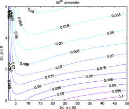
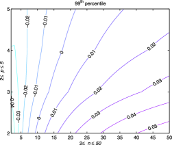
(a)	(b)

Figure 1: Plots of relative errors $r_{\alpha}$ for approximate percentiles using $F_{1}$: (a) $95$th percentile; (b) $99$th percentile. Exact finite $n\times p$ distributions are computed in MATLAB using Koev’s implementation [20] and $F_{1}$ is computed using the method in [8]. The percentiles are obtained from inverse interpolation.

In Figure 1, we plot $r_{\alpha}$ for $\alpha=0.95$ and $0.99$, with $p$ ranging from $2$ to $5$ and $n$ from $2$ to $50$. Although $n\wedge p$ is no greater than $5$, the approximation is reasonably satisfactory. For the $95$th percentile, $|r_{0.95}|$ ranges from $5\%$ to $10\%$ for most cases and slightly exceeds $10\%$ only when $p=2$ and the $n/p$ ratio is high. The approximation works even better for the $99$th percentile, with $|r_{0.99}|\leq 5\%$ for most cases. Due to computational limitation [20], we could not obtain exact percentiles when $n$ and $p$ are large. We expect the approximate percentiles to become more accurate as a consequence of better distributional approximation.

2.2.2 The smallest eigenvalue

For the smallest eigenvalue, we perform a simulation study to investigate the distributional approximation. We chose two $n/p$ ratios: 2:1 and 4:1, both with $p=2$, $5$, $25$ and $100$. For each $(n,p)$ combination, we used $R=40\,000$ replications. The simulation results shown in Table 2 demonstrate similar performance as in the case of the largest eigenvalue and agree well with Theorem 2.

2.3 Related statistical settings

Here, we review several settings in multivariate statistics to which our results are applicable. Throughout the subsection, we only use the largest eigenvalue to illustrate.

Principal component analysis

Suppose that $X=[{X}_{1},\ldots,{X}_{n}]^{\prime}$ is a Gaussian data matrix. Write the sample covariance matrix ${S}=(n-1)^{-1}{X}^{\prime}{H}{X},$ where ${H}={I}-n^{-1}\mathbf{1}\mathbf{1}^{\prime}$ is the centering matrix and principal component analysis (PCA) looks for a sequence of standardized vectors ${a}_{1},\ldots,{a}_{p}$ in $\mathbb{R}^{p}$, such that ${a}_{i}$ successively solves the following optimization problem:

$$\max\{{a}^{\prime}{S}{a}\mathchoice{\nobreak\,\colon}{\nobreak\,\colon}{\nobreak\,\colon\;}{\nobreak\,\colon\;}{a}^{\prime}{a}_{j}=0,j\leq i\},$$

where ${a}_{0}$ is the zero vector. Then, successive sample eigenvalues $\hat{\ell}_{1}\geq\cdots\geq\hat{\ell}_{p}$ satisfy $\hat{\ell}_{i}={a}^{\prime}_{i}{S}{a}_{i}$.

One basic question in PCA application is testing the hypothesis of isotropic variation, that is, the population covariance matrix $\Sigma=\tau^{2}I$. For simplicity, assume that $\tau^{2}=1$ (otherwise we divide $S$ by $\tau^{2}$). Then $(n-1){S}\sim W_{p}({I},n-1)$. The largest eigenvalue $\hat{\ell}_{1}$ of ${S}$ is a natural test statistic under the union intersection principle. Our result applies to $(n-1)\hat{\ell}_{1}$. If $\tau^{2}$ is unknown, we could estimate it by $\operatorname{tr}{S}/p$. See [25].

Testing that a covariance matrix equals a specified matrix

Suppose that $X=[X_{1},\ldots,X_{n}]^{\prime}$ has as its row vectors i.i.d. samples from the $N_{p}(\mu,\Sigma)$ distribution. We want to test the hypothesis $H_{0}\colon\ \Sigma=\Sigma_{0}$, where $\Sigma_{0}$ is a specified positive definite matrix.

Suppose $\mathbf{\mu}$ is unknown, and let ${S}=(n-1)^{-1}{X}^{\prime}{H}{X}$ be the sample covariance matrix. The union intersection test uses the largest eigenvalue of ${\Sigma}_{0}^{-1}{S}$, denoted by $\hat{\ell}_{1}({\Sigma}_{0}^{-1}{S})$, as the test statistic [23], page 130. Observe that $\hat{\ell}_{1}({\Sigma}_{0}^{-1}{S})=\hat{\ell}_{1}({\Sigma}_{0}^{-1/2}{S}{\Sigma}_{0}^{-1/2})$. Under $H_{0}$, $(n-1){\Sigma}_{0}^{-1/2}{S}{\Sigma}_{0}^{-1/2}\sim W_{p}({I},n-1)$. So, our result is available for $(n-1)\hat{\ell}_{1}({\Sigma}_{0}^{-1}{S})$.

Singular value decomposition

For $X$ a real $n\times p$ matrix, there exist orthogonal matrices $U(n\times n)$ and $V(p\times p)$, such that

$$X=UDV^{T},$$

where $D=\operatorname{diag}(d_{1},\ldots,d_{n\wedge p})\in\mathbb{R}^{n\times p}$ and $d_{1}\geq\cdots\geq d_{n\wedge p}\geq 0$. This representation is called the singular value decomposition of $X$ [13], Theorem 7.3.5, with $d_{i}$ the $i$th singular value of $X$. Theorem 1 then provides an accurate distributional approximation for $d_{1}^{2}$ when the entries of $X$ are independent standard normal random variables.

2.4 The score data example

We consider now the score data example extracted from [23]. The data set consists of the scores of 88 students on 5 subjects (mechanics, vectors, algebra, analysis and statistics). Taking account of centering, we have $n=87$ and $p=5$.

One might expect that there are several common factors that determine the students’ performance on the tests. Moreover, one might assume that the joint effects of the common factors are observed in isotropic noises, in which case the covariance structure of the scores (after proper diagonalization) follows a spiked model $\Sigma=\tau^{2}\Sigma_{m}$, where $\tau^{2}>0$, $\Sigma_{m}=\operatorname{diag}(\ell_{1},\ldots,\ell_{m},1,\ldots,1)$ and $0\leq m\leq 4$. (Note that the model $\Sigma=\tau^{2}\Sigma_{4}$ is the saturated model and is indistinguishable from $\Sigma=\tau^{2}\Sigma_{5}$.) To determine $m$, we are led to test a nested sequence of hypotheses $H_{k}\colon\ \Sigma=\tau^{2}\Sigma_{m}$ with some $m\leq k$, for $0\leq k\leq 3$.

To compute the $p$-value of testing $H_{k}$, we could (i) estimate $\tau^{2}$ by $\hat{\tau}^{2}_{p-k}$ as the mean of the $p-k$ smallest sample eigenvalues; (ii) construct the test statistic as $T_{k}=(n\hat{\ell}_{k+1}/\hat{\sigma}^{2}_{p-k}-\mu_{n,p-k})/\sigma_{n,p-k}$; (iii) report $F_{1}(T_{k})$ as the approximate conservative $p$-value. Step (iii) is justified as follows. Let $\mathcal{L}(\lambda_{j}|n,p,\Sigma)$ denote the law of the $j$th largest sample eigenvalue of a $W_{p}(n,\Sigma)$ matrix. By the interlacing properties of the eigenvalues [13], Theorem 7.3.9 (see also [15], Proposition 1.2), $\mathcal{L}(\lambda_{1}|n,p-m,I_{p-m})$ could be used to compute the conservative $p$-value for the null distribution $\mathcal{L}(\lambda_{k+1}|n,p,\Sigma_{m})$ for all $k\geq m$, which is further approximated by $F_{1}$. We summarize the values of $T_{k}$ and the corresponding $p$-values in Table 3.

=308pt $H_{0}$ $H_{1}$ $H_{2}$ $H_{3}$ $T_{k}$ (new) 14.5934 4.3162 0.4535 1.4949 $p$-value (new) $<10^{-6}$ $1.1\times 10^{-4}$ 0.0996 0.0235 $T_{k}$ (old) 14.4740 4.1155 0.1803 1.1897 $p$-value (old) $<10^{-6}$ $1.7\times 10^{-4}$ 0.1376 0.0371

Table 3: The test statistics $T_{k}$ and the corresponding $p$-values $F_{1}(T_{k})$ calculated using new centering and scaling constants (4) and old constants (3) for the score data

From Table 3, we could see a noticeable difference between the values of $T_{k}$ and the corresponding $p$-values by using different rescaling constants. The $p$-values obtained from the new constants are typically smaller than those from the old constants. Noting that the $p$-values are already conservative, the new constants (4) prevent further unnecessary conservativeness that would otherwise be caused by the old constants in this example.

2.5 Discussion

We discuss below two issues related to our results.

Log transform

One notable difference between Theorems 1 and 2 is the logarithmic transformation of the smallest eigenvalue before scaling.

Indeed, for the largest eigenvalue, a similar ${\mathrm{O}({N^{-2/3}})}$ convergence rate can be obtained for the distribution of $(\log\lambda_{1}-\nu_{n,p})/\tau_{n,p}$, with $\nu_{n,p}=\log(\mu_{n,p})$ and $\tau_{n,p}=\sigma_{n,p}/\mu_{n,p}$. However, when $n$ or $p$ is small, its numerical results are not as good as those obtained from direct scaling. In comparison, for the smallest eigenvalue, the transform yields substantial numerical improvement. Therefore, we recommend the log transform for the smallest eigenvalue.

As no theoretical analysis justifying the choice of the transform is currently available, we attempt some heuristics in the following. First, observe that sample covariance matrices are positive semidefinite. So, for $\lambda_{p}$, the hard lower bound at $0$ truncates the left tail of its density function on any linear scale, and hence obstructs the asymptotic approximation by $G_{1}$ that is supported on the whole real line. However, by a map $x\mapsto\log{x}$, we map the support to the whole real line and avoid the ‘hard edge’ effect. The largest eigenvalue does not necessarily benefit from this transform, for it is on the ‘soft edge’, that is, the right edge of the covariance matrix spectrum, which does not have a deterministic upper bound. Such heuristics are supported by related studies on Gaussian Wigner matrices [17] and $F$-matrices [16].

Software

There have been works on the numerical evaluation of the Tracy–Widom distributions [4, 8, 5] and the exact finite $n\times p$ distributions of the extreme eigenvalues [19, 20]. In addition, the author and colleagues have developed an R package RMTstat [18] that is intended to provide an interface for using the Tracy–Widom approximation in multivariate statistical analysis.

3 The largest eigenvalue

This section is devoted to the proof of Theorem 1. We use the operator norm convergence framework developed in [35], for the joint eigenvalue distribution of white Wishart matrices is essentially the same as the Laguerre orthogonal ensemble in random matrix theory (RMT).

In the proof, we first give the determinantal representations for the finite and limiting distribution functions and work out explicit formulas for related kernels, in which Widom’s formula (3.1) plays the central role. Then, a Lipschitz-type inequality shows that the difference in determinants is bounded by the difference in kernels. The representation of the finite sample kernel involves weighted generalized Laguerre polynomials, while that of the limiting kernel uses Airy function. A decomposition of the kernel difference then enables us to transfer bounds on the convergence of Laguerre polynomials to Airy function to bounds on the kernel difference and eventually to bounds on the difference of the probabilities.

3.1 Determinantal laws

Following RMT notational convention, we replace the dimension parameter $p$ of a white Wishart matrix $A$ by $N$, and use $x_{i}$ instead of $\lambda_{i}$ to denote its eigenvalues. Henceforth, we assume that $N$ is even, $n=n(N)\geq N+1$ and $n/N\rightarrow\gamma\in[1,\infty)$ as $N\rightarrow\infty$. The cases $\gamma\in(0,1]$ are easily obtained by interchanging $n$ and $N$.

In the RMT literature, for an integer $N\geq 2$ and any $\alpha>-1$, the Laguerre orthogonal ensemble with parameters $N$ and $\alpha$, denoted by $\operatorname{LOE}(N,\alpha)$, refer to joint eigenvalue density

$$\tilde{p}_{N}(x_{1},\ldots,x_{N})=\frac{1}{{Z}_{N,\alpha}}\prod_{1\leq j<k\leq N}(x_{j}-x_{k})\prod_{j=1}^{N}x_{j}^{\alpha}\mathrm{e}^{-x_{j}/2},$$ (7)

where $x_{1}\geq\cdots\geq x_{N}\geq 0$. If further $\alpha$ is a non-negative integer, (7) matches the density function of ordered eigenvalues $x_{1}\geq\cdots\geq x_{N}\geq 0$ from a white Wishart matrix $A\sim W_{N}(I,n)$, with

$$\alpha=n-N-1.$$ (8)

Henceforth, we identify the LOE($N,\alpha$) model with eigenvalues of $A\sim W_{N}(I,n)$ by (8). Thinking of $\alpha$ and $n$ as functions of $N$, in what follows we sometimes drop explicit dependence of certain quantities on them.

For LOE($N,\alpha$), [34], Section 9, features the following determinantal formula

$$\tilde{F}_{N,1}(x^{\prime})=P\{x_{1}\leq x^{\prime}\}=\sqrt{\det(I-K_{N}\chi)}.$$ (9)

Here $\chi={\mathbf{1}}_{x>x^{\prime}}$ and $K_{N}$ is an operator with $2\times 2$ matrix kernel

$$K_{N}(x,y)=(LS_{N,1})(x,y)+K^{\varepsilon}(x,y),$$ (10)

where

$$L=\pmatrix{I&-\partial_{2}\cr\varepsilon_{1}&T},\qquad K^{\varepsilon}=\pmatrix{0&0\cr-\varepsilon(x-y)&0}.$$

In $L$, $\partial_{2}$ is the differential operator with respect to the second argument, $\varepsilon_{1}$ is the convolution operator acting on the first argument with the kernel $\varepsilon(x-y)=\frac{1}{2}\operatorname{sgn}(x-y)$ and $TK(x,y)=K(y,x)$ for any kernel $K$.

To give an explicit formula for $S_{N,1}$, introduce the generalized Laguerre polynomials $\{L_{k}^{\alpha}\}_{k=0}^{\infty}$ ([31], Chapter V), which are orthogonal on $[0,\infty)$ with weight function $x^{\alpha}\mathrm{e}^{-x}$. The normalized and weighted versions of them become

$$\phi_{k}(x;\alpha)=h_{k}^{-1/2}x^{\alpha/2}\mathrm{e}^{-x/2}L_{k}^{\alpha}(x),\qquad k=0,\ldots,$$ (11)

with $h_{k}=\int_{0}^{\infty}L_{k}^{\alpha}(x)^{2}x^{\alpha}\mathrm{e}^{-x}\,\mathrm{d}x=(k+\alpha)!/k!$. Widom [36] derived a formula for $S_{N,1}$, which can be rewritten in a form more convenient to us [1], equation (4.3), as

$$S_{N,1}(x,y) = S_{N,2}(x,y)+\frac{N!}{4\Gamma(N+{\alpha})}x^{{\alpha}/2}\mathrm{e}^{-x/2}\biggl{[}\frac{\mathrm{d}}{\mathrm{d}x}L_{N}^{{\alpha}}(x)\biggr{]}$$

$$\hphantom{S_{N,2}(x,y)+}{}\times\int_{0}^{\infty}\operatorname{sgn}(y-z)z^{{\alpha}/2-1}\mathrm{e}^{-z/2}[L_{N}^{{\alpha}}(z)-L_{N-1}^{{\alpha}}(z)]\,\mathrm{d}z,$$

where $S_{N,2}$ is the unitary correlation kernel

$$S_{N,2}(x,y)=\sum_{k=0}^{N-1}\phi_{k}(x;\alpha)\phi_{k}(y;\alpha).$$

Let $a_{N}=\sqrt{N(N+\alpha)}$, and define as in [10], Section 2, functions

$$\phi(x;\alpha) = (-1)^{N}\sqrt{\frac{a_{N}}{2}}\phi_{N}(x;\alpha-1)x^{-1/2}{\mathbf{1}}_{x\geq 0},$$

$$\psi(x;\alpha) = (-1)^{N-1}\sqrt{\frac{a_{N}}{2}}\phi_{N-1}(x;\alpha+1)x^{-1/2}{\mathbf{1}}_{x\geq 0}.$$

Write $a\diamond b$ for the operator with kernel $(a\diamond b)(x,y)=\int_{0}^{\infty}a(x+z)b(y+z)\,\mathrm{d}z$. Then $S_{N,2}$ has the integral representation [15, 10]

$$S_{N,2}(x,y)=\int_{0}^{\infty}\phi(x+z)\psi(y+z)+\psi(x+z)\phi(y+z)\,\mathrm{d}z=(\phi\diamond\psi+\psi\diamond\phi)(x,y).$$ (14)

By [31], equations (5.1.13) and (5.1.14), the second term on the right-hand side of (3.1) equals

$$-\frac{N!}{4\Gamma(N+\tilde{\alpha})}x^{\alpha/2}\mathrm{e}^{-x/2}L_{N-1}^{\alpha+1}(x)\int_{0}^{\infty}\operatorname{sgn}(y-z)z^{\alpha/2-1}\mathrm{e}^{-z/2}L_{N}^{\alpha-1}(z)\,\mathrm{d}z=\psi(x)(\varepsilon\phi)(y).\vspace*{-2pt}$$

Hence, we obtain

$$S_{N,1}(x,y)=S_{N,2}(x,y)+\psi(x)(\varepsilon\phi)(y)\vspace*{-2pt}$$ (15)

with $S_{N,2}(x,y)$ given in (14). Together with (9) and (10), this gives the determinantal representation of the finite sample distribution on the original scale.

The Tracy–Widom limit has a corresponding determinantal representation [35]

$$F_{1}(s^{\prime})=\sqrt{\det(I-K_{\mathrm{GOE}}f)},\vspace*{-2pt}$$ (16)

where $f={\mathbf{1}}_{s>s^{\prime}}$ and the operator $K_{\mathrm{GOE}}$ has the matrix kernel

$$K_{\mathrm{GOE}}(s,t)=\pmatrix{S(s,t)&SD(s,t)\vspace*{-2pt}\cr IS(s,t)&S(t,s)}+K^{\varepsilon}(s,t).\vspace*{-2pt}$$

Introduce the right tail integration operator $\tilde{\varepsilon}$ as in [16], where $(\tilde{\varepsilon}g)(s)=\int_{s}^{\infty}g(u)\,\mathrm{d}u$ and for kernel $K(s,t)$, $(\tilde{\varepsilon}_{1}K)(s,t)=\int_{s}^{\infty}K(u,t)\,\mathrm{d}u$. Also write $a\otimes b$ for the rank one operator with kernel $(a\otimes b)(s,t)=a(s)b(t)$. Then the entries of $K_{\mathrm{GOE}}$ are

$$S(s,t) = \bigl{(}S_{A}-{\textstyle\frac{1}{2}}\mathrm{Ai}\otimes\tilde{\varepsilon}\mathrm{Ai}\bigr{)}(s,t)+{\textstyle\frac{1}{2}}\mathrm{Ai}(s),$$

$$SD(s,t) = -\partial_{2}\bigl{(}S_{A}(s,t)-{\textstyle\frac{1}{2}}\mathrm{Ai}\otimes\tilde{\varepsilon}\mathrm{Ai}\bigr{)}(s,t),$$ (17)

$$IS(s,t) = -\tilde{\varepsilon}_{1}\bigl{(}S_{A}-{\textstyle\frac{1}{2}}\mathrm{Ai}\otimes\tilde{\varepsilon}\mathrm{Ai}\bigr{)}(s,t)-{\textstyle\frac{1}{2}}(\tilde{\varepsilon}\mathrm{Ai})(s)+{\textstyle\frac{1}{2}}(\tilde{\varepsilon}\mathrm{Ai})(t).\vspace*{-2pt}$$

Here $S_{A}(s,t)=(\mathrm{Ai}\diamond\mathrm{Ai})(s,t)$ is the Airy kernel, and $\mathrm{Ai}(\cdot)$ is the Airy function ([26], page 53, equation (8.01)).

Let $G=\frac{1}{\sqrt{2}}\mathrm{Ai}$, and define matrix operators

$$\tilde{L}=\pmatrix{I&-\partial_{2}\vspace*{-1pt}\cr-\tilde{\varepsilon}_{1}&T},\qquad L_{1}=\pmatrix{I&0\vspace*{-1pt}\cr-\tilde{\varepsilon}_{1}&0},\qquad L_{2}=\pmatrix{0&0\vspace*{-1pt}\cr\tilde{\varepsilon}_{2}&I}.\vspace*{-2pt}$$

We can write $K_{\mathrm{GOE}}$ in a compact form as

$$K_{\mathrm{GOE}}=\tilde{L}(S_{A}-G\otimes\tilde{\varepsilon}G)+L_{1}\bigl{(}G\otimes{\textstyle\frac{1}{\sqrt{2}}}\bigr{)}+L_{2}\bigl{(}{\textstyle\frac{1}{\sqrt{2}}}\otimes G\bigr{)}+K^{\varepsilon}.\vspace*{-3pt}$$ (18)

3.2 Rescaling the finite sample kernel

Under the current RMT notation, the rescaling constants (4) are translated to

$$\mu_{n,N}=\bigl{(}\sqrt{n_{-}}+\sqrt{N_{-}}\bigr{)}^{2},\qquad\sigma_{n,N}=\bigl{(}\sqrt{n_{-}}+\sqrt{N_{-}}\bigr{)}\biggl{(}\frac{1}{\sqrt{n_{-}}}+\frac{1}{\sqrt{N_{-}}}\biggr{)}^{1/3}.\vspace*{-2pt}$$ (19)

Introduce the linear transformation $\tau(s)=\mu_{n,N}+{s}\sigma_{n,N}$ and let $F_{N,1}(\cdot)=\tilde{F}_{N,1}(\tau(\cdot))$ be the distribution function of $\tau^{-1}(x_{1})$, that is, the largest eigenvalue of $A\sim W_{N}(I,n)$, rescaled by (19).

Define the rescaled kernel $\bar{K}_{\tau}$ as

$$\bar{K}_{\tau}(s,t)=\sqrt{\tau^{\prime}(s)\tau^{\prime}(t)}K_{N}(\tau(s),\tau(t))=\sigma_{n,N}K_{N}(\tau(s),\tau(t)).$$ (20)

Since $K_{N}$ and $\bar{K}_{\tau}$ share the spectrum, $F_{N,1}(s^{\prime})=\sqrt{\det(I-\bar{K}_{\tau}f)}.$

To work out a representation for $\bar{K}_{\tau}$, apply the $\tau$-scaling to $\phi,\psi$ and $S_{N,2}$ to define

$$\phi_{\tau}(s)=\sigma_{n,N}\phi(\mu_{n,N}+{s}\sigma_{n,N}),\qquad\psi_{\tau}(s)=\sigma_{n,N}\psi(\mu_{n,N}+{s}\sigma_{n,N})$$ (21)

and

$$S_{\tau}(s,t)=\sigma_{n,N}S_{N,2}(\mu_{n,N}+{s}\sigma_{n,N},\mu_{n,N}+{t}\sigma_{n,N})=(\phi_{\tau}\diamond\psi_{\tau}+\psi_{\tau}\diamond\phi_{\tau})(s,t).$$ (22)

Then we obtain from (15) that

$$S_{\tau}^{R}(s,t)=\sqrt{\tau^{\prime}(s)\tau^{\prime}(t)}S_{N,1}(\tau(s),\tau(t))=S_{\tau}(s,t)+\psi_{\tau}(s)(\varepsilon\phi_{\tau})(t).$$ (23)

This, together with (10) and (20), leads to

$$\bar{K}_{\tau}(s,t)=\pmatrix{I&-\sigma_{n,N}^{-1}\cdot\partial_{2}\vspace*{3pt}\cr\sigma_{n,N}\cdot\varepsilon_{1}&T}S_{\tau}^{R}(s,t)+\sigma_{n,N}K^{\varepsilon}(s,t).$$

Observe that $\det(I-\bar{K}_{\tau}f)$ remains unchanged if we divide the lower left entry by $\sigma_{n,N}$ and multiply the upper right entry by $\sigma_{n,N}$. Thus, we obtain

$$F_{N,1}(s^{\prime})=\sqrt{\det(I-K_{\tau}f)}$$ (24)

with

$$K_{\tau}(s,t)=(LS_{\tau}^{R})(s,t)+K^{\varepsilon}(s,t).$$ (25)

To match the representation (18) of $K_{\mathrm{GOE}}$, and to facilitate later arguments, it is helpful to rewrite $LS_{\tau}^{R}$, and hence $K_{\tau}$, using $\tilde{\varepsilon}$. To this end, observe that $\int\psi_{\tau}=0$ and let

$$\beta_{N}=\frac{1}{2}\int_{-\infty}^{\infty}\phi_{\tau}(s)\,\mathrm{d}s.$$ (26)

By the identity $(\varepsilon g)(s)=\frac{1}{2}\int g-(\tilde{\varepsilon}g)(s)$, we obtain $\varepsilon\phi_{\tau}=\beta_{N}-\tilde{\varepsilon}\phi_{\tau}$ and $\varepsilon\psi_{\tau}=-\tilde{\varepsilon}\psi_{\tau}$, and so

$$LS_{\tau}^{R}=L(S_{\tau}-\psi_{\tau}\otimes\tilde{\varepsilon}\phi_{\tau})+\beta_{N}L(\psi_{\tau}\otimes 1).$$

Now $L=\tilde{L}+E$ with $E=\left({0\atop\varepsilon_{1}+\tilde{\varepsilon}_{1}}\enskip{0\atop 0}\right)$. Since $2(\varepsilon_{1}+\tilde{\varepsilon}_{1})$ equals integration over $\mathbb{R}$ in the first argument and $\int\psi_{\tau}=0$, we obtain

$$LS_{\tau}^{R} = \tilde{L}(S_{\tau}-\psi_{\tau}\otimes\tilde{\varepsilon}\phi_{\tau})+ES_{\tau}+\beta_{N}\tilde{L}(\psi_{\tau}\otimes 1)$$

$$= \tilde{L}(S_{\tau}-\psi_{\tau}\otimes\tilde{\varepsilon}\phi_{\tau})+\beta_{N}L_{1}(\psi_{\tau}\otimes 1)+\beta_{N}L_{2}(1\otimes\psi_{\tau}).$$

The second equality holds, for $(ES_{\tau})_{21}=\frac{1}{2}\int_{-\infty}^{\infty}S_{\tau}(u,t)\,\mathrm{d}t=\beta_{N}\int_{0}^{\infty}\psi_{\tau}(t+z)\,\mathrm{d}z=\beta_{N}(\tilde{\varepsilon}\psi_{\tau})(t)$. Finally, this gives $K_{\tau}$ a similar decomposition to that of $K_{\mathrm{GOE}}$

$$K_{\tau}=\tilde{L}(S_{\tau}-\psi_{\tau}\otimes\tilde{\varepsilon}\phi_{\tau})+L_{1}(\psi_{\tau}\otimes\beta_{N})+L_{2}(\beta_{N}\otimes\psi_{\tau})+K^{\varepsilon}.$$ (27)

3.3 Generalized Fredholm determinants

For any fixed $s_{0}\in\mathbb{R}$, we are interested in the convergence rate of $F_{N,1}(s^{\prime})$ to $F_{1}(s^{\prime})$ for all $s^{\prime}\geq s_{0}$. In what follows, we show that this relies on the operator convergence of $K_{\tau}$ to $K_{\mathrm{GOE}}$.

First, we note that the determinants in (9), (16) and (24) are not the usual Fredholm determinants (see, e.g., [21] for an introduction to the Fredholm determinant), as the $\varepsilon$ term on the lower-left position of the matrix kernels is not of trace class. Tracy and Widom [35] first observed the problem and proposed a solution by introducing weighted Hilbert spaces and regularized 2-determinants, which we adopt here.

Consider the determinant in (9). Let $\tilde{\rho}$ be a weight function such that (1) its reciprocal $\tilde{\rho}^{-1}\in L^{1}[0,\infty)$; and (2) $S_{N,1}\in L^{2}((x^{\prime},\infty);\tilde{\rho})\cap L^{2}((x^{\prime},\infty);\tilde{\rho}^{-1})$. Then $\varepsilon$: $L^{2}((x^{\prime},\infty);\tilde{\rho})\rightarrow L^{2}((x^{\prime},\infty);\tilde{\rho}^{-1})$ is Hilbert–Schmidt and $K_{N}$ can be regarded as a $2\times 2$ matrix kernel on the space $L^{2}((x^{\prime},\infty);\tilde{\rho})\oplus L^{2}((x^{\prime},\infty);\tilde{\rho}^{-1})$. In addition, by the second condition on $\tilde{\rho}$, the diagonal elements of $K_{N}$ are trace class on $L^{2}((x^{\prime},\infty);\tilde{\rho})$ and $L^{2}((x^{\prime},\infty);\tilde{\rho}^{-1}),$ respectively.

For a Hilbert–Schmidt operator $T$ with eigenvalues $\mu_{k}$, its regularized 2-determinant [12] is defined as ${\det}_{2}(I-T)\equiv\prod_{k}(1-\mu_{k})\mathrm{e}^{\mu_{k}}$. If the diagonal elements of $T$ are trace class, then we define the generalized Fredholm determinant for $T$ as

$$\det(I-T)={\det}_{2}(I-T)\exp(-\operatorname{tr}T).$$ (28)

As remarked in [35], the definition (28) is independent of the choice of $\tilde{\rho}$ and allows the derivation in [34] that yields (9), (10) and eventually (15).

Change the domain to $(s^{\prime},\infty)$ with $s^{\prime}=\tau^{-1}(x^{\prime})$ and the weight function to $\rho=\tilde{\rho}\circ\tau$, and abbreviate $L^{2}((s^{\prime},\infty);\varrho)$ as $L^{2}(\varrho)$ for any suitable $\varrho$. Then, $K_{\tau}$ and $K_{\mathrm{GOE}}$ are members of the operator class $\cal{A}$ of $2\times 2$ Hilbert–Schmidt operator matrices on $L^{2}(\rho)\oplus L^{2}(\rho^{-1})$ with trace class diagonal entries. Definition (28) and previous derivations in Section 3.2 remain valid.

In order to make the latter argument more explicit, it is convenient to make a specific choice of the weight function $\rho$. In particular, on the $s$-scale, we choose

$$\rho(s)=1+\exp(|s|).$$ (29)

This implies that on the $x$-scale, we specify the weight function $\tilde{\rho}=\rho\circ(\tau^{-1})$ as

$$\tilde{\rho}(x)=1+\exp(|x-\mu_{n,N}|/{\sigma_{n,N}}).$$

It is straightforward to verify that the required conditions are all satisfied.

With rigorous definition of the determinants, we now relate the convergence of $F_{N,1}$ to $F_{1}$ to that of $K_{\tau}$ to $K_{\mathrm{GOE}}$. First of all, simple manipulation leads to

$$|F_{N,1}(s^{\prime})-F_{1}(s^{\prime})|\leq\frac{|F_{N,1}^{2}(s^{\prime})-F_{1}^{2}(s^{\prime})|}{F_{1}(s_{0})}=\frac{1}{F_{1}(s_{0})}|\det(I-K_{\tau})-\det(I-K_{\mathrm{GOE}})|.\vspace*{-2pt}$$ (30)

To bound the difference between the determinants, we have the following Lipschitz-type inequality. Here and after, $\|\cdot\|_{1}$ and $\|\cdot\|_{2}$ denote the trace class norm and Hilbert–Schmidt norm, respectively.

Proposition 1

Let $A,B\in\mathcal{A}$, and $\det(I-A)$, $\det(I-B)$ defined as in (28). If $\sum_{i=1}^{2}\|A_{ii}-B_{ii}\|_{1}+\sum_{i\neq j}\|A_{ij}-B_{ij}\|_{2}\leq 1/2$, then

$$|\det(I-A)-\det(I-B)|\leq M(B)\Biggl{(}\sum_{i=1}^{2}\|A_{ii}-B_{ii}\|_{1}+\sum_{i\neq j}\|A_{ij}-B_{ij}\|_{2}\Biggr{)},\vspace*{-2pt}$$ (31)

where $M(B)=2|\det(I-B)|+2\exp[2(1+\|B\|_{2})^{2}+\sum_{i}\|B_{ii}\|_{1}].$

Proof.

[16], Proposition 3, established a similar bound to (31), but with $M(B)$ replaced by

$$C(A,B)=|\mathrm{e}^{-\operatorname{tr}{A}}|\exp\biggl{[}\frac{1}{2}(1+\|A\|_{2}+\|B\|_{2})^{2}\biggr{]}+|\operatorname{det}_{2}(I-B)|\frac{|\mathrm{e}^{-\operatorname{tr}{A}}-\mathrm{e}^{-\operatorname{tr}{B}}|}{|\operatorname{tr}{A}-\operatorname{tr}{B}|}.\vspace*{-2pt}$$

We now bound $C(A,B)$ by the above claimed constant $M(B)$.

Observe that for $|x|\leq 1/2$, $|\mathrm{e}^{x}-1|\leq 2|x|$. Therefore, when $\sum_{i=1}^{2}\|A_{ii}-B_{ii}\|_{1}+\sum_{i\neq j}\|A_{ij}-B_{ij}\|_{2}\leq 1/2$, we have $|\operatorname{tr}{A}-\operatorname{tr}{B}|\leq\sum_{i=1}^{2}\|A_{ii}-B_{ii}\|_{1}\leq 1/2$, which in turn implies $|\mathrm{e}^{-\operatorname{tr}{A}}-\mathrm{e}^{-\operatorname{tr}{B}}|\leq 2|\operatorname{tr}{A}-\operatorname{tr}{B}||\mathrm{e}^{-\operatorname{tr}{B}}|$. Hence, for the terms in $C(A,B)$, we have

$$|\mathrm{e}^{-\operatorname{tr}{A}}| \leq |\mathrm{e}^{-\operatorname{tr}{B}}-\mathrm{e}^{-\operatorname{tr}{A}}|+|\mathrm{e}^{-\operatorname{tr}{B}}|\leq|\mathrm{e}^{-\operatorname{tr}{B}}|(2|\operatorname{tr}{A}-\operatorname{tr}{B}|+1)$$

$$\leq |\mathrm{e}^{-\operatorname{tr}{B}}|\biggl{(}2\sum_{i}\|A_{ii}-B_{ii}\|_{1}+1\biggr{)}\leq 2\exp(\|B_{11}\|_{1}+\|B_{22}\|_{1})\vspace*{-2pt}$$

and

$$|\operatorname{det}_{2}(I-B)|\frac{|\mathrm{e}^{-\operatorname{tr}{A}}-\mathrm{e}^{-\operatorname{tr}{B}}|}{|\operatorname{tr}{A}-\operatorname{tr}{B}|}\leq 2|\operatorname{det}_{2}(I-B)||\mathrm{e}^{-\operatorname{tr}{B}}|=2|\det(I-B)|.\vspace*{-2pt}$$

Moreover, we observe that

$$1+\|A\|_{2}+\|B\|_{2} \leq 1+2\|B\|_{2}+\|A-B\|_{2}$$

$$\leq 1+2\|B\|_{2}+\sum_{i=1}^{2}\|A_{ii}-B_{ii}\|_{1}+\sum_{i\neq j}\|A_{ij}-B_{ij}\|_{2}$$

$$\leq 2+2\|B\|_{2}.\vspace*{-2pt}$$

Plugging all these bounds into $C(A,B)$, we obtain the claimed form of $M(B)$. ∎

Remark 1.

Proposition 1 refines [16], Proposition 3, by having the leading constant $M(B)$ of the bound depend only on $B$, which is important for deriving properties of the $C(s_{0})$ function later.

3.4 Decomposition of $K_{\tau}-K_{\mathrm{GOE}}$

By Proposition 1, to prove Theorem 1 is essentially to control the entrywise convergence rate of $K_{\tau}$ to $K_{\mathrm{GOE}}$. To this end, we construct a telescopic decomposition of $K_{\tau}-K_{\mathrm{GOE}}$ into sums of simpler matrix kernels whose entries are more tractable.

To explain the intuition behind the decomposition, we introduce constants $\tilde{\mu}_{n,N}$ and $\tilde{\sigma}_{n,N}$ as

$$\tilde{\mu}_{n,N}=\bigl{(}\sqrt{n_{+}}+\sqrt{N_{+}}\bigr{)}^{2},\qquad\tilde{\sigma}_{n,N}=\bigl{(}\sqrt{n_{+}}+\sqrt{N_{+}}\bigr{)}\biggl{(}\frac{1}{\sqrt{n_{+}}}+\frac{1}{\sqrt{N_{+}}}\biggr{)}^{1/3}.\vspace*{-2pt}$$ (32)

In [10], it was shown that $(\mu_{n,N},\sigma_{n,N})=(\tilde{\mu}_{n-1,N-1},\tilde{\sigma}_{n-1,N-1})$ is ‘optimal’ for $\psi_{\tau}$ in the sense that $|\psi_{\tau}-G|={\mathrm{O}({N^{-2/3}})}$, but suboptimal for $\phi_{\tau}$ as $|\phi_{\tau}-G|={\mathrm{O}({N^{-1/3}})}$. However, later in Proposition 2, we will show that $|\phi_{\tau}-G-\Delta_{N}G^{\prime}|={\mathrm{O}({N^{-2/3}})}$ for

$$\Delta_{N}=\frac{\tilde{\mu}_{n-1,N-1}-\tilde{\mu}_{n-2,N}}{\tilde{\sigma}_{n-2,N}}={\mathrm{O}({N^{-1/3}})}.\vspace*{-2pt}$$ (33)

(For a proof, see Section .5.) These bounds suggest that, in the decomposition, we align $\psi_{\tau}$ with $G$, and $\phi_{\tau}$ with $G+\Delta_{N}G^{\prime}$.

Let $G_{N}=G+\Delta_{N}G^{\prime}$ and $S_{A_{N}}=G\diamond G_{N}+G_{N}\diamond G$. We obtain

$$S_{A_{N}}-G\otimes\tilde{\varepsilon}G_{N}=S_{A}-G\otimes\tilde{\varepsilon}G\vspace*{-2pt}$$

for

$$\int_{0}^{\infty}G(s+z)G^{\prime}(t+z)+G^{\prime}(s+z)G(t+z)\,\mathrm{d}z=\int_{0}^{\infty}\frac{\mathrm{d}}{\mathrm{d}z}[G(s+z)G(t+z)]\,\mathrm{d}z=-G(s)G(t).\vspace*{-2pt}$$

This, together with (18) and (27), leads to the decomposition

$$K_{\tau}-K_{\mathrm{GOE}} = \tilde{L}(S_{\tau}-S_{A_{N}})+\tilde{L}(G\otimes\tilde{\varepsilon}G_{N}-\psi_{\tau}\otimes\tilde{\varepsilon}\phi_{\tau})$$

$${}+L_{1}\bigl{(}\psi_{\tau}\otimes\beta_{N}-G\otimes{\textstyle\frac{1}{\sqrt{2}}}\bigr{)}+L_{2}\bigl{(}\beta_{N}\otimes\psi_{\tau}-{\textstyle\frac{1}{\sqrt{2}}}\otimes G\bigr{)}.\vspace*{-2pt}$$

3.5 Laguerre asymptotics and operator bounds

Here we collect a set of intermediate results to be used repeatedly in the proof of Theorem 1.

To start with, we consider the asymptotics of $\phi_{\tau}$ and $\psi_{\tau}$ and their derivatives. Recalling that $G=\frac{1}{\sqrt{2}}\mathrm{Ai}$ and $G_{N}=G+\Delta_{N}G^{\prime}$, we have the following.

Proposition 2

Let $\phi_{\tau}$, $\psi_{\tau}$ and $\Delta_{N}$ be defined as in (21) and (33). Assume that (8) holds, and that as $N\rightarrow\infty$, $n=n(N)\rightarrow\infty$ with $n/N\rightarrow\gamma\in[1,\infty)$. Then, for any given $s_{0}$, there exists an integer $N_{0}(s_{0},\gamma)$ such that when $N\geq N_{0}(s_{0},\gamma)$, for all $s\geq s_{0}$,

$$|\psi_{\tau}(s)|,|\psi_{\tau}^{\prime}(s)| \leq C(s_{0})\exp(-s),$$ (35)

$$|\phi_{\tau}(s)|,|\phi_{\tau}^{\prime}(s)| \leq C(s_{0})\exp(-s),$$ (36)

$$|\psi_{\tau}(s)-G(s)|,|\psi_{\tau}^{\prime}(s)-G^{\prime}(s)| \leq C(s_{0})N^{-2/3}\exp(-s),$$ (37)

$$|\phi_{\tau}(s)-G_{N}(s)|,|\phi_{\tau}^{\prime}(s)-G_{N}^{\prime}(s)| \leq C(s_{0})N^{-2/3}\exp(-s),$$ (38)

where $C(\cdot)$ is continuous and non-increasing.

Integrating these bounds over $[s,\infty)$, we know that they remain valid if we replace $\psi_{\tau},\phi_{\tau},G$ and $G_{N}$ with $\tilde{\varepsilon}\psi_{\tau},\tilde{\varepsilon}\phi_{\tau},\tilde{\varepsilon}G$ and $\tilde{\varepsilon}G_{N}$ on the left-hand sides. The proof of Proposition 2 involves careful Liouville–Green analysis on the solution of certain differential equations and will be discussed in detail later in Section 5.

On the other hand, for $G$ and $G_{N}$, we have the following bounds from [26], page 394. Note that the bounds for $G_{N}$ and $G_{N}^{\prime}$ do not depend on $N$, for $\Delta_{N}$ is uniformly bounded.

Lemma 1

Fix $\beta>0$ and $k\geq 0$. Then, for all $s\geq s_{0}$,

$$|s^{k}G(s)|,|s^{k}G_{N}(s)|,|s^{k}G^{\prime}(s)|,|s^{k}G^{\prime}_{N}(s)|\leq C(s_{0})\exp(-\beta s),$$

where $C(s_{0})$ is continuous and non-increasing.

For a proof of the lemma, see [22]. Integrating the bounds for $|G|$ and $|G_{N}|$ over $[s,\infty)$, we obtain that $|\tilde{\varepsilon}G|$ and $|\tilde{\varepsilon}G_{N}|$ are also bounded by $C(s_{0})\mathrm{e}^{-\beta s}$.

For a later operator convergence argument, we will need simple bounds for certain norms of operator $D\mathchoice{\nobreak\,\colon}{\nobreak\,\colon}{\nobreak\,\colon\;}{\nobreak\,\colon\;}L^{2}(\rho_{1})\rightarrow L^{2}(\rho_{2})$ with kernel $D(u,v)=\alpha(u)\beta(v)(a\diamond b)(u,v)$, where $\{\rho_{1},\rho_{2}\}\subset\{\rho,\rho^{-1}\}$ with $\rho$ given in (29). In particular, we have

Lemma 2 (([16]))

Let $D\mathchoice{\nobreak\,\colon}{\nobreak\,\colon}{\nobreak\,\colon\;}{\nobreak\,\colon\;}L^{2}(\rho_{1})\rightarrow L^{2}(\rho_{2})$ have kernel $D(u,v)=\alpha(u)\beta(v)(a\diamond b)(u,v)$. Suppose that $\{\rho_{1},\rho_{2}\}\subset\{\rho,\rho^{-1}\}$ and that, for $u\geq s^{\prime}$,

$$|\alpha(u)|\leq\alpha_{0}\mathrm{e}^{\alpha_{1}u},\qquad|\beta(u)|\leq\beta_{0}\mathrm{e}^{\beta_{1}u},\qquad|a(u)|\leq a_{0}\mathrm{e}^{-a_{1}u},\qquad|b(u)|\leq b_{0}\mathrm{e}^{-b_{1}u},$$ (39)

with $a_{1}-\alpha_{1},b_{1}-\beta_{1}\geq 1$. Then the Hilbert–Schmidt norm satisfies

$$\|D\|_{2}\leq C\frac{\alpha_{0}\beta_{0}a_{0}b_{0}}{a_{1}+b_{1}}\exp[-(a_{1}+b_{1}-\alpha_{1}-\beta_{1})s^{\prime}+|s^{\prime}|],$$ (40)

where $C=C(a_{1},\alpha_{1},b_{1},\beta_{1})$. If $\rho_{1}=\rho_{2}$, the trace norm $\|D\|_{1}$ satisfies the same bound.

3.6 Operator convergence: Proof of Theorem 1

Abbreviate the terms in the decomposition (3.4) as

$$K_{\tau}-K_{\mathrm{GOE}}=\delta^{R}+\delta_{0}^{F}+\delta_{1}^{F}+\delta_{2}^{F}.$$

We work out below entrywise bounds for each of these $\delta$ terms and then apply Proposition 1 to complete the proof of Theorem 1. In what follows, we use the abbreviation $D^{(k)}f$, $k=-1,0,1$ to denote $\tilde{\varepsilon}f$, $f$ and $f^{\prime}$, respectively. Moreover, the unspecified norm $\|\cdot\|$ denotes the Hilbert–Schmidt norm $\|\cdot\|_{2}$ for off-diagonal entries and trace class norm $\|\cdot\|_{1}$ for diagonal ones.

$\delta^{R}$ term

Recall that $\delta^{R}=\tilde{L}(S_{\tau}-S_{A_{N}})$ with $S_{\tau}=\phi_{\tau}\diamond\psi_{\tau}+\psi_{\tau}\diamond\phi_{\tau}$ and $S_{A_{N}}=G_{N}\diamond G+G\diamond G_{N}$. Regardless of the signs, we have the following unified expression for the entries of $\delta^{R}$:

$$(\delta^{R})_{ij} = D^{(k)}(\phi_{\tau}-G_{N})\diamond D^{(l)}\psi_{\tau}+D^{(k)}G_{N}\diamond D^{(l)}(\psi_{\tau}-G)$$

$${}+D^{(k)}(\psi_{\tau}-G)\diamond D^{(l)}\phi_{\tau}+D^{(k)}G\diamond D^{(l)}(\phi_{\tau}-G_{N}),$$

for $i,j\in\{1,2\}$, $k\in\{-1,0\}$ and $l\in\{0,1\}$. By Proposition 2 and Lemma 1, we find that for any of the four terms in (3.6), condition (39) is satisfied with $\alpha_{0}=\beta_{0}=1$, $\alpha_{1}=\beta_{1}=0$, $a_{1}=b_{1}=1$ and $\{a_{0},b_{0}\}=\{C(s_{0}),C(s_{0})N^{-2/3}\}$. So Lemma 2 implies

$$\|(\delta^{R})_{ij}\|\leq C(s_{0})N^{-2/3}\exp(-2s^{\prime}+|s^{\prime}|).$$ (42)

By a simple triangle inequality, we can choose $C(s_{0})$ in the last display as the sum of products of continuous and non-increasing functions, which can be seen from the term $(\alpha_{0}\beta_{0}a_{0}b_{0})/(a_{1}+b_{1})$ in (40). Moreover, the term $C$ in (40) is a universal constant for fixed $a_{1},\alpha_{1},b_{1}$ and $\beta_{1}$ here. Hence, the final $C(s_{0})$ function remains continuous and non-increasing.

Finite rank terms

For a rank one operator $a\otimes b\mathchoice{\nobreak\,\colon}{\nobreak\,\colon}{\nobreak\,\colon\;}{\nobreak\,\colon\;}L^{2}(\rho_{1})\rightarrow L^{2}(\rho_{2})$ with kernel $a(s)b(t)$, its norm is

$$\|a\otimes b\|=\|a\|_{2,\rho_{2}}\|b\|_{2,\rho_{1}^{-1}}.$$

Here, the norm can be either trace class or Hilbert–Schmidt, since the two agree for rank one operators. In addition, for any $\varrho$, $\|a\|^{2}_{2,\varrho}=\int_{s^{\prime}}^{\infty}|a(s)|^{2}\varrho(s)\,\mathrm{d}s$. Now consider matrices of rank one operators on $L^{2}(\rho)\otimes L^{2}(\rho^{-1})$. Write $\|\cdot\|_{+}$ and $\|\cdot\|_{-}$ for $\|\cdot\|_{2,\rho}$ and $\|\cdot\|_{2,\rho^{-1}}$, respectively. [16], equation (213) gives the following bound

$$\pmatrix{\|a_{11}\otimes b_{11}\|_{1}&\|a_{12}\otimes b_{12}\|_{2}\cr\|a_{21}\otimes b_{21}\|_{2}&\|a_{22}\otimes b_{22}\|_{1}}\leq\pmatrix{\|a_{11}\|_{+}\|b_{11}\|_{-}&\|a_{12}\|_{+}\|b_{12}\|_{+}\cr\|a_{21}\|_{-}\|b_{21}\|_{-}&\|a_{22}\|_{-}\|b_{22}\|_{+}}.$$ (43)

First consider $\delta^{F}_{0}$. We reorganize it as

$$\delta^{F}_{0} = -\tilde{L}(\psi_{\tau}\otimes\tilde{\varepsilon}\phi_{\tau}-G\otimes\tilde{\varepsilon}G_{N})$$

$$= -\tilde{L}[\psi_{\tau}\otimes\tilde{\varepsilon}(\phi_{\tau}-G_{N})+(\psi_{\tau}-G)\otimes\tilde{\varepsilon}G_{N}]=\delta^{F,1}_{0}+\delta^{F,2}_{0}.$$

The entries of $\delta^{F,i}_{0}$, $i=1,2$, are all of the form $a\otimes b$, with $a$ and $b$ chosen from $D^{(k)}\psi_{\tau}$, $D^{(k)}(\phi_{\tau}-G_{N})$, $D^{(k)}(\psi_{\tau}-G)$ and $D^{(k)}G_{N}$, for $k\in\{-1,0,1\}$.

Observe that for $\eta\geq 2$ we have

$$\int_{s^{\prime}}^{\infty}\exp(-\eta s)\rho^{\pm 1}(s)\,\mathrm{d}s\leq\frac{4}{\eta-1}\exp(-\eta s^{\prime}\pm|s^{\prime}|)\leq\frac{8}{\eta}\exp(-\eta s^{\prime}+|s^{\prime}|).$$ (44)

Together with Proposition 2 and Lemma 1, this implies

$$\bigl{\|}D^{(k)}\psi_{\tau}\bigr{\|}^{2}_{\pm},\bigl{\|}D^{(k)}G_{N}\bigr{\|}^{2}_{\pm} \leq C(s_{0})\exp(-2s^{\prime}+|s^{\prime}|),$$

$$\bigl{\|}D^{(k)}(\psi_{\tau}-G)\bigr{\|}^{2}_{\pm},\bigl{\|}D^{(k)}(\phi_{\tau}-G_{N})\bigr{\|}^{2}_{\pm} \leq C(s_{0})N^{-4/3}\exp(-2s^{\prime}+|s^{\prime}|).$$

These bounds, together with the triangle inequality and (43), yield

$$\|(\delta_{0}^{F})_{11}\|_{1} \leq \|\psi_{\tau}\otimes\tilde{\varepsilon}(\phi_{\tau}-G_{N})\|_{1}+\|(\psi_{\tau}-G)\otimes\tilde{\varepsilon}G_{N}\|_{1}$$

$$\leq \|\psi_{\tau}\|_{+}\|\tilde{\varepsilon}(\phi_{\tau}-G_{N})\|_{-}+\|\psi_{\tau}-G\|_{+}\|\tilde{\varepsilon}G_{N}\|_{-}$$

$$\leq C(s_{0})N^{-2/3}\exp(-2s^{\prime}+|s^{\prime}|).$$

Similarly, we obtain the bounds for the other entries. In summary, we have

$$\|(\delta^{F}_{0})_{ij}\|\leq C(s_{0})N^{-2/3}\exp(-2s^{\prime}+|s^{\prime}|).$$ (45)

Switch to $\delta^{F}_{1}$ and $\delta^{F}_{2}$. Recall that $\delta^{F}_{1}=L_{1}(\psi_{\tau}\otimes\beta_{N}-G\otimes\frac{1}{\sqrt{2}})$ and $\delta^{F}_{2}=L_{2}(\beta_{N}\otimes\psi_{\tau}-\frac{1}{\sqrt{2}}\otimes G)$. Due to their similarity, we take $\delta^{F}_{1}$ as an example and the same analysis applies to $\delta^{F}_{2}$ with obvious modification. We further decompose $\delta^{F}_{1}$as

$$\delta^{F}_{1}=L_{1}\bigl{[}(\psi_{\tau}-G)\otimes\beta_{N}+G\otimes\bigl{(}\beta_{N}-{\textstyle\frac{1}{\sqrt{2}}}\bigr{)}\bigr{]}.$$

By (43), the essential elements we need to bound are $\|D^{(k)}(\psi_{\tau}-G)\|_{\pm}$, $\|D^{(k)}G\|_{\pm}$ and $\|1\|_{-}$ for $k=-1$ and $0$. The bounds related to $D^{(k)}(\psi_{\tau}-G)$ have already been obtained. For the other two terms, (44) and Lemma 1 give

$$\bigl{\|}D^{(k)}G\bigr{\|}^{2}_{\pm}\leq C(s_{0})\exp(-2s^{\prime}+|s^{\prime}|)$$

and

$$\|1\|_{-}^{2}=\int_{s^{\prime}}^{\infty}[1+\exp(|s|)]^{-1}\,\mathrm{d}s\leq\int_{-\infty}^{\infty}\exp(-|s|)\,\mathrm{d}s\leq 2.$$

Since $\beta_{N}-\frac{1}{\sqrt{2}}={\mathrm{O}({N^{-1}})}$ (for a proof, see Section .5), we have

$$\|(\delta^{F}_{1})_{11}\|_{1} \leq \|(\psi_{\tau}-G)\otimes\beta_{N}\|_{1}+\bigl{\|}G\otimes\bigl{(}\beta_{N}-1/\sqrt{2}\bigr{)}\bigr{\|}_{1}$$

$$\leq \|(\psi_{\tau}-G)\|_{+}\|\beta_{N}\|_{-}+\|G\|_{+}\bigl{\|}\beta_{N}-1/\sqrt{2}\bigr{\|}_{-}$$

$$\leq C(s_{0})N^{-2/3}\exp(-s^{\prime}+|s^{\prime}|/2)+C(s_{0})N^{-1}\exp(-s^{\prime}+|s^{\prime}|/2)$$

$$\leq C(s_{0})N^{-2/3}\exp(-s^{\prime}/2).$$

In a similar vein, the same bound can be obtained for $\|(\delta^{F}_{1})_{12}\|_{2}$ and entries of $\delta^{F}_{2}$. Therefore, we conclude that

$$\|(\delta^{F}_{1})_{ij}\|,\|(\delta^{F}_{2})_{ij}\|\leq C(s_{0})N^{-2/3}\exp(-s^{\prime}/2).$$ (46)

Now we prove Theorem 1.

Proof of Theorem 1 By the decomposition (3.4) and bounds (42), (45) and (46), the triangle inequality gives the following bound for the norm of each entry in $K_{\tau}-K_{\mathrm{GOE}}$:

$$\|(K_{\tau}-K_{\mathrm{GOE}})_{ij}\|\leq C(s_{0})N^{-2/3}\exp(-s^{\prime}/2).$$

We then apply Proposition 1 with $A=K_{\tau}$ and $B=K_{\mathrm{GOE}}$ to get

$$|\det(I-K_{\tau})-\det(I-K_{\mathrm{GOE}})|\leq M(K_{\mathrm{GOE}})C(s_{0})N^{-2/3}\exp(-s^{\prime}/2),$$ (47)

where $M(K_{\mathrm{GOE}})=2\det(I-K_{\mathrm{GOE}})+2\exp\{2(1+\|K_{\mathrm{GOE}}\|_{2})^{2}+\sum_{i}\|K_{\mathrm{GOE},ii}\|_{1}\}$.

For the first term in $M(K_{\mathrm{GOE}})$, we have $\det(I-K_{\mathrm{GOE}})=F_{1}^{2}(s^{\prime})\leq 1$. On the other hand, we have

$$\|K_{\mathrm{GOE}}\|_{2}\leq\sum_{i,j}\|(K_{\mathrm{GOE}})_{ij}\|_{2}\leq\sum_{i}\|(K_{\mathrm{GOE}})_{ii}\|_{1}+\sum_{i\neq j}\|(K_{\mathrm{GOE}})_{ij}\|_{2}.$$

In principle, one can show that, for each $(i,j)$, $\|(K_{\mathrm{GOE}})_{ij}\|\leq C(s_{0})$, with $C(s_{0})$ continuous and non-increasing. Take $\|(K_{\mathrm{GOE}})_{11}\|_{1}$ as an example. Let $H_{\tau}$ and $G_{\tau}$ be Hilbert–Schmidt operators with kernels $\phi_{\tau}(x+y)$ and $\psi_{\tau}(x+y),$ respectively, then as an operator

$$(K_{\mathrm{GOE}})_{11}=H_{\tau}G_{\tau}+G_{\tau}H_{\tau}+G\otimes{\textstyle\frac{1}{\sqrt{2}}}-G\otimes\tilde{\varepsilon}G.$$

Since $\|AB\|_{1}\leq\|A\|_{2}\|B\|_{2}$, we have

$$\|(K_{\mathrm{GOE}})_{11}\|_{1}\leq 2\|H_{\tau}\|_{2}\|G_{\tau}\|_{2}+{\textstyle\frac{1}{\sqrt{2}}}\|G\|_{2,\rho}\|1\|_{2,\rho^{-1}}+\|G\|_{2,\rho}\|\tilde{\varepsilon}G\|_{2,\rho^{-1}}.$$

Each norm on the right-hand side of the last inequality is the square root of an integral of a positive function on $(s^{\prime},\infty)$ or $(s^{\prime},\infty)^{2}$ that is bounded by the corresponding integral over $(s_{0},\infty)$ or $(s_{0},\infty)^{2}$, which in turn is continuous and non-increasing in $s_{0}$. Hence, $\|(K_{\mathrm{GOE}})_{11}\|_{1}\leq C(s_{0})$. A similar argument applies to other entries. So, we can control $M(K_{\mathrm{GOE}})$ by a continuous and non-increasing $C(s_{0})$. Finally, we complete the proof by noting (30) and the fact that $1/F_{1}(s_{0})$ is continuous and non-increasing.

4 The smallest eigenvalue

This section is dedicated to the proof of Theorem 2.

Recall that two key components in the proof of Theorem 1 were: (1) determinantal representations for both the finite and the limiting distributions; (2) a closed-form formula for the finite sample kernel that yields a convenient decomposition of its difference from the limiting kernel.

In what follows, we first establish the rate of convergence for matrices with even dimensions. This is achieved by working out the above two components in the case of the smallest eigenvalue. Then, we prove weak convergence for matrices with odd dimensions using an interlacing property of the singular values.

4.1 Determinantal formula

As before, we follow RMT notation to replace $p$ with $N$, and identify LOE($N,\alpha$) with eigenvalues of $A\sim W_{N}(I,n)$ by (8).

Assume that $N$ is even. For the smallest eigenvalue $x_{N}$, for any $x^{\prime}\geq 0$, [34] gives

$$1-\tilde{F}_{N,N}(x^{\prime})=P\{x_{N}>x^{\prime}\}=\sqrt{\det(I-K_{N}\chi)},$$ (48)

where $\chi={\mathbf{1}}_{0\leq x\leq x^{\prime}}$ and $K_{N}$ is given in (10).

Due to a nonlinear transformation to be introduced, the formula (3.1) that we previously used to represent $S_{N,1}$, the key component in $K_{N}$, is not most appropriate here. Instead, we find an alternative (yet equivalent) formula given in [1], Proposition 4.2, more convenient. Indeed, let

$$\bar{\phi}_{k}(x;\alpha)=(-1)^{k}\sqrt{\frac{a_{N}}{2}}\phi_{k}(x;\alpha)x^{-1/2}{\mathbf{1}}_{x\geq 0},$$ (49)

with $a_{N}=\sqrt{N(N+\alpha)}$. Then [1], Proposition 4.2, asserts that

$$S_{N,1}(x,y;\alpha)=\sqrt{\frac{y}{x}}S_{N-1,2}(x,y;\alpha+1)+\sqrt{\frac{N-1}{N}}\bar{\phi}_{N-1}(x;\alpha+1)(\varepsilon\bar{\phi}_{N-2})(y;\alpha+1).$$ (50)

We write out the explicit dependence of these kernels on the parameter $\alpha$ as they are different on the two sides of the equation. As a comparison, the previous representation (15) could be rewritten as

$$S_{N,1}(x,y;\alpha)=S_{N,2}(x,y;\alpha)+\bar{\phi}_{N-1}(x;\alpha+1)(\varepsilon\bar{\phi}_{N})(y;\alpha-1).$$

Its equivalence to (50) is given in the Appendix of [1].

Now, introduce the nonlinear transformation

$$\pi(s)=\exp(\nu_{n,N}^{-}-s\tau_{n,N}^{-}),$$ (51)

where $\nu_{n,N}^{-}$ and $\tau_{n,N}^{-}$ are the rescaling constants in (6), with $p$ replaced by $N$. Incorporating the transformation into $K_{N}$, we define

$$\bar{K}_{\pi}(s,t)=\sqrt{\pi^{\prime}(s)\pi^{\prime}(t)}K_{N}(\pi(s),\pi(t)).$$ (52)

Let $F_{N,N}$ be the distribution of $(\log{x_{N}}-\nu_{n,N}^{-})/\tau_{n,N}^{-}$. Fix $s_{0}$, for any $s^{\prime}=\pi^{-1}(x^{\prime})\geq s_{0}$ and $f={\mathbf{1}}_{s\geq s^{\prime}}$, since $\det(I-K_{N}\chi)=\det(I-\bar{K}_{\pi}f)$, we obtain $1-F_{N,N}(-s^{\prime})=\sqrt{\det(I-\bar{K}_{\pi}f)}$. Thinking of $K_{\pi}$ as a Hilbert–Schmidt operator with trace class diagonal entries on $L^{2}([s^{\prime},\infty);\rho)\oplus L^{2}([s^{\prime},\infty);\rho^{-1})$ for proper weight function $\rho$, we can drop $f$.

Now consider the representation of $\bar{K}_{\pi}$. For $b_{N}=\sqrt{(N-1)/N}$, let

$$\phi_{\pi}(s)=-\sqrt{b_{N}}\pi^{\prime}(s)\bar{\phi}_{N-2}\bigl{(}\pi(s);\alpha+1\bigr{)},\qquad\psi_{\pi}(s)=\sqrt{b_{N}}\pi^{\prime}(s)\bar{\phi}_{N-1}\bigl{(}\pi(s);\alpha+1\bigr{)}.$$ (53)

Using [11], Proposition 5.4.2, we obtain

$$S_{N-1,2}\bigl{(}\pi(s),\pi(t);\alpha+1\bigr{)}=(\pi^{\prime}(s)\pi^{\prime}(t))^{-1/2}(\phi_{\pi}\diamond\psi_{\pi}+\psi_{\pi}\diamond\phi_{\pi})(s,t).$$

On the other hand, simple manipulation yields that the second term in (50), with $x=\pi(s)$ and $y=\pi(t)$, equals $(-\pi^{\prime}(s))^{-1}\psi_{\pi}(s)(\varepsilon\phi_{\pi})(t)$. Thus, $S_{N,1}(\pi(s),\pi(t))=(-\pi^{\prime}(s))^{-1}S_{\pi}^{R}(s,t)$ with

$$S_{\pi}^{R}(s,t)=(\phi_{\pi}\diamond\psi_{\pi}+\psi_{\pi}\diamond\phi_{\pi})(s,t)+(\psi_{\pi}\otimes\varepsilon\phi_{\pi})(s,t).$$ (54)

In addition, we have

$$(-\partial_{2}S_{N,1})(\pi(s),\pi(t)) = \frac{-\partial_{t}S_{N,1}(\pi(s),\pi(t))}{\partial_{t}\pi(t)}=\frac{-1}{\pi^{\prime}(s)\pi^{\prime}(t)}\cdot[-\partial_{2}S_{\pi}^{R}(s,t)],$$

$$(\varepsilon_{1}S_{N,1})(\pi(s),\pi(t)) = \int_{0}^{\infty}\varepsilon(\pi(s)-z)S_{N,1}(z,\pi(t))\,\mathrm{d}z$$

$$= \int_{-\infty}^{\infty}\varepsilon(s-u)S_{N,1}(\pi(u),\pi(t))\pi^{\prime}(u)\,\mathrm{d}u=-(\varepsilon_{1}S_{\pi}^{R})(s,t).$$

Supplying these equations to (10), we obtain that

$$\bar{K}_{\pi}(\pi(s),\pi(t))=U(s)(LS_{\pi}^{R}+K^{\varepsilon})(s,t)U^{-1}(t)$$

with $U(s)=\operatorname{diag}(1/\sqrt{-\pi^{\prime}(s)},-\sqrt{-\pi^{\prime}(s)})$. Observe that $\operatorname{det}(I-\bar{K}_{\pi})$ remains unchanged if we premultiply $\bar{K}_{\pi}$ with $U^{-1}(s_{0})$ and postmultiply it with $U(s_{0})$. Denoting the resulting kernel by $K_{\pi}$, we obtain that

$$K_{\pi}(s,t)=Q_{N}(s)(LS_{\pi}^{R}+K^{\varepsilon})(s,t)Q_{N}^{-1}(t)$$ (55)

with $Q_{N}(s)=U^{-1}(s_{0})U(s)=\operatorname{diag}(\sqrt{\pi^{\prime}(s_{0})/\pi^{\prime}(s)},\sqrt{\pi^{\prime}(s)/\pi^{\prime}(s_{0})})$ and that $1-F_{N,N}(-s^{\prime})=\sqrt{\operatorname{det}(I-K_{\pi})}$.

Recall that $G_{1}(-s^{\prime})=1-F_{1}(s^{\prime})$. So, $F_{N,N}(-s^{\prime})-G_{1}(-s^{\prime})=F_{1}(-s^{\prime})-[1-F_{N,N}(-s^{\prime})]$. Similar to (30), we obtain

$$|F_{N,N}(-s^{\prime})-G_{1}(-s^{\prime})|\leq\frac{1}{F_{1}(s_{0})}|\det(I-K_{\pi})-\det(I-K_{\mathrm{GOE}})|.$$

Thus, as in the case of the largest eigenvalue, by Proposition 1, to prove Theorem 2 is to control the entrywise norm of $K_{\pi}-K_{\mathrm{GOE}}$. For this purpose, a convenient decomposition of $K_{\pi}-K_{\mathrm{GOE}}$ is crucial, to which we now turn.

4.2 Kernel difference decomposition

We derive below a decomposition of $K_{\pi}-K_{\mathrm{GOE}}$. Despite the differences in actual formulas, the general guideline of the decomposition is the same as that in Section 3.4.

To start with, we rewrite (55) using the right tail integration operator $\tilde{\varepsilon}$. To this end, observe that $\int\psi_{\pi}=0$ and that

$$\tilde{\beta}_{N}\,{=}\,\frac{1}{2}\int_{-\infty}^{\infty}\!\phi_{\pi}(s)\,\mathrm{d}s\,{=}\,\frac{(N\,{-}\,1)^{1/4}(n\,{-}\,1)^{1/4}}{2^{(n-N)/2}(N\,{-}\,1)}\frac{\Gamma(({N\,{+}\,1})/{2})}{\Gamma({n}/{2})}\biggl{[}\frac{\Gamma(n\,{-}\,1)}{\Gamma(N\,{-}\,1)}\biggr{]}^{1/2}\!\,{=}\,\frac{1}{\sqrt{2}}\,{+}\,{\mathrm{O}({N^{-1}})}.$$

By the same argument that leads to (27), we obtain

$$K_{\pi}(s,t)=Q_{N}(s)(K^{R}_{\pi}+K^{F}_{\pi,1}+K^{F}_{\pi,2}+K^{\varepsilon})(s,t)Q_{N}^{-1}(t),$$

with the unspecified components given by

$$K^{R}_{\pi}=\tilde{L}(S_{\pi}-\psi_{\pi}\otimes\tilde{\varepsilon}\phi_{\pi}),\qquad K^{F}_{\pi,1}=L_{1}(\psi_{\pi}\otimes\tilde{\beta}_{N}),\qquad K^{F}_{\pi,2}=L_{2}(\tilde{\beta}_{N}\otimes\psi_{\pi}).$$

Define $\tilde{\Delta}_{N}=(\nu_{n,N}^{-}-\nu_{n-1,N-1}^{-})/\tau_{n-1,N-1}^{-}={\mathrm{O}({N^{-1/3}})}$ and $\tilde{G}_{N}=G+\tilde{\Delta}_{N}G^{\prime}$. For $\tilde{S}_{A_{N}}=G\diamond\tilde{G}_{N}+\tilde{G}_{N}\diamond G$, we have $\tilde{S}_{A_{N}}-G\otimes\tilde{\varepsilon}\tilde{G}_{N}=S_{A}-G\otimes\tilde{\varepsilon}G$. Abbreviate the terms in (18) as

$$K_{\mathrm{GOE}}=K^{R}+K_{1}^{F}+K_{2}^{F}+K^{\varepsilon}.$$

Then,

$$K^{R}_{\pi}-K^{R} = \tilde{L}(S_{\pi}-S_{A}-\psi_{\pi}\otimes\tilde{\varepsilon}\phi_{\pi}+G\otimes\tilde{\varepsilon}G)$$

$$= \tilde{L}(S_{\pi}-\tilde{S}_{A_{N}})-\tilde{L}(\psi_{\pi}\otimes\tilde{\varepsilon}\phi_{\pi}-G\otimes\tilde{\varepsilon}\tilde{G}_{N})=\delta^{R,I}+\delta^{F}_{0}.$$

Further define

$$\delta^{R,D}(s,t) = Q_{N}(s)K^{R}_{\pi}(s,t)Q_{N}^{-1}(t)-K^{R}_{\pi}(s,t),$$

$$\delta^{F}_{i}(s,t) = Q_{N}(s)K^{F}_{\pi,i}(s,t)Q_{N}^{-1}(t)-K^{F}_{i}(s,t),\qquad i=1,2,$$

$$\delta^{\varepsilon}(s,t) = Q_{N}(s)K^{\varepsilon}(s,t)Q_{N}^{-1}(t)-K^{\varepsilon}(s,t).$$

Our final decomposition of $K_{\pi}-K_{\mathrm{GOE}}$ is

$$K_{\pi}-K_{\mathrm{GOE}}=\delta^{R,D}+\delta^{R,I}+\delta^{F}_{0}+\delta^{F}_{1}+\delta^{F}_{2}+\delta^{\varepsilon}.$$ (56)

We remark that Proposition 2 remains valid if we replace $\phi_{\tau}$ and $\psi_{\tau}$ with $\phi_{\pi}$ and $\psi_{\pi}$, respectively. The proof is similar to that to be presented in Section 5 for Proposition 2. With these estimates, for each term in (56), we apply Lemma 2 to bound their entrywise norms as in Section 3.6. This completes the proof of the rate of convergence part in Theorem 2.

4.3 Weak convergence in the odd $N$ case

We now establish weak convergence to the reflected Tracy–Widom law in the odd $N$ case. This is achieved by employing an interlacing property of the singular values. The strategy follows from [30], Remark 5.

Assume that $N$ is odd and $n-1\geq N$. Let ${X}_{N+1}$ be an $(n+1)\times(N+1)$ matrix with i.i.d. $N(0,1)$ entries and ${X}_{N}$ the $n\times N$ matrix obtained by deleting the last row and the last column of $X_{N+1}$. Denote the smallest singular values of ${X}_{N+1}$ and $X_{N}$ by $\iota_{N+1}$ and $\iota_{N}$, respectively. We apply [13], Theorem 7.3.9, twice to obtain that $\iota_{N}\leq\iota_{N+1}$. Repeat the deletion operation on $X_{N}$ to obtain the $(n-1)\times(N-1)$ matrix $X_{N-1}$ and denote its smallest singular value by $\iota_{N-1}$. Then we obtain the ‘sandwich’ relation: $\iota_{N-1}\leq\iota_{N}\leq\iota_{N+1}$.

Observe that for $k=N-1,N$ and $N+1$, $X_{k}^{\prime}X_{k}$ are white Wishart matrices with the smallest eigenvalues $x_{k}=\iota_{k}^{2}$. In addition, as $N\rightarrow\infty$ and $n/N\rightarrow\gamma>1$,

$$(\nu_{n,N}^{-}-\nu_{n-1,N-1}^{-})/{\tau_{n-1,N-1}^{-}}={\mathrm{O}({N^{-1/3}})}\quad\mbox{and}\quad{\tau_{n,N}^{-}}/{\tau_{n-1,N-1}^{-}}=1+{\mathrm{O}({N^{-1}})}.$$

They together imply that the weak limits for the odd $N$ and the even $N$ sequences must be the same. This completes the proof of Theorem 2.

5 Laguerre polynomial asymptotics

In this section, we complete the proof of Proposition 2. The proof has the following components. First, we take the Liouville–Green approach to analyze an intermediate function that is connected to both $\phi_{\tau}$ and $\psi_{\tau}$. After recollecting some previous results in [10, 15] for $\psi_{\tau}$, we give a detailed analysis of $\psi_{\tau}^{\prime}$, $\psi_{\tau}^{\prime}-G^{\prime}$ and also strengthen a previous bound on $\psi_{\tau}-G$. Finally, we transfer the bounds on quantities related to $\psi_{\tau}$ to those related to $\phi_{\tau}$ by a change of variable argument.

5.1 Liouville–Green approach

Recall ($\tilde{\mu}_{n,N},\tilde{\sigma}_{n,N}$) in (32) and $\alpha$ in (8). We introduce the intermediate function

$$F_{n,N}(x)=(-1)^{N}\tilde{\sigma}_{n,N}^{-1/2}\sqrt{N!/n!}x^{\alpha/2+1}\mathrm{e}^{-x/2}L_{N}^{\alpha+1}(x)$$ (57)

as in [15], equation (5.1), and [10], Section 2.2.2. (Note: $\alpha=\alpha_{N}-1$ for the constant $\alpha_{N}$ used in [15] and [10].) Then $\phi_{\tau}$ is related to $F_{n,N}$ as

$$\psi_{\tau}(s)=\frac{1}{\sqrt{2}}\biggl{(}\frac{N^{1/4}(n-1)^{1/4}\tilde{\sigma}_{n-1,N-1}^{1/2}\sigma_{n,N}}{\tilde{\mu}_{n-1,N-1}}\biggr{)}F_{n-1,N-1}(\mu_{n,N}+{s}\sigma_{n,N})\biggl{(}\frac{\tilde{\mu}_{n-1,N-1}}{\mu_{n,N}+{s}\sigma_{n,N}}\biggr{)}.$$

Replacing the subscripts $(n-1,N-1)$ by $(n-2,N)$ in $\tilde{\mu}_{n-1,N-1},\tilde{\sigma}_{n-1,N-1}$ and $F_{n-1,N-1}$ on the right-hand side, we also obtain the expression for $\phi_{\tau}(s)$.

Due to the close connection of $\psi_{\tau}$ and $\phi_{\tau}$ to $F_{n,N}$, the key element in the proof of Proposition 2 becomes asymptotic analysis of $F_{n,N}$ and its derivative. To this end, the Liouville–Green (LG) theory set out in Olver [26], Chapter 11, is useful, for it comes with ready-made bounds on the difference between $F_{n,N}$ and the Airy function, and also on the difference between their derivatives.

To start with, we observe that $F_{n,N}$ satisfies a second-order differential equation,

$$F_{n,N}^{\prime\prime}(x)=\biggl{\{}\frac{1}{4}-\frac{\kappa_{N}}{x}+\frac{\lambda_{N}^{2}-1/4}{x^{2}}\biggr{\}}F_{n,N}(x),$$ (58)

with $\kappa_{N}=\frac{1}{2}(n+N+1)$ and $\lambda_{N}=\frac{1}{2}(n-N)$. By rescaling $x=\kappa_{N}\xi$, setting $w_{N}(\xi)=F_{n,N}(x)$, the equation becomes

$$w_{N}^{\prime\prime}(\xi)=\{\kappa_{N}^{2}f(\xi)+g(\xi)\}w_{N}(\xi),$$

where

$$f(\xi)=\frac{(\xi-\xi_{-})(\xi-\xi_{+})}{4\xi^{2}},\qquad g(\xi)=\frac{1}{4\xi^{2}}.$$

The zeros of $f$ are given by $\xi_{\pm}=2\pm\sqrt{4-\omega_{N}^{2}}$ for $\omega_{N}=2\lambda_{N}/\kappa_{N}$. They are called the turning points of the differential equation, for each separates an interval in which the solutions are oscillating from one in which they are of exponential type. The LG approach introduces a new independent variable, $\zeta$, and dependent variable, $W$, as

$$\zeta\biggl{(}\frac{\mathrm{d}\zeta}{\mathrm{d}\xi}\biggr{)}^{2}=f(\xi),\qquad W=\biggl{(}\frac{\mathrm{d}\zeta}{\mathrm{d}\xi}\biggr{)}^{1/2}w_{N}.$$

Then the differential equation takes the form $W^{\prime\prime}(\zeta)=\{\kappa_{N}^{2}\zeta+v(\omega_{N},\zeta)\}W(\zeta)$. Without the perturbation term $v(\omega_{N},\zeta)$, this is the Airy equation having linearly independent solutions in terms of Airy functions $\mathrm{Ai}(\kappa_{N}^{2/3}\zeta)$ and $\mathrm{Bi}(\kappa_{N}^{2/3}\zeta)$. We focus on approximating the recessive solution $\mathrm{Ai}(\kappa_{N}^{2/3}\zeta)$.

Let $\hat{f}=f/\zeta$. [26], Theorem 11.3.1, gives that

$$w_{N}(\xi)\propto\hat{f}^{-1/4}(\xi)\{\mathrm{Ai}(\kappa_{N}^{2/3}\zeta)+\varepsilon_{2}(\kappa_{N},\xi)\},$$

where, uniformly for $\xi\in[2,\infty)$, the error term $\varepsilon_{2}$ satisfies

$$|\varepsilon_{2}(\kappa_{N},\xi)| \leq (\mathcal{M}/\mathcal{E})(\kappa_{N}^{2/3}\zeta)\biggl{[}\exp\biggl{\{}\frac{\lambda_{0}}{\kappa_{N}}F(\omega_{N})\biggr{\}}-1\biggr{]},$$ (59)

$$|\partial_{\xi}\varepsilon_{2}(\kappa_{N},\xi)| \leq \kappa_{N}^{2/3}\hat{f}^{1/2}(\xi)(\mathcal{N}/\mathcal{E})(\kappa_{N}^{2/3}\zeta)\biggl{[}\exp\biggl{\{}\frac{\lambda_{0}}{\kappa_{N}}F(\omega_{N})\biggr{\}}-1\biggr{]}.$$ (60)

In the bounds, $\mathcal{M},\mathcal{E}$ are the modulus and weight functions for the Airy function and $\mathcal{N}$ the phase function for its derivative ([26], pages 394–396). On the real line, $\mathcal{E}\geq 1$ and is increasing, $0\leq\mathcal{M}\leq 1$ and $\mathcal{N}\geq 0$. Moreover, for all $x$,

$$|\mathrm{Ai}(x)|\leq(\mathcal{M}/\mathcal{E})(x),\qquad|\mathrm{Ai}^{\prime}(x)|\leq(\mathcal{N}/\mathcal{E})(x).$$ (61)

As $x\rightarrow\infty$, their asymptotics are given by

$$\mathcal{E}(x)\sim\sqrt{2}\mathrm{e}^{({2}/{3})x^{3/2}},\qquad\mathcal{M}(x)\sim\pi^{-1/2}x^{-1/4},\qquad\mathcal{N}(x)\sim\pi^{-1/2}x^{1/4}.$$ (62)

In addition, in the bounds (59) and (60), $\lambda_{0}\doteq 1.04$ and the analysis in [10], A.3, shows that, uniformly for $\xi\in[2,\infty)$, for large enough $N$,

$$\exp\biggl{\{}\frac{\lambda_{0}}{\kappa_{N}}F(\omega_{N})\biggr{\}}-1\leq N^{-2/3}.$$ (63)

Come back to $F_{n,N}$. The alignment in [10], equation (5) and A.1, shows that

$$F_{n,N}(x)=r_{N}\kappa_{N}^{1/6}\tilde{\sigma}_{n,N}^{1/2}\hat{f}^{-1/4}(\xi)\{\mathrm{Ai}(\kappa_{N}^{2/3}\zeta)+\varepsilon_{2}(\kappa_{N},\xi)\},$$

with $r_{N}=1+{\mathrm{O}({N^{-1}})}$. Let $R_{N}(\xi)=(\zeta^{\prime}(\xi)/\zeta^{\prime}_{N})^{-1/2}$ with $\zeta^{\prime}_{N}=\zeta^{\prime}(\xi_{+})$. As $(\zeta_{N}^{\prime})^{-1}=\kappa_{N}^{1/3}\tilde{\sigma}_{n,N}$ and $\hat{f}(\xi)=\zeta^{\prime}(\xi)^{2}$, we can rewrite $F_{n,N}$ as

$$F_{n,N}(x)=r_{N}R_{N}(\xi)\{\mathrm{Ai}(\kappa_{N}^{2/3}\zeta)+\varepsilon_{2}(\kappa_{N},\xi)\}.$$ (64)

This representation serves as the starting point for all the subsequent asymptotic analysis on $\phi_{\tau}$, $\psi_{\tau}$ and their derivatives.

From now on, without notice, all the inequalities are understood to hold uniformly for $N\geq N_{0}(s_{0},\gamma)$.

5.2 Summary of previous analysis: Bound for $|\psi_{\tau}(s)|$

Here, we summarize the previous analysis of $F_{n,N}$ in [15, 10], which gives the desired bound for $|\psi_{\tau}(s)|$ in (35) and a crude estimate for $|\psi_{\tau}-G|$.

Let $x_{n,N}(s)=\tilde{\mu}_{n,N}+{s}\tilde{\sigma}_{n,N}$ and define

$$\theta_{n,N}(x_{n,N}(s))=F_{n,N}(x_{n,N}(s))\biggl{(}\frac{\tilde{\mu}_{n,N}}{x_{n,N}(s)}\biggr{)}.$$ (65)

As $\tilde{\sigma}_{n,N}^{-1/2}N^{1/6}<1$, we obtain that, for all $s\geq 0$,

$$|F_{n,N}(x_{n,N}(s))|\leq|F_{n,N}(x_{n,N}(s))\tilde{\sigma}_{n,N}^{1/2}N^{-1/6}|\leq C\exp(-s),$$

where the latter inequality was obtained in [15], A.8. If $s_{0}<0$, then $\xi=x_{n,N}(s)/\kappa_{N}\geq 2$ uniformly for all $s\geq s_{0}$. In addition, Lemma 3 later shows that $|R_{N}(\xi)|\leq 1+CN^{-2/3}|s|$ for $s\in[s_{0},0]$. Therefore, we apply (59), (63) and (64) to obtain that

$$|F_{n,N}(x_{n,N}(s))|\leq 2r_{N}|R_{N}(\xi)|(\mathcal{M}/\mathcal{E})(\kappa_{N}^{2/3}\zeta)\leq 4,$$

uniformly for $s\in[s_{0},0]$. Hence, $|F_{n,N}(x_{n,N}(s))|\leq C\exp(-s)$ for all $s\geq s_{0}$. Moreover, we note that $\tilde{\sigma}_{n,N}/\tilde{\mu}_{n,N}={\mathrm{O}({N^{-2/3}})}$. So, when $N\geq N_{0}(s_{0})$, for all $s\geq s_{0}$,

$${\tilde{\mu}_{n,N}}/{x_{n,N}(s)}\leq(1+s_{0}{\tilde{\sigma}_{n,N}}/{\tilde{\mu}_{n,N}})^{-1}\leq 2.$$

Hence, uniformly for $s\geq s_{0}$,

$$|\theta_{n,N}(x_{n,N}(s))|\leq C(s_{0})\exp(-s).$$ (66)

Finally, for any $\varrho_{N}=1+{\mathrm{O}({N^{-1}})}$, El Karoui [10], Section 3.2, showed that, for all $s\geq s_{0}$,

$$|\varrho_{N}\theta_{n,N}(x_{n,N}(s))-\mathrm{Ai}(s)|\leq C(s_{0})N^{-2/3}\exp(-s/2).$$

For $\psi_{\tau}(s)$, observe that $(\mu_{n,N},\sigma_{n,N})=(\tilde{\mu}_{n-1,N-1},\tilde{\sigma}_{n-1,N-1})$. Using Sterling’s formula, we obtain that $\psi_{\tau}(s)=\frac{1}{\sqrt{2}}\rho_{N}\theta_{n-1,N-1}(x_{n-1,N-1}(s))$ for some $\rho_{N}=1+{\mathrm{O}({N^{-1}})}$. Then, we apply the last two displays to obtain

$$|\psi_{\tau}(s)|\leq C(s_{0})\exp(-s),\qquad|\psi_{\tau}(s)-G(s)|\leq C(s_{0})N^{-2/3}\exp(-s/2),$$ (67)

uniformly for $s\geq s_{0}$.

Here, the first inequality gives the bound for $|\psi_{\tau}|$, while the bound on $|\psi_{\tau}(s)-G(s)|$ could be further improved; see (5.3.3). Note that we cannot apply these results directly to $\phi_{\tau}$ since the ‘optimal’ rescaling constants $(\tilde{\mu}_{n-2,N},\tilde{\sigma}_{n-2,N})$ for $F_{n-2,N}$ do not agree with the global constants $(\mu_{n,N},\sigma_{n,N})$.

5.3 Asymptotics of $|\psi^{\prime}_{\tau}(s)|$, $|\psi^{\prime}_{\tau}(s)-G^{\prime}(s)|$ and $|\psi_{\tau}(s)-G(s)|$

Here, we derive bounds on $|\psi_{\tau}^{\prime}|$ and $|\psi_{\tau}^{\prime}-G^{\prime}|$ and refine the bound on $|\psi_{\tau}(s)-G(s)|$.

5.3.1 Bound for $|\psi^{\prime}_{\tau}(s)|$

To obtain bounds for $|\psi_{\tau}^{\prime}|$, we study $|\partial_{s}\theta_{n,N}(x_{n,N}(s))|$. By the triangle inequality,

$$|\partial_{s}\theta_{n,N}(x_{n,N}(s))| \leq \biggl{|}\tilde{\sigma}_{n,N}F^{\prime}_{n,N}(x_{n,N}(s))\frac{\tilde{\mu}_{n,N}}{x_{n,N}(s)}\biggr{|}+\biggl{|}\tilde{\sigma}_{n,N}F_{n,N}(x_{n,N}(s))\frac{\tilde{\mu}_{n,N}}{x^{2}_{n,N}(s)}\biggr{|}\qquad\quad$$

$$= T_{N,1}(s)+T_{N,2}(s).\qquad\quad$$

In what follows, we deal with the two terms in order.

The $T_{N,1}$ term

Recall that $\tilde{\mu}_{n,N}/x_{n,N}(s)\leq 2$ for large $N$. So, we focus on $\tilde{\sigma}_{n,N}F^{\prime}_{n,N}$, which can be decomposed as $\tilde{\sigma}_{n,N}F^{\prime}_{n,N}=\sum_{i=1}^{4}D^{i}_{n,N}$, with

$$D^{1}_{n,N} = r_{N}\tilde{\sigma}_{n,N}\kappa_{N}^{-1}R^{\prime}_{N}(\xi)\{\mathrm{Ai}(\kappa_{N}^{2/3}\xi)+\varepsilon_{2}(\kappa_{N},\xi)\},\qquad D^{2}_{n,N}=r_{N}[R_{N}^{-1}(\xi)-1]\mathrm{Ai}^{\prime}(\kappa_{N}^{2/3}\zeta),$$

$$D^{3}_{n,N} = r_{N}\mathrm{Ai}^{\prime}(\kappa_{N}^{2/3}\zeta),\qquad D^{4}_{n,N}=r_{N}\tilde{\sigma}_{n,N}\kappa_{N}^{-1}R_{N}(\xi)\partial_{\xi}\varepsilon_{2}(\kappa_{N},\xi).$$

Due to different strategies used for the asymptotics on the $s$-scale, we divide $[s_{0},\infty)$ into $I_{1,N}\cup I_{2,N}$, with $I_{1,N}=[s_{0},s_{1}N^{1/6})$ and $I_{2,N}=[s_{1}N^{1/6},\infty)$. The choice of $s_{1}$ is worked out in Section .6. Here, we note that $s_{1}\geq 1$ and that, for $s\geq s_{1}$,

$$\mathcal{E}^{-1}(\kappa_{N}^{2/3}\zeta)\leq C\exp(-3s/2)\leq C\exp(-s).$$ (69)

In addition, we will repeatedly use the following facts.

Lemma 3

Under the conditions of Proposition 2, when $N\geq N_{0}(s_{0},\gamma)$, for all $s\in I_{1,N}$,

$$|R_{N}^{\prime}(\xi)| \leq C\gamma^{-1/2}(1+\gamma),\qquad|R_{N}(\xi)-1|\leq CN^{-2/3}|s|,$$

$$|\kappa_{N}^{2/3}\zeta-s| \leq (CN^{-2/3}s^{2})\wedge{\textstyle\frac{1}{2}}|s|\wedge 1.$$

Proof of Lemma 3 is given in [22].

Case $s\in I_{1,N}$

Consider $D^{1}_{n,N}$ first. Recall that $r_{N}=1+{\mathrm{O}({N^{-1}})}$. Together with Lemma 3, this implies

$$|r_{N}\tilde{\sigma}_{n,N}\kappa_{N}^{-1}R_{N}^{\prime}(\xi)|\leq CN^{-2/3}.$$ (70)

On the other hand, as $0\leq\mathcal{M}\leq 1$, (59), (61) and (63) together imply

$$|\mathrm{Ai}(\kappa_{N}^{2/3}\zeta)+\varepsilon_{2}(\kappa_{N},\xi)|\leq C(\mathcal{M}/\mathcal{E})(\kappa_{N}^{2/3}\zeta)\leq C\mathcal{E}^{-1}(\kappa_{N}^{2/3}\zeta).$$

For $s\geq 0$, Lemma 3 implies $\kappa_{N}^{2/3}\zeta\geq s/2$. Since $\mathcal{E}$ is monotone increasing, by (62),

$$|\mathrm{Ai}(\kappa_{N}^{2/3}\zeta)+\varepsilon_{2}(\kappa_{N},\xi)|\leq C\mathcal{E}^{-1}(s/2)\leq C\mathrm{e}^{-({1}/({3\sqrt{2}}))s^{3/2}}\leq C\exp(-s).$$

If $s_{0}\leq 0$, we can replace the $C$ on the rightmost side with $C(s_{0})=\max\{C,\break\max_{s\in[3s_{0}/2,0]}\mathcal{E}^{-1}(s)\}$, which is continuous and non-increasing in $s_{0}$. Together with (70), we obtain that

$$|D^{1}_{n,N}|\leq C(s_{0})N^{-2/3}\exp(-s).$$

(Here and after, we derive more stringent bounds with the $N^{-2/3}$ term whenever possible. Although they are not necessary for bounding $|\psi^{\prime}_{\tau}|$, they are useful in the later study of $|\psi^{\prime}_{\tau}(s)-G^{\prime}(s)|$.)

For $D_{n,N}^{2}$, we first have $|r_{N}R_{N}^{-1}(\xi)-1|\leq r_{N}|R_{N}^{-1}(\xi)-1|+|r_{N}-1|$. Lemma 3 implies that $|R_{N}^{-1}(\xi)-1|\leq CN^{-2/3}|s|$. Observing that $|r_{N}-1|={\mathrm{O}({N^{-1}})}$, we obtain

$$|r_{N}R_{N}^{-1}(\xi)-1|\leq CN^{-2/3}|s|.$$

For $|\mathrm{Ai}^{\prime}(\kappa_{N}^{2/3}\zeta)|$, when $s\geq 0$, Lemma 3 gives $\kappa_{N}^{2/3}\zeta\in[s/2,3s/2]$. This, together with Lemma 1, implies that

$$|\mathrm{Ai}^{\prime}(\kappa_{N}^{2/3}\zeta)|\leq C\exp(-3s/2).$$ (71)

If $s_{0}<0$, we can replace the $C$ on the right-hand side with $C(s_{0})=\max\{C,\break\max_{[3s_{0}/2,0]}|\mathrm{Ai}^{\prime}(s)|\}$, which is continuous and non-increasing. Then the last two displays give

$$|D^{2}_{n,N}|\leq C(s_{0})N^{-2/3}|s|\exp(-3s/2)\leq C(s_{0})N^{-2/3}\exp(-s).\vspace*{-2pt}$$

For $D^{3}_{n,N}$, we recall that $r_{N}=1+{\mathrm{O}({N^{-1}})}$. Together with (71), this implies that

$$|D^{3}_{n,N}|\leq C(s_{0})\exp(-s).\vspace*{-2pt}$$

For $D^{4}_{n,N}$, since $r_{N}=1+{\mathrm{O}({N^{-1}})}$, $\zeta^{\prime}(\xi)=\hat{f}^{1/2}(\xi)$ and $\zeta^{\prime}_{N}=\kappa_{N}^{1/3}/\tilde{\sigma}_{n,N}$, (60) and (63) imply

$$|D^{4}_{n,N}| = |r_{N}\tilde{\sigma}_{n,N}\kappa_{N}^{-1}R_{N}(\xi)\partial_{\xi}\varepsilon_{2}(\kappa_{N},\xi)|$$

$$\leq CN^{-2/3}\tilde{\sigma}_{n,N}\kappa_{N}^{-1/3}R_{N}(\xi)(\mathcal{N}/\mathcal{E})(\kappa_{N}^{2/3}\zeta)$$

$$= CN^{-2/3}R_{N}^{-1}(\xi)(\mathcal{N}/\mathcal{E})(\kappa_{N}^{2/3}\zeta).\vspace*{-2pt}$$

Lemma 3 implies that $R_{N}^{-1}(\xi)\leq C$ and $\kappa_{N}^{2/3}\zeta\in[s/2,3s/2]$, uniformly on $I_{1,N}$. So, (62) gives

$$(\mathcal{N}/\mathcal{E})(\kappa_{N}^{2/3}\zeta)\leq Cs^{1/4}\mathrm{e}^{-({1}/({3\sqrt{2}}))s^{3/2}}\leq C\exp(-s)\vspace*{-2pt}$$

for all $s\geq 0$. And if $s_{0}<0$, we can replace the $C$ on the rightmost side with $C(s_{0})=\max\{C,\max_{s\in[3s_{0}/2,0]}(\mathcal{N}/\mathcal{E})(s)\}$, which is continuous and non-increasing in $s_{0}$. All these elements together lead to

$$|D^{4}_{n,N}|\leq C(s_{0})N^{-2/3}\exp(-s).\vspace*{-2pt}$$

Combining all the bounds on the $D^{i}_{n,N}$ terms, we obtain that $T_{N,1}\leq C(s_{0})\exp(-s)$ on $I_{1,N}$.

Case $s\in I_{2,N}$

In this case, we define $\tilde{D}^{1}_{n,N}=D^{1}_{n,N}$ and $\tilde{D}^{2}_{n,N}=D^{2}_{n,N}+D^{3}_{n,N}+D^{4}_{n,N}$.

Consider $\tilde{D}^{1}_{n,N}$ first. By (59), (61) and (63), we obtain that for $N\geq N_{0}(s_{0},\gamma)$,

$$|\tilde{D}_{n,N}^{1}|\leq C\tilde{\sigma}_{n,N}\kappa_{N}^{-1}|R_{N}^{\prime}/R_{N}|(\xi)R_{N}(\xi)(\mathcal{M}/\mathcal{E})(\kappa_{N}^{2/3}\zeta).\vspace*{-2pt}$$

Observe that, uniformly on $I_{2,N}$,

$$\tilde{\sigma}_{n,N}\kappa_{N}^{-1}|R_{N}^{\prime}/R_{N}|(\xi)\leq C,\qquad R_{N}(\xi)\mathcal{M}(\kappa_{N}^{2/3}\zeta)\leq Cs.\vspace*{-2pt}$$ (72)

For a proof of (72), see [22]. On the other hand, (69) holds on $I_{2,N}$. Thus,

$$|\tilde{D}_{n,N}^{1}|\leq Cs\exp(-3s/2)\leq Cs^{4}\exp(-s)\leq CN^{-2/3}\exp(-s).\vspace*{-2pt}$$

For $\tilde{D}^{2}_{n,N}$, we can write it as $\tilde{D}^{2}_{n,N}=r_{N}R_{N}(\xi)[\mathrm{Ai}^{\prime}(\kappa_{N}^{2/3}\zeta)R_{N}^{-2}(\xi)+\tilde{\sigma}_{n,N}\kappa_{N}^{-1}\partial_{\xi}\varepsilon_{2}(\kappa_{N},\xi)]$. By (60), (61) and (63) and the identity $R_{N}^{-1}=\tilde{\sigma}_{n,N}^{-1/2}\kappa_{N}^{1/6}\hat{f}^{1/4}$, we get the bound

$$|\tilde{D}_{n,N}^{2}|\leq CR_{N}^{-1}(\xi)(\mathcal{N}/\mathcal{E})(\kappa_{N}^{2/3}\zeta).\vspace*{-2pt}$$

(62) suggests that $R_{N}^{-1}(\xi)\mathcal{N}(\kappa_{N}^{2/3}\zeta)\leq CR_{N}^{-1}(\xi)\kappa_{N}^{1/6}\zeta^{1/4}=Cf^{1/4}(\xi)\tilde{\sigma}_{n,N}^{1/2}\leq C\tilde{\sigma}_{n,N}^{1/2}$. The last inequality holds as $f\leq 4$ for $s\in I_{2,N}$. On the other hand, $\tilde{\sigma}_{n,N}\leq C(\gamma)N^{1/3}\leq Cs^{4}$ for large $N$. Assembling all the pieces, we obtain $R_{N}^{-1}(\xi)\mathcal{N}(\kappa_{N}^{2/3}\zeta)\leq Cs^{2}$. Together with (69), this implies

$$|\tilde{D}^{2}_{n,N}|\leq Cs^{2}\exp(-3s/2)\leq Cs^{-4}\exp(-s)\leq CN^{-2/3}\exp(-s).$$

Therefore, $T_{N,1}\leq CN^{-2/3}\exp(-s)$ on $I_{2,N}$.

The $T_{N,2}$ term

This term is relatively easy to bound. Note that $\tilde{\sigma}_{n,N}/\tilde{\mu}_{n,N}={\mathrm{O}({N^{-2/3}})}$ and that $T_{N,2}(s)=|\theta_{n,N}(x_{n,N}(s))\tilde{\sigma}_{n,N}/x_{n,N}(s)|$. So, for all $s\geq s_{0}$, $N\geq N_{0}(s_{0})$,

$$|\tilde{\sigma}_{n,N}/x_{n,N}(s)|=|s+\tilde{\mu}_{n,N}/\tilde{\sigma}_{n,N}|^{-1}\leq C(s_{0})N^{-2/3}.$$

Together with (66), this implies that for all $s\geq s_{0}$, $T_{N,2}(s)\leq C(s_{0})N^{-2/3}\exp(-s)$.

Summing up

By (5.3.1), the bounds on $T_{N,1}$ and $T_{N,2}$ transfer to

$$|\partial_{s}\theta_{n,N}(x_{n,N}(s))|\leq C(s_{0})\exp(-s)$$ (73)

uniformly for $s\geq s_{0}$. On the other hand, we note that

$$\psi^{\prime}_{\tau}(s)={\textstyle\frac{1}{\sqrt{2}}}\rho_{N}\partial_{s}\theta_{n-1,N-1}(x_{n-1,N-1}(s)),$$

with $\rho_{N}=1+{\mathrm{O}({N^{-1}})}$. Thus, (73) implies the desired bound on $|\psi^{\prime}_{\tau}|$ in (35).

5.3.2 Bound for $|\psi^{\prime}_{\tau}(s)-G^{\prime}(s)|$

By the triangle inequality, we bound $|\psi^{\prime}_{\tau}(s)-G^{\prime}(s)|$ as

$$|\psi^{\prime}_{\tau}(s)-G^{\prime}(s)| \leq {\textstyle\frac{1}{\sqrt{2}}}|\rho_{N}-1||\partial_{s}\theta_{n-1,N-1}(x_{n-1,N-1}(s))|$$

$${}+{\textstyle\frac{1}{\sqrt{2}}}|\partial_{s}\theta_{n-1,N-1}(x_{n-1,N-1}(s))-\mathrm{Ai}^{\prime}(s)|.$$

As $\rho_{N}=1+{\mathrm{O}({N^{-1}})}$, by (73), we bound the first term by $C(s_{0})N^{-1}\exp(-s)$. In what follows, to bound the second term in (5.3.2), we focus on $|\partial_{s}\theta_{n,N}(x_{n,N}(s))-\mathrm{Ai}^{\prime}(s)|$, which can first be split into two parts as:

$$|\partial_{s}\theta_{n,N}(x_{n,N}(s))-\mathrm{Ai}^{\prime}(s)|$$

$$\quad\leq\biggl{|}\tilde{\sigma}_{n,N}F^{\prime}_{n,N}(x_{n,N}(s))\frac{\tilde{\mu}_{n,N}}{x_{n,N}(s)}-\mathrm{Ai}^{\prime}(s)\biggr{|}+\biggl{|}\tilde{\sigma}_{n,N}F_{n,N}(x_{n,N}(s))\frac{\tilde{\mu}_{n,N}}{x_{n,N}^{2}(s)}\biggr{|}$$

$$\quad=\mathcal{T}_{N,1}(s)+\mathcal{T}_{N,2}(s).$$

The $\mathcal{T}_{N,1}(s)$ term

For this term, we separate the arguments on $I_{1,N}=[s_{0},s_{1}N^{1/6})$ and $I_{2,N}=[s_{1}N^{1/6},\infty)$.

Case $s\in I_{1,N}$

On $I_{1,N}$, we decompose $\mathcal{T}_{N,1}(s)$ as $\mathcal{T}_{N,1}(s)=\sum_{i=1}^{5}\mathcal{D}^{i}_{n,N}$, with $\mathcal{D}^{i}_{n,N}=D^{i}_{n,N}\tilde{\mu}_{n,N}/x_{n,N}(s)$ for $i=1,2$ and $4$, and

$$\mathcal{D}^{3}_{n,N}=r_{N}\frac{\tilde{\mu}_{n,N}}{x_{n,N}(s)}[\mathrm{Ai}^{\prime}(\kappa_{N}^{2/3}\zeta)-\mathrm{Ai}^{\prime}(s)],\qquad\mathcal{D}^{5}_{n,N}=\biggl{[}r_{N}\frac{\tilde{\mu}_{n,N}}{x_{n,N}(s)}-1\biggr{]}\mathrm{Ai}^{\prime}(s).\vspace*{-2pt}$$

Observe that $|\tilde{\mu}_{n,N}/x_{n,N}(s)|\leq 2$ on $I_{1,N}$. Thus, by previous bounds on $D_{n,N}^{i}$, we obtain that, for $i=1,2$ and $4$, $|\mathcal{D}^{i}_{n,N}|\leq C(s_{0})N^{-2/3}\exp(-s)$.

Consider $\mathcal{D}^{3}_{n,N}$. By the Taylor expansion, for some $s^{*}$ between $\kappa_{N}^{2/3}\zeta$ and $s$,

$$|\mathrm{Ai}^{\prime}(\kappa_{N}^{2/3}\zeta)-\mathrm{Ai}^{\prime}(s)|\leq|\mathrm{Ai}^{\prime\prime}(s^{*})||\kappa_{N}^{2/3}\zeta-s|=|s^{*}\mathrm{Ai}(s^{*})||\kappa_{N}^{2/3}\zeta-s|,\vspace*{-2pt}$$

where the equality comes from the identity $\mathrm{Ai}^{\prime\prime}(s)=s\mathrm{Ai}(s)$. By Lemma 3, we have that $|\kappa_{N}^{2/3}\zeta-s|\leq CN^{-2/3}s^{2}$, and that $s^{*}$ lies between $\frac{1}{2}s$ and $\frac{3}{2}s$. The latter, together with Lemma 1, implies that, for $s\geq 0$,

$$|s^{*}\mathrm{Ai}(s^{*})|\leq C\exp(-3s/2).\vspace*{-2pt}$$

If $s_{0}\leq 0$, we then have $s^{*}\in[\frac{3}{2}s,0]$, and hence we can replace $C$ on the right-hand side with $C(s_{0})=\max\{C,\max_{s\in[3s_{0}/2,0]}|s\mathrm{Ai}(s)|\}$. Observe that $r_{N}=1+{\mathrm{O}({N^{-1}})}$ and that $|\tilde{\mu}_{n,N}/x_{n,N}(s)|\leq 2$. We thus conclude that

$$|\mathcal{D}^{3}_{n,N}|\leq C(s_{0})N^{-2/3}s^{2}\exp(-3s/2)\leq C(s_{0})N^{-2/3}\exp(-s).\vspace*{-2pt}$$

Switch to $\mathcal{D}^{5}_{n,N}$. We first note that

$$\biggl{|}r_{N}\frac{\tilde{\mu}_{n,N}}{x_{n,N}(s)}-1\biggr{|} \leq r_{N}\biggl{|}\frac{\tilde{\mu}_{n,N}}{x_{n,N}(s)}-1\biggr{|}+|r_{N}-1|$$

$$= r_{N}|s|\biggl{|}s+\frac{\tilde{\mu}_{n,N}}{\tilde{\sigma}_{n,N}}\biggr{|}^{-1}+|r_{N}-1|\leq CN^{-2/3}|s|+CN^{-1}.\vspace*{-2pt}$$

The last inequality holds as $\tilde{\sigma}_{n,N}/\tilde{\mu}_{n,N}={\mathrm{O}({N^{-2/3}})}$, $r_{N}=1+{\mathrm{O}({N^{-1}})}$, and for large $N$, $|s+\tilde{\mu}_{n,N}/\tilde{\sigma}_{n,N}|\geq\frac{1}{2}\tilde{\mu}_{n,N}/\tilde{\sigma}_{n,N}$ uniformly for $s\in I_{1,N}$. On the other hand, Lemma 1 implies that $|\mathrm{Ai}^{\prime}(s)|\leq C(s_{0})\exp(-3s/2)$. Putting the two parts together, we obtain

$$|\mathcal{D}^{5}_{n,N}|\leq C(s_{0})N^{-2/3}(|s|+CN^{-1/3})\exp(-3s/2)\leq C(s_{0})N^{-2/3}\exp(-s).\vspace*{-2pt}$$

Assembling all the bounds on the $\mathcal{D}^{i}_{n,N}$’s, we obtain that, on $I_{1,N}$,

$$\mathcal{T}_{N,1}(s)\leq C(s_{0})N^{-2/3}\exp(-s).\vspace*{-2pt}$$

Case $s\in I_{2,N}$

In this case, we could act more heavy-handedly. In particular, by the asymptotics of $T_{N,1}(s)$ on $I_{2,N}$ and Lemma 1, we have

$$\mathcal{T}_{N,1}(s) \leq \biggl{|}\tilde{\sigma}_{n,N}F^{\prime}_{n,N}(x_{n,N}(s))\frac{\tilde{\mu}_{n,N}}{x_{n,N}(s)}\biggr{|}+|\mathrm{Ai}^{\prime}(s)|\leq CN^{-2/3}\exp(-s)+C\exp(-3s/2)$$

$$\leq CN^{-2/3}\exp(-s)+CN^{-2/3}s^{4}\exp(-3s/2)\leq CN^{-2/3}\exp(-s).\vspace*{-2pt}$$

The $\mathcal{T}_{N,2}(s)$ term

The $\mathcal{T}_{N,2}(s)$ term is the same as $T_{N,2}(s)$ defined previously in the study of $\partial_{s}\theta_{n,N}(x_{n,N}(s))$ and hence we quote the bound derived there directly as

$$\mathcal{T}_{N,2}(s)\leq C(s_{0})N^{-2/3}\exp(-s)\qquad\mbox{for all }s\geq s_{0}.$$

Summing up

Combining the bounds on $\mathcal{T}_{N,1}$ and $\mathcal{T}_{N,2}$, we have, uniformly for $s\geq s_{0}$,

$$|\partial_{s}\theta_{n,N}(x_{n,N}(s))-\mathrm{Ai}^{\prime}(s)|\leq C(s_{0})N^{-2/3}\exp(-s).$$

By the discussion following (5.3.2), we obtain the desired bound on $|\psi^{\prime}_{\tau}(s)-G^{\prime}(s)|$ in (37).

5.3.3 Improved bound for $|\psi_{\tau}-G|$

The bound on $|\psi^{\prime}_{\tau}(s)-G^{\prime}(s)|$, together with (67), can lead to a tighter bound for $|\psi_{\tau}(s)-G(s)|$ as the following:

$$|\psi_{\tau}(s)-G(s)| = \biggl{|}\int_{s}^{2s}[\psi^{\prime}_{\tau}(t)-G^{\prime}(t)]\,\mathrm{d}t-[\psi_{\tau}(2s)-G(2s)]\biggr{|}$$

$$\leq \int_{s}^{2s}|\psi^{\prime}_{\tau}(t)-G^{\prime}(t)|\,\mathrm{d}t+|\psi_{\tau}(2s)-G(2s)|$$

$$\leq \int_{s}^{2s}C(s_{0})N^{-2/3}\mathrm{e}^{-t}\,\mathrm{d}t+C(s_{0})N^{-2/3}\exp(-s)\leq C(s_{0})N^{-2/3}\exp(-s).$$

This is exactly what we claimed in Proposition 2.

5.4 Asymptotics for quantities related to $\phi_{\tau}(s)$

In this part, we employ a trick in [15] to transfer the bounds on the quantities related to $\psi_{\tau}$ to those related to $\phi_{\tau}$.

Recall that, for $\tilde{\rho}_{N}=1+{\mathrm{O}({N^{-1}})}$ (see Section .5 for its proof),

$$\phi_{\tau}(s)=\frac{1}{\sqrt{2}}\tilde{\rho}_{N}F_{n-2,N}(x_{n-1,N-1}(s))\frac{\tilde{\mu}_{n-2,N}}{x_{n-1,N-1}(s)}.$$

If the $x_{n-1,N-1}(s)$ term on the right-hand side were $x_{n-2,N}(s)$, then all the bounds we have proved for $\psi_{\tau}$ would also be valid for $\phi_{\tau}$. As this is not the case, we introduce a new independent variable $s^{\prime}$ as:

$$x_{n-1,N-1}(s)=x_{n-2,N}(s^{\prime}),$$ (76)

that is, $s^{\prime}=(\tilde{\mu}_{n-1,N-1}-\tilde{\mu}_{n-2,N})/\tilde{\sigma}_{n-2,N}+s\tilde{\sigma}_{n-1,N-1}/\tilde{\sigma}_{n-2,N}$. (The readers are expected not to confuse it with the $s^{\prime}$ that previously appeared in Section 3.1.) Then $\phi_{\tau}$ can be rewritten as

$$\phi_{\tau}(s)=\frac{1}{\sqrt{2}}\tilde{\rho}_{N}F_{n-2,N}(x_{n-2,N}(s^{\prime}))\frac{\tilde{\mu}_{n-2,N}}{x_{n-2,N}(s^{\prime})}=\frac{1}{\sqrt{2}}\tilde{\rho}_{N}\theta_{n-2,N}(x_{n-2,N}(s^{\prime})).$$

Recalling the definition of $\Delta_{N}$ in (33), we have $s^{\prime}-s=\Delta_{N}+[\tilde{\sigma}_{n-1,N-1}\tilde{\sigma}_{n-2,N}^{-1}]s$, with

$$\Delta_{N}={\mathrm{O}({N^{-1/3}})},\qquad 1\leq{\tilde{\sigma}_{n-1,N-1}}{\tilde{\sigma}_{n-2,N}^{-1}}=1+{\mathrm{O}({N^{-1}})}.$$ (77)

Bounds for $|\phi_{\tau}(s)|$ and $|\phi^{\prime}_{\tau}(s)|$

Recall previous bounds on $|\theta_{n,N}(x_{n,N}(s))|$ and $|\partial_{s}\theta_{n,N}(x_{n,N}(s))|$. Together with (77), they imply that, for all $s\geq s_{0}$,

$$|\phi_{\tau}(s)|\leq C(s_{0})\exp(-s^{\prime})\leq C(s_{0})\exp(-s)$$

and

$$|\phi^{\prime}_{\tau}(s)| = \frac{1}{\sqrt{2}}\tilde{\rho}_{N}|\partial_{s}\theta_{n-2,N}(x_{n-2,N}(s^{\prime}))|$$

$$= \frac{1}{\sqrt{2}}\tilde{\rho}_{N}|\partial_{s^{\prime}}\theta_{n-2,N}(x_{n-2,N}(s^{\prime}))|\frac{\mathrm{d}s^{\prime}}{\mathrm{d}s}$$

$$\leq C(s_{0})\exp(-s^{\prime})\frac{\tilde{\sigma}_{n-1,N-1}}{\tilde{\sigma}_{n-2,N}}\leq C(s_{0})\exp(-s).$$

Bounds for $|\phi_{\tau}(s)-G_{N}(s)|$ and $|\phi^{\prime}_{\tau}(s)-G_{N}^{\prime}(s)|$

We consider $|\phi_{\tau}(s)-G_{N}(s)|$ in detail and the derivation for the bound on $|\phi^{\prime}_{\tau}(s)-G_{N}^{\prime}(s)|$ is essentially the same.

By the definition of $s^{\prime}$ and the identity $\mathrm{Ai}^{\prime\prime}(s)=s\mathrm{Ai}(s)$, we obtain the Taylor expansion

$$G(s^{\prime}) = G(s)+(s^{\prime}-s)G^{\prime}(s)+\frac{1}{2}(s^{\prime}-s)^{2}G^{\prime\prime}(s^{*})$$

$$= G_{N}(s)+\frac{1}{\sqrt{2}}\biggl{[}\frac{\tilde{\sigma}_{n-1,N-1}}{\tilde{\sigma}_{n-2,N}}-1\biggr{]}s\mathrm{Ai}^{\prime}(s)+\frac{1}{2\sqrt{2}}(s^{\prime}-s)^{2}s^{*}\mathrm{Ai}(s^{*}),$$

with $s^{*}$ lying in between $s$ and $s^{\prime}$. By the previous discussion on $|\psi_{\tau}(s)-G(s)|$, this leads to

$$|\phi_{\tau}(s)-G_{N}(s)| \leq C(s_{0})N^{-2/3}\exp(-s^{\prime})+CN^{-1}|s\mathrm{Ai}^{\prime}(s)|+C(s^{\prime}-s)^{2}|s^{*}\mathrm{Ai}(s^{*})|\qquad$$

$$\leq C(s_{0})N^{-2/3}\exp(-s)+C(s^{\prime}-s)^{2}|s^{*}\mathrm{Ai}(s^{*})|.\qquad$$

To further bound the last term, we split $[s_{0},\infty)$ into $I_{1,N}\cup I_{2,N}$. For $s\in I_{1,N}$,

$$(s-s^{\prime})^{2}=\biggl{[}\Delta_{N}+\biggl{(}\frac{\tilde{\sigma}_{n-1,N-1}}{\tilde{\sigma}_{n-2,N}}-1\biggr{)}s\biggr{]}^{2}\leq[CN^{-1/3}+CN^{-1}s]^{2}\leq(CN^{-2/3})\wedge 1.$$

So $|s^{*}|\leq|s|+1$, and Lemma 1 implies that

$$C(s-s^{\prime})^{2}|s^{*}\mathrm{Ai}(s^{*})|\leq C(s_{0})N^{-2/3}\exp(-s).$$

On $I_{2,N}$, (77) implies that $s^{\prime}\geq s/2$, and hence $s^{*}\geq s/2$. Together with Lemma 1, this implies

$$C(s^{\prime}-s)^{2}|s^{*}\mathrm{Ai}(s^{*})|\leq Cs^{-4}\cdot|(s^{*})^{7}\mathrm{Ai}(s^{*})|\leq CN^{-2/3}\exp(-s).$$

Therefore, we have shown that, for all $s\geq s_{0}$, the last term in (5.4) is further controlled by $C(s_{0})N^{-2/3}\exp(-s)$, which in turn gives the desired bound for $|\phi_{\tau}-G_{N}|$. It is not hard to check that all the $C(s_{0})$ functions in the above analysis could be continuous and non-increasing.

Appendix

In the Appendix, we collect technical details that led to some of the claims previously made in the main text. Section .5 gives proofs to properties of a number of constants. Section .6 works out the details on the choice of $s_{1}$, which was used to decompose the interval $[s_{0},\infty)$ in Section 5.

.5 Properties of $\beta_{N},\rho_{N},\tilde{\rho}_{N},\Delta_{N}$ and $\tilde{\sigma}_{n-1,N-1}/\tilde{\sigma}_{n-2,N}$

Property of $\beta_{N}$

We are to show that $\beta_{N}=\frac{1}{\sqrt{2}}+{\mathrm{O}({N^{-1}})}$. By definition, we know

$$\beta_{N} = \frac{1}{2}\int_{-\infty}^{\infty}\phi_{\tau}(s)\,\mathrm{d}s=\frac{1}{2}\int_{0}^{\infty}\phi(x;\alpha)\,\mathrm{d}x$$

$$= \frac{N^{1/4}(n-1)^{1/4}\Gamma^{1/2}(N+1)}{2\sqrt{2}\Gamma^{1/2}(n)}\times\int_{0}^{\infty}x^{(\alpha-1)/2}\mathrm{e}^{-x/2}L_{N}^{\alpha}(x)\,\mathrm{d}x$$

$$= \frac{2^{-\alpha/2}N^{1/4}(n-1)^{1/4}\Gamma^{1/2}(n)\Gamma(({1}/{2})(N+3))}{(N+1)\Gamma^{1/2}(N+1)\Gamma(({1}/{2})(n+1))}.$$

Applying Sterling’s formula $\Gamma(z)=({2\uppi}/{z})^{1/2}({z}/{\mathrm{e}})^{z}(1+{\mathrm{O}({z^{-1}})})$, we obtain that

$$\beta_{N} = \frac{({2\uppi}/{n})^{1/4}({n}/{\mathrm{e}})^{n/2}[{4\uppi}/(N+3)]^{1/2}[(N+3)/(2\mathrm{e})]^{(N+3)/2}}{[{2\uppi}/(N+1)]^{1/4}[(N+1)/{\mathrm{e}}]^{(N+1)/2}[{4\uppi}/(n+1)]^{1/2}[(n+1)/(2\mathrm{e})]^{(n+1)/2}}$$

$${}\times\frac{2^{-\alpha/2}N^{1/4}(n-1)^{1/4}}{N+1}\bigl{(}1+{\mathrm{O}({N^{-1}})}\bigr{)}$$

$$= \frac{1}{\sqrt{2\mathrm{e}}}\biggl{(}1-\frac{1}{n+1}\biggr{)}^{n/2}\biggl{(}1+\frac{2}{N+1}\biggr{)}^{(N+1)/2+3/4}\bigl{(}1+{\mathrm{O}({N^{-1}})}\bigr{)}$$

$$= \frac{1}{\sqrt{2}}+{\mathrm{O}({N^{-1}})}.$$

Properties $\rho_{N}$ and $\tilde{\rho}_{N}$

We want to show that $\rho_{N},\tilde{\rho}_{N}=1+{\mathrm{O}({N^{-1}})}$. Consider $\rho_{N}$ first. By definition, we have

$$\rho_{N}=\frac{N^{1/4}(n-1)^{1/4}\tilde{\sigma}_{n-1,N-1}^{1/2}\sigma_{n,N}}{\mu_{n,N}}=\frac{N^{1/4}(n-1)^{1/4}\tilde{\sigma}_{n-1,N-1}^{3/2}}{\tilde{\mu}_{n-1,N-1}}.$$

Plugging in the definition of $\tilde{\sigma}_{n-1,N-1}$ and $\tilde{\mu}_{n-1,N-1}$, we obtain that

$$\rho_{N} = N^{1/4}(n-1)^{1/4}\biggl{(}\sqrt{N-\frac{1}{2}}+\sqrt{n-\frac{1}{2}}\biggr{)}^{-1/2}\biggl{(}\frac{1}{\sqrt{N-{1}/{2}}}+\frac{1}{\sqrt{n-{1}/{2}}}\biggr{)}^{1/2}$$

$$= \biggl{(}\frac{N}{N-{1}/{2}}\biggr{)}^{1/4}\biggl{(}\frac{n-1}{n-{1}/{2}}\biggr{)}^{1/4}=1+{\mathrm{O}({N^{-1}})}.$$

For $\tilde{\rho}_{N}$, we have

$$\tilde{\rho}_{N} = \frac{N^{1/4}(n-1)^{1/4}\tilde{\sigma}_{n-2,N}^{1/2}\sigma_{n,N}}{\tilde{\mu}_{n-2,N}}=\frac{\tilde{\sigma}_{n-1,N-1}}{\tilde{\sigma}_{n-2,N}}\frac{N^{1/4}(n-1)^{1/4}\sigma_{n-2,N}^{3/2}}{\mu_{n-2,N}}$$

$$= \frac{\tilde{\sigma}_{n-1,N-1}}{\tilde{\sigma}_{n-2,N}}N^{1/4}(n-1)^{1/4}\biggl{(}\sqrt{N+\frac{1}{2}}+\sqrt{n-\frac{3}{2}}\biggr{)}^{-1/2}\biggl{(}\frac{1}{\sqrt{N+{1}/{2}}}+\frac{1}{\sqrt{n-{3}/{2}}}\biggr{)}^{1/2}$$

$$= \frac{\sigma_{n-1,N-1}}{\sigma_{n-2,N}}\biggl{(}\frac{N}{N+{1}/{2}}\biggr{)}^{1/4}\biggl{(}\frac{n-1}{n-{3}/{2}}\biggr{)}^{1/4}=1+{\mathrm{O}({N^{-1}})}.$$

The last equality holds since $\tilde{\sigma}_{n-1,N-1}/\tilde{\sigma}_{n-2,N}=1+{\mathrm{O}({N^{-1}})}$ as claimed in (33), which is to be shown below.

Property of $\Delta_{N}$

Recall the definition $\Delta_{N}=(\tilde{\mu}_{n-1,N-1}-\tilde{\mu}_{n-2,N})/{\tilde{\sigma}_{n-2,N}}$. By [10], A.1.2, the numerator $\tilde{\mu}_{n-1,N-1}-\tilde{\mu}_{n-2,N}={\mathrm{O}({1})}$. For the denominator, let $\gamma_{n,N}=(n-\frac{3}{2})/(N+\frac{1}{2})$. We then have

$$\frac{1}{\tilde{\sigma}_{n-2,N}} = \biggl{(}\sqrt{N+\frac{1}{2}}+\sqrt{n-\frac{3}{2}}\biggr{)}^{-1}\biggl{(}\frac{1}{\sqrt{N+{1}/{2}}}+\frac{1}{\sqrt{n-{3}/{2}}}\biggr{)}^{-1/3}$$

$$= \frac{1}{1+\gamma_{n,N}^{1/2}}(1+{\gamma_{n,N}^{-1/2}})\biggl{(}N+\frac{1}{2}\biggr{)}^{-1/3}={\mathrm{O}({N^{-1/3}})}.$$

The last equality holds since $\gamma_{n,N}$ is bounded below for all $n>N$. Combining the two parts, we establish that $\Delta_{N}={\mathrm{O}({N^{-1/3}})}$.

Property of $\tilde{\sigma}_{n-1,N-1}/\tilde{\sigma}_{n-2,N}$

We now switch to prove that

$$1\leq{\tilde{\sigma}_{n-1,N-1}}/{\tilde{\sigma}_{n-2,N}}=1+{\mathrm{O}({N^{-1}})}.$$

[10], A.1.3, showed that $\tilde{\sigma}_{n-1,N-1}/\tilde{\sigma}_{n-2,N}=1+{\mathrm{O}({N^{-1}})}$. On the other hand, we have from the second-to-last display of [10], A.1.3, that

$$\biggl{(}\frac{\tilde{\sigma}_{n-1,N-1}}{\tilde{\sigma}_{n-2,N}}\biggr{)}^{3}=\biggl{[}1+\frac{\sqrt{n/N}-\sqrt{N/n}}{n+N}+{\mathrm{O}({n^{-2}})}\biggr{]}\biggl{[}1+\frac{1}{2}\biggl{(}\frac{1}{n}+\frac{1}{N}\biggr{)}+{\mathrm{O}({n^{-2}})}\biggr{]}.$$

Both terms become greater than $1$ when $N\geq N_{0}(\gamma)$, and hence $\tilde{\sigma}_{n-1,N-1}/\tilde{\sigma}_{n-2,N}\geq 1$ for large $N$. Actually, the inequality holds for any $n>N\geq 2$. However, what we have proved here is sufficient for our argument in Section 5.4.

.6 Choice of $s_{1}$ and its consequences

The key point in our choice of $s_{1}$ is to ensure that when $s\geq s_{1}$, we have

$${\textstyle\frac{2}{3}}\kappa_{N}\zeta^{3/2}\geq{\textstyle\frac{3}{2}}s.$$ (79)

To this end, recall that in [15], A.8, one could choose $\tilde{s}_{1}(\gamma)=C(\gamma)(1+\delta)$ with some $\delta>0$, such that when $s\geq\tilde{s}_{1}(\gamma)$, we have $\sqrt{f(\xi)}\geq 2/\tilde{\sigma}_{n,N}$ and hence if $s\geq 4\tilde{s}_{1}(\gamma)$,

$$\frac{2}{3}\kappa_{N}\zeta^{3/2}=\kappa_{N}\int_{\xi_{+}}^{\xi}\sqrt{f(z)}\,\mathrm{d}z\geq\kappa_{N}\frac{2}{\tilde{\sigma}_{n,N}}\bigl{(}s-\tilde{s}_{1}(\gamma)\bigr{)}\frac{\tilde{\sigma}_{n,N}}{\kappa_{N}}=2\bigl{(}s-\tilde{s}_{1}(\gamma)\bigr{)}\geq\frac{3}{2}s.$$

Moreover, by the analysis in [10], A.6.4, $\tilde{s}_{1}(\gamma)$ could be chosen independently of $\gamma$ and hence we could define our $s_{1}$ to be

$$s_{1}=4\tilde{s}_{1},$$

which is independent of $\gamma$ and such that (79) holds. Moreover, we also require that $s_{1}\geq 1$.

After specifying our choice of $s_{1}$, we spell out two of its consequences. The first of them is that when $s\geq s_{1}\geq 1$,

$$\mathcal{E}^{-1}(\kappa_{N}^{2/3}\zeta)\leq C\exp(-3s/2)\leq C\exp(-s).$$ (80)

This is from the observation that $\mathcal{E}(x)\geq C\exp(2x^{3/2}/3)$ and hence

$$\mathcal{E}^{-1}(\kappa_{N}^{2/3}\zeta)\leq C\exp\biggl{(}-\frac{2}{3}\kappa_{N}\zeta^{3/2}\biggr{)}\leq C\exp(-3s/2).$$

The other consequence is about the behavior of $s^{\prime}$ defined in (76) when $s\geq s_{1}$. Remembering that $s_{1}\geq 1$, we then have that when $s\geq s_{1}$ and $N\geq N_{0}(\gamma)$,

$$s^{\prime}-\frac{s}{2}=\Delta_{N}+\biggl{(}\frac{\tilde{\sigma}_{n-1,N-1}}{\tilde{\sigma}_{n-2,N}}-\frac{1}{2}\biggr{)}s\geq\Delta_{N}+\frac{s_{1}}{2}\geq\Delta_{N}+\frac{1}{2}\geq 0.$$ (81)

The last inequality holds when $N\geq N_{0}(\gamma)$, for $\Delta_{N}={\mathrm{O}({N^{-1/3}})}$.

References

- [1] {barticle}[mr] \bauthor\bsnmAdler, \bfnmM.\binitsM., \bauthor\bsnmForrester, \bfnmP. J.\binitsP.J., \bauthor\bsnmNagao, \bfnmT.\binitsT. &\bauthor\bparticlevan \bsnmMoerbeke, \bfnmP.\binitsP. (\byear2000). \btitleClassical skew orthogonal polynomials and random matrices. \bjournalJ. Statist. Phys. \bvolume99 \bpages141–170. \biddoi=10.1023/A:1018644606835, issn=0022-4715, mr=1762659 \endbibitem
- [2] {bbook}[mr] \bauthor\bsnmAnderson, \bfnmT. W.\binitsT.W. (\byear2003). \btitleAn Introduction to Multivariate Statistical Analysis, \bedition3rd ed. \baddressHoboken, NJ: \bpublisherWiley. \bidmr=1990662 \endbibitem
- [3] {barticle}[mr] \bauthor\bsnmBaker, \bfnmT. H.\binitsT.H., \bauthor\bsnmForrester, \bfnmP. J.\binitsP.J. &\bauthor\bsnmPearce, \bfnmP. A.\binitsP.A. (\byear1998). \btitleRandom matrix ensembles with an effective extensive external charge. \bjournalJ. Phys. A \bvolume31 \bpages6087–6101. \biddoi=10.1088/0305-4470/31/29/002, issn=0305-4470, mr=1637735 \endbibitem
- [4] {bmisc}[auto:STB—2011-03-03—12:04:44] \bauthor\bsnmBejan, \bfnmA. I.\binitsA.I. (\byear2005). \bhowpublishedLargest eigenvalues and sample covariance matrices. Tracy–Widom and Painlevé II: computational aspects and realization in S-plus with applications. Preprint. \endbibitem
- [5] {barticle}[auto:STB—2011-03-03—12:04:44] \bauthor\bsnmBornemann, \bfnmF.\binitsF. (\byear2011). \btitleOn the numerical evaluation of distributions in random matrix theory: A review. \bjournalMarkov Process. Related Fields \bvolume16 \bpages803–866. \endbibitem
- [6] {barticle}[mr] \bauthor\bsnmChoup, \bfnmLeonard N.\binitsL.N. (\byear2006). \btitleEdgeworth expansion of the largest eigenvalue distribution function of GUE and LUE. \bjournalInt. Math. Res. Not. \bpagesArt. ID 61049 1–33. \biddoi=10.1155/IMRN/2006/61049, issn=1073-7928, mr=2233711 \endbibitem
- [7] {barticle}[mr] \bauthor\bsnmDumitriu, \bfnmIoana\binitsI. &\bauthor\bsnmEdelman, \bfnmAlan\binitsA. (\byear2002). \btitleMatrix models for beta ensembles. \bjournalJ. Math. Phys. \bvolume43 \bpages5830–5847. \biddoi=10.1063/1.1507823, issn=0022-2488, mr=1936554 \endbibitem
- [8] {bmisc}[auto:STB—2011-03-03—12:04:44] \bauthor\bsnmEdelman, \bfnmA.\binitsA. &\bauthor\bsnmPersson, \bfnmP. O.\binitsP.O. (\byear2002). \bhowpublishedNumerical methods for eigenvalue distributions of random matrices. Technical report, Massachusetts Institute of Technology. \endbibitem
- [9] {bmisc}[auto:STB—2011-03-03—12:04:44] \bauthor\bsnmEl Karoui, \bfnmNoureddine\binitsN. (\byear2006). \bhowpublishedOn the largest eigenvalue of Wishart matrices with identity covariance when and . Available at arXiv:math/0309355v1. \endbibitem
- [10] {barticle}[mr] \bauthor\bsnmEl Karoui, \bfnmNoureddine\binitsN. (\byear2006). \btitleA rate of convergence result for the largest eigenvalue of complex white Wishart matrices. \bjournalAnn. Probab. \bvolume34 \bpages2077–2117. \biddoi=10.1214/009117906000000502, issn=0091-1798, mr=2294977 \endbibitem
- [11] {bbook}[mr] \bauthor\bsnmForrester, \bfnmP. J.\binitsP.J. (\byear2010). \btitleLog-Gases and Random Matrices. \bseriesLondon Mathematical Society Monographs Series \bvolume34. \baddressPrinceton, NJ: \bpublisherPrinceton Univ. Press. \bidmr=2641363 \endbibitem
- [12] {bbook}[mr] \bauthor\bsnmGohberg, \bfnmIsrael\binitsI., \bauthor\bsnmGoldberg, \bfnmSeymour\binitsS. &\bauthor\bsnmKrupnik, \bfnmNahum\binitsN. (\byear2000). \btitleTraces and Determinants of Linear Operators. \bseriesOperator Theory: Advances and Applications \bvolume116. \baddressBasel: \bpublisherBirkhäuser. \bidmr=1744872 \endbibitem
- [13] {bbook}[mr] \bauthor\bsnmHorn, \bfnmRoger A.\binitsR.A. &\bauthor\bsnmJohnson, \bfnmCharles R.\binitsC.R. (\byear1985). \btitleMatrix Analysis. \baddressCambridge: \bpublisherCambridge Univ. Press. \bidmr=0832183 \endbibitem
- [14] {barticle}[mr] \bauthor\bsnmJohansson, \bfnmKurt\binitsK. (\byear2000). \btitleShape fluctuations and random matrices. \bjournalComm. Math. Phys. \bvolume209 \bpages437–476. \biddoi=10.1007/s002200050027, issn=0010-3616, mr=1737991 \endbibitem
- [15] {barticle}[mr] \bauthor\bsnmJohnstone, \bfnmIain M.\binitsI.M. (\byear2001). \btitleOn the distribution of the largest eigenvalue in principal components analysis. \bjournalAnn. Statist. \bvolume29 \bpages295–327. \biddoi=10.1214/aos/1009210544, issn=0090-5364, mr=1863961 \endbibitem
- [16] {barticle}[mr] \bauthor\bsnmJohnstone, \bfnmIain M.\binitsI.M. (\byear2008). \btitleMultivariate analysis and Jacobi ensembles: Largest eigenvalue, Tracy-Widom limits and rates of convergence. \bjournalAnn. Statist. \bvolume36 \bpages2638–2716. \biddoi=10.1214/08-AOS605, issn=0090-5364, mr=2485010 \endbibitem
- [17] {bmisc}[auto:STB—2011-03-03—12:04:44] \bauthor\bsnmJohnstone, \bfnmI. M.\binitsI.M. &\bauthor\bsnmMa, \bfnmZ.\binitsZ. (\byear2010). \bhowpublishedFast approach to the Tracy–Widom law at the edge of GOE and GUE. Preprint. \endbibitem
- [18] {bmisc}[auto:STB—2011-03-03—12:04:44] \bauthor\bsnmJohnstone, \bfnmI. M.\binitsI.M., \bauthor\bsnmMa, \bfnmZ.\binitsZ., \bauthor\bsnmPerry, \bfnmP. O.\binitsP.O. &\bauthor\bsnmShahram, \bfnmM.\binitsM. (\byear2009). \bhowpublishedRMTstat: Distributions, statistics and tests derived from random matrix theory. R package version 0.2. \endbibitem
- [19] {bmisc}[auto:STB—2011-03-03—12:04:44] \bauthor\bsnmKoev, \bfnmP.\binitsP. (\byear2011). \bhowpublishedRandom matrix statistics. Unpublished manuscript. \endbibitem
- [20] {barticle}[mr] \bauthor\bsnmKoev, \bfnmPlamen\binitsP. &\bauthor\bsnmEdelman, \bfnmAlan\binitsA. (\byear2006). \btitleThe efficient evaluation of the hypergeometric function of a matrix argument. \bjournalMath. Comp. \bvolume75 \bpages833–846. \biddoi=10.1090/S0025-5718-06-01824-2, issn=0025-5718, mr=2196994 \endbibitem
- [21] {bbook}[mr] \bauthor\bsnmLax, \bfnmPeter D.\binitsP.D. (\byear2002). \btitleFunctional Analysis. \baddressNew York: \bpublisherWiley. \bidmr=1892228 \endbibitem
- [22] {bmisc}[auto:STB—2011-03-03—12:04:44] \bauthor\bsnmMa, \bfnmZ.\binitsZ. (\byear2010). \bhowpublishedSupplement to “Accuracy of the Tracy–Widom limits for the extreme eigenvalues in white Wishart matrices”. Available at http://www-stat.wharton.upenn.edu/ ~zongming/research.html. \endbibitem
- [23] {bbook}[mr] \bauthor\bsnmMardia, \bfnmKantilal Varichand\binitsK.V., \bauthor\bsnmKent, \bfnmJohn T.\binitsJ.T. &\bauthor\bsnmBibby, \bfnmJohn M.\binitsJ.M. (\byear1979). \btitleMultivariate Analysis. \baddressLondon: \bpublisherAcademic Press. \bidmr=0560319 \endbibitem
- [24] {bbook}[mr] \bauthor\bsnmMuirhead, \bfnmRobb J.\binitsR.J. (\byear1982). \btitleAspects of Multivariate Statistical Theory. \baddressNew York: \bpublisherWiley. \bidmr=0652932 \endbibitem
- [25] {bmisc}[auto:STB—2011-03-03—12:04:44] \bauthor\bsnmNadler, \bfnmB.\binitsB. (\byear2010). \bhowpublishedOn the distribution of the ratio of the largest eigenvalue to the trace of a Wishart matrix. Available at http://www.wisdom.weizmann.ac.il/~nadler/ Publications/publications.html. \endbibitem
- [26] {bbook}[mr] \bauthor\bsnmOlver, \bfnmF. W. J.\binitsF.W.J. (\byear1974). \btitleAsymptotics and Special Functions. \baddressLondon: \bpublisherAcademic Press. \bidmr=0435697 \endbibitem
- [27] {barticle}[auto:STB—2011-03-03—12:04:44] \bauthor\bsnmPatterson, \bfnmN.\binitsN., \bauthor\bsnmPrice, \bfnmA. L.\binitsA.L. &\bauthor\bsnmReich, \bfnmD.\binitsD. (\byear2006). \btitlePopulation structure and eigenanalysis. \bjournalPLoS Genet. \bvolume2 \bpagese190. \endbibitem
- [28] {bmisc}[auto:STB—2011-03-03—12:04:44] \bauthor\bsnmPaul, \bfnmD.\binitsD. (\byear2006). \bhowpublishedDistribution of the smallest eigenvalue of Wishart when . Unpublished manuscript. \endbibitem
- [29] {barticle}[mr] \bauthor\bsnmRoy, \bfnmS. N.\binitsS.N. (\byear1953). \btitleOn a heuristic method of test construction and its use in multivariate analysis. \bjournalAnn. Math. Statist. \bvolume24 \bpages220–238. \bidissn=0003-4851, mr=0057519 \endbibitem
- [30] {barticle}[mr] \bauthor\bsnmSoshnikov, \bfnmAlexander\binitsA. (\byear2002). \btitleA note on universality of the distribution of the largest eigenvalues in certain sample covariance matrices. \bjournalJ. Statist. Phys. \bvolume108 \bpages1033–1056. \biddoi=10.1023/A:1019739414239, issn=0022-4715, mr=1933444 \endbibitem
- [31] {bbook}[auto:STB—2011-03-03—12:04:44] \bauthor\bsnmSzegö, \bfnmG.\binitsG. (\byear1975). \btitleOrthogonal Polynomials, \bedition4th ed. \baddressProvidence, RI: \bpublisherAmer. Math. Soc. \endbibitem
- [32] {barticle}[mr] \bauthor\bsnmTracy, \bfnmCraig A.\binitsC.A. &\bauthor\bsnmWidom, \bfnmHarold\binitsH. (\byear1994). \btitleLevel-spacing distributions and the Airy kernel. \bjournalComm. Math. Phys. \bvolume159 \bpages151–174. \bidissn=0010-3616, mr=1257246 \endbibitem
- [33] {barticle}[mr] \bauthor\bsnmTracy, \bfnmCraig A.\binitsC.A. &\bauthor\bsnmWidom, \bfnmHarold\binitsH. (\byear1996). \btitleOn orthogonal and symplectic matrix ensembles. \bjournalComm. Math. Phys. \bvolume177 \bpages727–754. \bidissn=0010-3616, mr=1385083 \endbibitem
- [34] {barticle}[mr] \bauthor\bsnmTracy, \bfnmCraig A.\binitsC.A. &\bauthor\bsnmWidom, \bfnmHarold\binitsH. (\byear1998). \btitleCorrelation functions, cluster functions, and spacing distributions for random matrices. \bjournalJ. Statist. Phys. \bvolume92 \bpages809–835. \biddoi=10.1023/A:1023084324803, issn=0022-4715, mr=1657844 \endbibitem
- [35] {barticle}[mr] \bauthor\bsnmTracy, \bfnmCraig A.\binitsC.A. &\bauthor\bsnmWidom, \bfnmHarold\binitsH. (\byear2005). \btitleMatrix kernels for the Gaussian orthogonal and symplectic ensembles. \bjournalAnn. Inst. Fourier (Grenoble) \bvolume55 \bpages2197–2207. \bidissn=0373-0956, mr=2187952 \endbibitem
- [36] {barticle}[mr] \bauthor\bsnmWidom, \bfnmHarold\binitsH. (\byear1999). \btitleOn the relation between orthogonal, symplectic and unitary matrix ensembles. \bjournalJ. Statist. Phys. \bvolume94 \bpages347–363. \biddoi=10.1023/A:1004516918143, issn=0022-4715, mr=1675356 \endbibitem