Super-diffusion in optical realizations of Anderson localization

Abstract

We discuss the dynamics of particles in one dimension in potentials that are random both in space and in time. The results are applied to recent optics experiments on Anderson localization, in which the transverse spreading of a beam is suppressed by random fluctuations in the refractive index. If the refractive index fluctuates along the direction of the paraxial propagation of the beam, the localization is destroyed. We analyze this broken localization, in terms of the spectral decomposition of the potential. When the potential has a discrete spectrum, the spread is controlled by the overlap of Chirikov resonances in phase space. As the number of Fourier components is increased, the resonances merge into a continuum, which is described by a Fokker-Planck equation. We express the diffusion coefficient in terms of the spectral intensity of the potential. For a general class of potentials that are commonly used in optics, the solutions of the Fokker-Planck equation exhibit anomalous diffusion in phase space, implying that when Anderson localization is broken by temporal fluctuations of the potential, the result is transport at a rate similar to a ballistic one or even faster. For a class of potentials which arise in some existing realizations of Anderson localization atypical behavior is found.

I Introduction

It is well known that a particle moving in a spatially disordered time-independent potential can exhibit Anderson localization, and that this is the generic situation in one or two dimensions Anderson (1958); Lee and Ramakrishnan (1985). However, it is very difficult to see unambiguous evidence for Anderson localization in solids, because of complications due to electron-electron interactions. Recently, Anderson localization was demonstrated by trapping of light propagating in a paraxial disordered optical system Schwartz et al. (2007), in the scheme called “transverse localization” De Raedt et al. (1989). That experiment had much follow up in optical setting Lahini et al. (2008); Levi et al. (2011), while related experiments were carried out also with cold atoms Sanchez-Palencia et al. (2007). In the optics experiments in the transverse localization scheme, the role of time is played by distance along the waveguide, and considerable care is required to ensure that the disordered modulation in the refractive index is perfectly uniform along the direction of propagation (which we take to be the $z$-axis).

If the potential fluctuates in time as well as in space, the arguments leading to Anderson localization break down. Anderson’s original paper was entitled ‘The absence of diffusion in certain random lattices’, hence it might naturally be expected that when Anderson localization is destroyed - it will be replaced by diffusive transport. In the optical setting of transverse localization, the spatially-disordered potential corresponds to small random variations in the refractive index in the $xy$ plane, normal to the propagation direction, whereas the temporal fluctuations correspond to adding longitudinal fluctuations (in the $z$ direction) to the disordered refractive index. That is, the refractive index would have random variations both in the $xy$ plane and in the $z$ direction, but at different rates. In this paper we consider the effects of such evolving disorder, which as we show, destroys localization, leading to expansion of the optical beam, by virtue of evolving disorder. We argue that when Anderson localization is broken, for a generic realisation of the optical potential, the result will be super diffusion: expansion of the optical wavepacket at a rate similar to a ballistic or even faster.

Several different mechanisms for the breakdown of Anderson localization due to temporal fluctuations of the potential have been discussed, all of which predict that localisation is replaced by diffusion. Mott Mott and Davis (1979) considered the effect of phonons at low temperatures, and argued that this gives rise to a diffusive motion of the electrons termed ‘variable-range hopping’ conductivity. Mott Mott (1969) also considered the effects of an AC electric field, and suggested that a resonant interaction dominates the low-frequency response. It has been argued that an alternative limiting procedure leads to a distinct type of diffusive response at a low-frequency electric field, termed adiabatic transport Wilkinson (1991). Here, we show that, in contrast to previous work predicting diffusion, the response to a time-dependent fluctuating spatially disordered potential may result in super diffusion. Specifically, the diffusion constants have a sensitive dependence upon energy. Also, if the potential is time-dependent, the energy of a particle will not be constant. If the diffusion constant is a rapidly increasing function of energy, the response to a time-dependent perturbation can be a super-diffusive, ballistic or even super-ballistic.

Anderson localization is a quantum mechanical effect (at least in cases where the potential is not large enough to trap the particles classically). However, as the energy increases the effects of quantum phenomena decrease, and a classical analysis becomes appropriate. As we will see in the present work, rapid spreading in configuration space is related to an increase of the kinetic energy, justifying the use of the classical (particle) picture. Also, as the energy increases, the effects of the potential become a weak perturbation. Accordingly, in order to characterize the asymptotic behavior in the long-time limit we consider the behavior of a particle moving classically in a weak disordered potential that is also fluctuating in time.

The random potentials which are prepared in optics Schwartz et al. (2007) and atom optics Lye et al. (2005); Sanchez-Palencia et al. (2007) experiments are naturally described in terms of Fourier series where the expansion coefficients are independent random variables. This motivates representing the random potentials using their spectral content. In practice, there are a finite number of Fourier coefficients (denoted here by $N$), but this number may be large. We shall therefore also consider potentials with a continuous Fourier transform, approximating the limit as $N\to\infty$.

In section II, we consider the classical dynamics of a particle in one dimensional potentials that are random in both space and time, emphasizing the diffusive spread of momentum. In the case where there is a finite number of Fourier components, the theory is formulated in terms of Chirikov’s resonance overlap criterion Zaslavsky and Chirikov (1972); Chirikov (1979); Lichtenberg and Lieberman (2010). In the limit as $N\to\infty$, we show how the Chirikov resonances are related to an expression for a diffusion coefficient $D$ characterizing random changes in the momentum $p$. In accord with earlier investigations Golubović et al. (1991); Rosenbluth (1992); Arvedson et al. (2006); Bezuglyy et al. (2006), we conclude that, for generic random potentials the diffusion coefficient has a universal power-law dependence on momentum $p$, such that $D(p)\sim|p|^{-3}$ as $|p|\to\infty$. This in turn implies that asymptotically in time the average momentum satisfies $\left\langle p^{2}\right\rangle\sim t^{2/5}$. The average displacement satisfies $\left\langle x^{2}\right\rangle\sim t^{12/5}$ for one-dimensional systems Golubović et al. (1991); Rosenbluth (1992); Arvedson et al. (2006); Bezuglyy et al. (2006) (faster than ballistic) and $\left\langle x^{2}\right\rangle\sim t^{2}$ (ballistic transport on average) for systems with dimension higher than one Rosenbluth (1992).

Our discussion in section II differs from earlier works analyzing anomalous diffusion in random potentials Golubović et al. (1991); Rosenbluth (1992); Arvedson et al. (2006); Bezuglyy et al. (2006), in that we express the diffusion coefficient $D(p)$ in terms of the spectral intensity of the potential, as well as making the connection with the Chirikov resonances explicit. This approach highlights some of the subtleties which can arise when considering real experiments. In Section III the theory is used to derive the transport properties for a potential that naturally appears in optical experiments on Anderson localisation, such as Schwartz et al. (2007). We find a family of potentials for which the diffusion coefficient of the momentum vanishes for high momentum. This suggests that the diffusive spreading in momentum saturates asymptotically, and therefore does not exhibit the universal behavior described in previous studies Golubović et al. (1991); Rosenbluth (1992); Arvedson et al. (2006); Bezuglyy et al. (2006). In the optical experiments such as Schwartz et al. (2007); Lahini et al. (2008); Levi et al. (2011) both types of potentials could be readily realized, which allows the exploration of both transport regimes. The formulae presented here give a quantitative prediction of the anomalous spread of the beam. The results are summarized in Section IV.

II A particle in a quasi-periodic potential

Some of the experiments which demonstrate an optical realization of Anderson localization (such as that described by Schwartz et al. (2007)) involve an induction technique, where a change in the refractive index of a dielectric is induced by an interference pattern generated by external waves (used strictly to induce the potentials) Efremidis et al. (2002); Fleischer et al. (2003). Because the optical field defining the disordere is produced by interference of plane waves, the ‘potential’ is most naturally described in terms of its Fourier components. For this reason we need to analyze motion in a quasi-periodic potential.

Consider the motion of a particle of unit mass described by the Hamiltonian,

$$H=\frac{p^{2}}{2}+V(x,t),$$ (1)

where $V(x,t)$ is a one-dimensional quasi-periodic potential of the form,

$$V(x,t)=\frac{1}{\sqrt{N}}\sum_{m=-N}^{N}A_{m}\exp\left[{\rm i}\left(k_{m}x-\omega_{m}t\right)\right]$$ (2)

where $A_{-m}=A_{m}^{\ast}$, so that the potential is real. Here $A_{m}$ are independent (for $m>0$), identically distributed complex random variables. The expectation values of these variables satisfy (for $n,m>0$)

$$\left\langle A_{m}\right\rangle = \left\langle A_{m}A_{n}\right\rangle=0$$

$$\left\langle A_{m}A_{n}^{*}\right\rangle = \sigma^{2}\delta_{mn}.$$ (3)

An example of such a variable is $A_{m}=|A_{m}|\exp\left({\rm i}\phi_{m}\right)$, where $\left|A_{m}\right|$ and $\phi_{m}$ are independent real random variables, with $\phi_{m}$ uniformly distributed in the interval $[-\pi,\pi]$. The random variables $k_{m}$ and $\omega_{m}$ are distributed with the probability density $P(k,\omega)$, which may be either a continuous spectrum, a sum of delta functions, or a distribution concentrated on a line in $k$-$\omega$ space. Note that,

$$\left|V(x,t)\right|\leq\sum_{m=-N}^{N}\left|A_{m}\right|/\sqrt{N}\leq 2\sqrt{N}\max_{m}\left|A_{m}\right|,$$ (4)

however the variance of $\left|V(x,t)\right|$ is equal to

$$\left\langle\left|V(x,t)\right|^{2}\right\rangle = \frac{1}{N}\sum_{m=-N}^{N}\sum_{n=1}^{N}\left\langle A_{m}A_{n}^{\ast}\right\rangle\exp\left[{\rm i}\left((k_{m}-k_{n})x-(\omega_{m}-\omega_{n})t\right)\right]$$ (5)

$$+ \frac{1}{N}\sum_{m=-N}^{N}\sum_{n=1}^{N}\left\langle A_{m}A_{n}\right\rangle\exp\left[{\rm i}\left((k_{m}+k_{n})x-(\omega_{m}+\omega_{n})t\right)\right]\ .$$

Using the assumptions of (3), we have

$$\left\langle\left|V(x,t)\right|^{2}\right\rangle=2\sigma^{2}.$$ (6)

For finite $N$ the potential is a quasi-periodic function of $x$ and $t$, and in the limit of $N\to\infty$, for fixed $x$ and $t$ it is a Gaussian random variable with the variance, $\sigma^{2}$.

The motion of a particle in a potential given by (2), for sufficiently small $|A_{m}|$, (the exact requirement will be specified below) was analyzed by Chirikov Chirikov (1979). It was predicted that the phase-space is built up of chains of non-overlapping resonances, which are given by the condition,

$$\frac{{\rm d}}{{\rm d}t}\left(k_{m}x-\omega_{m}t\right)=k_{m}p-\omega_{m}=0,$$ (7)

which is just the stationary phase requirement. This reduces to the condition,

$$p_{m}^{\textrm{res}}=\frac{\omega_{m}}{k_{m}}.$$ (8)

Assuming that the resonances are isolated, starting a particle with an initial momentum near a resonance, will produce a bounded pendulum-like motion near that resonance. This can be seen by neglecting all non-resonant terms in the potential, and making a Galilean transformation to the frame of reference of the specific resonance. The new Hamiltonian in this frame of reference is just the time-independent Hamiltonian of a pendulum,

$$H^{\prime}=\frac{p^{2}}{2}+\frac{2|A_{m}|}{\sqrt{N}}\cos k_{m}x.$$ (9)

We can estimate the width of the resonances, $\Delta_{m}$ (that is, the range of momentum for which phase points lie on oscillating trajectories). From energy conservation, $\Delta_{m}^{2}/2=4|A_{m}|/\sqrt{N}$,

$$\Delta_{m}=\sqrt{8|A_{m}|/\sqrt{N}}.$$ (10)

We now order the resonances, such that, $p_{1}^{\textrm{res}}\leq p_{2}^{\textrm{res}}\leq\cdots\leq p_{N}^{\textrm{res}}$, and define the distance between the adjacent resonances by, $\delta_{m}=p_{m}^{\textrm{res}}-p_{m-1}^{\textrm{res}}$. The Chirikov criterion Zaslavsky and Chirikov (1972); Chirikov (1979); Lichtenberg and Lieberman (2010) for trajectories to remain localised close to their initial momentum is that the resonances do not overlap, that is

$$\left(\Delta_{m}+\Delta_{m-1}\right) \leq \delta_{m}\qquad\forall m,$$ (11)

Under these conditions, the momentum of a particle will not change appreciably over time. One should note that condition (11) is approximate. To obtain better estimates higher order resonances should be considered Lichtenberg and Lieberman (2010).

When the amplitudes of the potential, $\left|A_{m}\right|$, are not sufficiently small, namely, $\Delta_{m}\sim\delta{}_{m}$, some of the resonance chains will overlap. It is established Zaslavsky and Chirikov (1972); Chirikov (1979) that in places where resonances overlap stochastic regions will form, which will result in a random walk between resonances and therefore a diffusion in the momentum. In order to observe diffusion the number of resonances has to be large, since for the diffusion approximation to be valid a large number of jumps between the resonances has to occur. We will now obtain the diffusion coefficient, adapting a technique developed in Golubović et al. (1991); Rosenbluth (1992); Arvedson et al. (2006); Bezuglyy et al. (2006) to the case where the potential is described by the statistics of its Fourier components. In the limit as $N\to\infty$ the Chirikov resonances become dense in momentum, which appears at first sight to complicate the problem. However, in this limit the quasi-periodic potential is replaced by a random potential, and the change of the momentum in a time interval which is longer than the correlation time of this potential can be regarded as a stochastic variable. In this limit, the small changes in momentum which occur over a timescale which is large compared to the correlation time of the potential can be treated using a Markovian approximation, which validates the use of a Fokker-Planck approach.

We will now proceed in line with Bezuglyy et al. (2006), writing an expression for the small change in momentum occurring over a time $\delta t$ which is large compared to the correlation time of the potential

$$\delta p=\int_{0}^{\delta t}\mathrm{d}t\ F(x(t),t)$$ (12)

where $x\left(t\right)$ is the trajectory of the particle and $F(x,t)=\frac{\partial V}{\partial x}(x,t)$ is the force. Defining the force-force correlation function,

$$C(x_{1},t_{1};\,x_{2},t_{2})=\left\langle F(x_{1},t_{1})\,F(x_{2},t_{2})\right\rangle,$$ (13)

and assuming that it is stationary, we can express the variance of the fluctuation of the momentum in the form

$$\left\langle\delta p^{2}\right\rangle=\int_{0}^{\delta t}\mathrm{d}t_{1}\int_{0}^{\delta t}\mathrm{d}t_{2}\,C(x(t_{1})-x(t_{2}),t_{1}-t_{2}),$$ (14)

and we neglect all the cross-correlations $\langle\delta p_{i}\delta p_{j}\rangle$, where the indexes $i$ and $j$ correspond to two different intervals. For this assumption to be true the correlation function $C$ should decay sufficiently fast, such that for $\tau>\delta t$ it is negligible. Furthermore, we will expand

$$x(t_{1})-x(t_{2})=p(t_{1}-t_{2})+O(\delta t^{2}),$$ (15)

which assumes that the force and its time variations are weak enough. Under these assumptions, we can obtain,

$$\left\langle\delta p^{2}\right\rangle=2D(p)\delta t,$$ (16)

where the diffusion coefficient is given by,

$$D(p)=\frac{1}{2}\int_{-\infty}^{\infty}C(p\tau,\tau)\,\mathrm{d}\tau.$$ (17)

This expression was first obtained by Sturrock Sturrock (1966). As a consequence of the increments of momentum being both small and Markovian, the probability density for the momentum, $\rho(p,t)$, satisfies a Fokker-Planck equation. Care must be taken over the order in which derivatives are taken. In Bezuglyy et al. (2006) it is shown that the correct Fokker-Planck equation is

$$\frac{\partial\rho}{\partial t}=\left(\frac{\partial}{\partial p}D(p)\frac{\partial}{\partial p}\right)\rho.$$ (18)

Using the potential (2) we obtain the correlation function,

$$C(x_{1},t_{1};x_{2},t_{2})=\frac{1}{N}\sum_{m=-N}^{N}\sum_{n=-N}^{N}\left\langle k_{m}k_{n}A_{m}\exp[{\rm i}(k_{m}x_{1}-\omega_{m}t_{1})]\times A_{n}^{\ast}\exp[-{\rm i}(k_{n}x_{2}-\omega_{n}t_{2})]\right\rangle.$$ (19)

We first perform an average on the $A_{m}$ variables. Using the assumptions (3) results in a translationally invariant correlation function both in space and time,

$$C(x_{1}-x_{2},t_{1}-t_{2}) = \frac{\sigma^{2}}{N}\sum_{m=-N}^{N}\left\langle k_{m}^{2}\exp[{\rm i}(k_{m}(x_{1}-x_{2})-\omega_{m}(t_{1}-t_{2}))]+{\rm c.c.}\right\rangle$$ (20)

$$= \sigma^{2}\int{\rm d}k\int{\rm d}\omega\,k^{2}P(k,\omega)\left(\exp[{\rm i}(k\left(x_{1}-x_{2})-\omega(t_{1}-t_{2})\right)]+{\rm c.c.}\right),$$

where $P(k,\omega)$ is the probability density of $\omega$ and $k$, which will dubbed in what follows the spectral content of the potential, introduced along with equation (3). Note that the correlation function of the force is a Fourier transform of $k^{2}\,P(k,\omega)$. To obtain an integrable correlation function, we therefore have the following requirement on $P(k,\omega)$:

$$\int\mathrm{d}k\mathrm{\int d}\omega\,k^{2}\,P(k,\omega)\equiv M<\infty,$$ (21)

which means that $P(k,\omega)$ has a finite support or decays faster than $k^{-3}$ and $\omega^{-1}$. Note, that distribution $P(k,\omega)$ can contain also atom contributions (delta functions). Equation (20) leads to,

$$D\left(p\right) = \frac{\sigma^{2}}{2}\int\mathrm{d}k\int\mathrm{d}\omega\,k^{2}\,P(k,\omega)\int_{-\infty}^{\infty}\mathrm{d}\tau\left(\exp[{\rm i}(kp-\omega)\tau]+{\rm c.c.}\right)$$ (22)

$$= 2\pi\sigma^{2}\int\mathrm{d}k\int\mathrm{d}\omega\,k^{2}\,P(k,\omega)\,\delta(\omega-kp).$$

This expression is closely connected to the resonance probability density, which can be defined as

$$P(p^{\text{res}}) = \int\mathrm{d}k\int\mathrm{d}\omega\,P(k,\omega)\delta(p^{\text{res}}-\frac{\omega}{k})$$

$$= \int\mathrm{d}k\int\mathrm{d}\omega\,|k|P(k,\omega)\delta(\omega-kp^{\text{res}}).$$

These two expressions quantify the connection between Chirikov resonances and phase space diffusion.

Equation (22) can be also interpreted as an integration of the function $k^{2}\,P(k,\omega)$ over a line with a slope of $p$, which is just a Radon transform. We can obtain the asymptotic behavior of (22) for large $p$ following a similar procedure done in Arvedson et al. (2006); Bezuglyy et al. (2006), by rescaling the variables, $k^{\prime}=kp$,

$$D(p)=\frac{2\pi\sigma^{2}}{p^{3}}\int_{-\infty}^{\infty}\mathrm{d}k^{\prime}\,k^{\prime 2}P(\frac{k^{\prime}}{p},k^{\prime}).$$ (24)

Therefore if $P(0,k^{\prime})\neq 0$ in the limit of large $p$ we have,

$$D(p)\sim\frac{D_{0}}{p^{3}},$$ (25)

where,

$$D_{0}=\int_{-\infty}^{\infty}\mathrm{d}k^{\prime}\,k^{\prime 2}\,P(0,k^{\prime}).$$ (26)

This scaling of the diffusion coefficient provides an anomalous diffusion in momentum such that $\langle p^{2}\rangle\sim t^{2/5}$ and $\langle x^{2}\rangle\sim t^{12/5}$ Golubović et al. (1991); Rosenbluth (1992). The precise prefactors can be extracted from results in Arvedson et al. (2006) (equation (30))

$$\left\langle p^{2}\right\rangle\sim\frac{5^{4/5}\sin(\pi/5)\Gamma(3/5)\Gamma(4/5)}{\pi}D_{0}^{2/5}t^{\frac{2}{5}},$$ (27)

The prefactor in the relation

$$\left\langle x^{2}\right\rangle\sim{\cal C}_{x}t^{\frac{12}{5}}.$$ (28)

is given in Bezuglyy et al. (2006) in terms of a one-dimensional integral (equations (150)-(152)).

In our discussion of optical realisations of Anderson localisation we will be led to consider potentials for which there is some $p_{\text{max}}$, such that

$$P(k,\omega)=0\quad:\quad\omega\geq p_{\text{max}}k,$$ (29)

namely, the function $P(k,\omega)$ has a non–vanishing support only outside the wedge with an intercept of $p_{\text{max}}$, than it follows from (22) that,

$$D(p)=\begin{cases}4\pi\sigma^{2}\int_{0}^{\infty}\mathrm{d}k\,k^{2}P\left(k,pk\right)&|p|\leq p_{\text{max}}\\ 0&|p|>p_{\text{max}}.\end{cases}$$ (30)

This suggests that under the condition (29) on the potential (2) there is a saturation in the growth of the kinetic energy. Therefore a particle started inside the part of space with non–vanishing resonance density will not diffuse to regions of zero resonance density.

To summarise: we have derived the explicit dependence of the diffusion coefficient on the spectral content of the potential, $P(k,\omega)$, which is very useful since in many cases in optics and in atom optics it can be experimentally controlled. An example of this type will be discussed in the next section.

III Applications to optics

In this section we will apply the general scheme for the calculation of the diffusion coefficient to a specific realization of a disordered potential. In recent experiments examining Anderson localization of light, the potential was realized by a superposition of plane waves, which is of a structure similar to (2) Schwartz et al. (2007); Levi et al. (2011). In those experiments light propagates paraxially in a disordered potential: the signature of localization is that the width of the propagating beam of light from a coherent and a monochromatic source remains bounded as it propagates. The disordered potential is produced by utilizing the photosensitivity of the medium. A powerful polarised writing beam induces a change in the refractive index, $\Delta n$, of the medium. The polarization of this beam is selected in such a manner that the beam does not experience the change in the refractive index that it induces. The localization experiments are carried out with another beam (probe) with a different polarization, such that it experiences the written change in the refractive index

$$\Delta n(\mathbf{r})=B\frac{1}{1+|E_{0}(\mathbf{r})|^{2}/I_{0}},$$ (31)

where $E_{0}(\mathbf{r})$ is the magnitude of the electric field of the writing beam at position $\mathbf{r}$, and $B$ is a coefficient proportional to the nonlinear susceptibility of the medium Schwartz et al. (2007); Levi et al. (2011). $I_{0}$ is some constant background intensity. In this work we will consider that $|E_{0}(\mathbf{r})|^{2}/I_{0}$ is small (as is in Schwartz et al. (2007)) so that we can expand,

$$\Delta n(\mathbf{r})=B\left(1-\frac{|E_{0}(\mathbf{r})|^{2}}{I_{0}}\right),$$ (32)

furthermore we will assume that the refractive index depends upon just two coordinates $x$ and $z$, where $z$ measures distance along the axis of the test beam. We extend the analysis of last section for a particular potential realization, which is used in many experiments in optics, showing that when Anderson localization is broken, and the spread of the beam obeys an anomalous diffusion law. We provide numerical results to support our conclusions.

The propagation of a monochromatic light beam in a medium with a non-uniform refractive index is described by the Helmholtz equation for the electric field $E$,

$$\nabla^{2}E+k^{2}\frac{n^{2}\left(\mathbf{r}\right)}{n_{0}^{2}}E=0,$$ (33)

where $k=2\pi n_{0}/\lambda$, $\lambda$ is the wavelength of light in vacuum, $n_{0}$ is the bulk refractive index, and $n(\mathbf{r})=n_{0}+\Delta n(\mathbf{r})$. Setting,

$$E\left(x,y,z\right)=\psi\left(x,y,z\right)e^{ikz},$$ (34)

for $\Delta n(\mathbf{r})/n_{0}\ll 1$ and when

$$\left|\frac{\partial^{2}\psi}{\partial z^{2}}\right|\ll 2k\left|\frac{\partial\psi}{\partial z}\right|,$$

the paraxial approximation is invoked. This approximation yields a Schrödinger like equation for the slowly varying amplitude, $\psi\left(x,y,z\right)$,

$$\frac{i}{k}\partial_{z}\psi=-\frac{1}{2k^{2}}\left(\partial_{xx}+\partial_{yy}\right)\psi-\frac{\Delta n}{n_{0}}\psi,$$ (35)

where we have chosen $z$ to be the propagation axis. In this work we will consider a propagation along a one-dimensional potential, such that motion is confined to a plane, with the $y$ degree of freedom frozen.

The fluctuations of the refractive index are achieved by utilizing the sensitivity of the medium to light at some frequency and polarization, which allows us to transform a pre-designed interference pattern to a variation in the refractive index $\Delta n\left(x,z\right)$. The interference of $N$ plane waves induces a fluctuation $\Delta n(\mathbf{r})$ which is equivalent to a potential of the form of (2). The total electric field of the writing beam is given by,

$$E_{0}(x,z)=\frac{1}{\sqrt{N}}\sum_{m=-N}^{N}A_{m}\exp[{\rm i}(k_{x,m}x+k_{z,m})z]$$ (36)

with $A_{-m}=A_{m}^{\ast}$, where $k_{x,m}$ and $k_{z,m}$ are the $x$ and $z$ components of the wave-number of a plane wave labelled by an index $m$, for which the magnitude of the wavenumber is $k_{0}$. The normalization is chosen such that the total power does not change as a function of $N$,

$$I=\int|E_{0}(x,z)|^{2}\mathrm{d}x\mathrm{d}z=\frac{2V}{N}\sum_{m=1}^{N}|A_{m}|^{2}.$$ (37)

where $V$ is the volume of the system, does not depend upon $N$. The resulting change of the refractive index is equal to

$$\Delta n(x,z) =\frac{B}{I_{0}}|E_{0}(x,z)|^{2} =\frac{B}{NI_{0}}\sum_{n,m=-N}^{N}A_{m}A_{n}^{*}\exp\left[{\rm i}\left((k_{x,m}-k_{x,n})x+(k_{z,m}-k_{z,n})z\right)\right].$$ (38)

The experiments are typically performed with the wavevectors of the driving electric field $E_{0}(\mathbf{r})$ close to the $z$-axis. This implies that we can use the paraxial approximation for the writing field $E_{0}(\mathbf{r})$, as well as for the weak probe field. This justifies the following additional paraxial approximation:

$$k_{z,m}=\sqrt{k_{0}^{2}-k_{x,m}^{2}}\approx k_{0}-\frac{k_{x,m}^{2}}{2k_{0}},$$ (39)

to simplify the notation we will set

$$k_{m}\equiv k_{x,m}\ ,\qquad\omega_{m}=\frac{k_{x,m}^{2}}{2k_{0}}.$$ (40)

Then (38) simplifies to

$$\Delta n(x,z)=\frac{B}{NI_{0}}\sum_{n,m=-N}^{N}A_{m}A_{n}^{\ast}\exp\left[{\rm i}\left((k_{m}-k_{n})x-(\omega_{m}-\omega_{n})z\right)\right].$$ (41)

To simplify comparison with the previous section, we will work in units where $k_{0}=1$ and $I_{0}=1$, and will designate the paraxial axis by $t$ (instead of $z$). Using these conventions (35) simplifies to,

$${\rm i}\partial_{t}E=-\frac{1}{2}\partial_{xx}E+V(x,t)E,$$ (42)

which has the form of the Schrödinger equation in one dimension. In our model we take the potential to be

$$V(x,t)=\frac{1}{N}\sum_{n,m=1}^{N}A_{m}A_{n}^{\ast}\exp\left[{\rm i}\left((k_{m}-k_{n})x-(\omega_{m}-\omega_{n})t\right)\right],$$ (43)

where we have absorbed all the constants, including the minus sign inside the $A_{m}$, and where we have confined to positive indices because this expression is automatically real. Hence, (42) describes a propagation of a paraxial light beam inside a medium with spatially-varying refractive index.

Having defined the ‘potential’ function for the paraxial equation by (43), we now consider its ray dynamics. The classical (zero wavelength) system corresponding to (42) is a ‘particle’ moving in the potential given by (43). The equations of motion of such ‘particle’ are given by

$$\frac{{\rm d}p}{{\rm d}t}=-\frac{\partial V}{\partial x}(x,t)\ ,\qquad\frac{{\rm d}x}{{\rm d}t}=p,$$ (44)

where $p$ is the conjugate momentum to $x$. In what follows we will examine the motion of such a ‘particle’. We will now proceed with a similar analysis to the one done in the previous section. Comparing (2) and (43), we see that the resonances of the system are given by

$$\frac{{\rm d}}{{\rm d}t}[(k_{m}-k_{n})x-(\omega_{m}-\omega_{n})t]=(k_{m}-k_{n})p-(\omega_{m}-\omega_{n})=0.$$ (45)

Or using the definition (40)

$$p_{nm}^{\textrm{res}}=\frac{\omega_{m}-\omega_{n}}{k_{m}-k_{n}}=\frac{k_{m}+k_{n}}{2}.$$ (46)

The number of resonances is $N(N-1)/2$, and their width is,

$$\Delta_{mn}=\sqrt{8|A_{m}A_{n}|/N}.$$ (47)

The overlap condition of the resonances is the same as in the last section.

The change of ‘momentum’ (that is, angle) for a ray which propagates in between the resonances or outside of the region of resonant chains will average out to zero. This is illustrated in figure 1, where one can see a transformed phase-space of such a system with three non-overlapping resonances. The phase-space was sheared by defining $x^{\prime}(t)=x(t)-p(t=0)t$. In this manner, trajectories for which the momentum does not change considerably during the motion of the particle, are slowly evolving with respect to the transformed $x$ axis, whereas trajectories which exhibit a large variation in the momentum show a large excursion in $x^{\prime}$. From figure 1 we see that trajectories started within a resonance chain show a large excursion in $x^{\prime}$. Nevertheless, all of them are bounded by the boundaries of the resonance chain. Trajectories started in between the resonance chains or outside of them have a rather small variation in the momentum, which decays with increasing the absolute initial momentum.

In figure 1 (right) we illustrate an overlap between two of three resonances of a system plotted in Fig. 1 (left). A transition between the overlapping resonance chains is clearly seen.

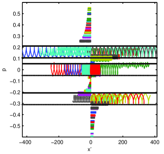
Figure 1: (color online) A phase-space portrait for three resonances. Different colors (shades) describe different trajectories. The horizontal black solid and dashed lines, designate the edges of the resonance chains. The initial conditions were uniformly distributed on the $p$ axis $(x(t=0)=0).$ The system was integrated up-to $t=10^{4}$ (dimensionless variables). At the left figure three non–overlapping resonances are presented, while in the right figure resonances (1) and (2) overlap.

As the number of resonances is increased, we can reach a regime where a large number of these resonances overlap. In this regime we anticipate that the propagation angle of the ray, $p$, could exhibit anomalous diffusion. For the regime when all the resonances overlap, we will compute the diffusion coefficient. The correlation function for the force is

$$C(x_{1},t_{1};x_{2},t_{2}) = \frac{1}{N^{2}}\sum_{n,m=1}^{N}\sum_{i,j=1}^{N}\left\langle A_{m}A_{n}^{\ast}A_{i}^{\ast}A_{j}\right\rangle$$ (48)

$$\times \left\langle(k_{m}-k_{n})(k_{i}-k_{j})\exp\left[{\rm i}\left((k_{m}-k_{n})x_{1}-(\omega_{m}-\omega_{n})t_{1}-(k_{i}-k_{j})x_{2}+(\omega_{i}-\omega_{j})t_{2}\right)\right]\right\rangle.$$

Similarly to the previous section we assume

$$\left\langle A_{m}A_{n}^{\ast}A_{i}^{\ast}A_{j}\right\rangle=\sigma^{4}(\delta_{nm}\delta_{ij}+\delta_{mi}\delta_{nj}).$$ (49)

This reduces equation (48) to

$$C(x_{1}-x_{2},t_{1}-t_{2}) = \frac{\sigma^{4}}{N^{2}}\sum_{n,m=1}^{N}\left\langle(k_{m}-k_{n})^{2}\exp\left[{\rm i}\left((k_{m}-k_{n})(x_{1}-x_{2})-(\omega_{m}-\omega_{n})(t_{1}-t_{2})\right)\right]\right\rangle$$ (50)

$$= \sigma^{4}\int\mathrm{d}k_{1}\int\mathrm{d}k_{2}\,P(k_{1})P(k_{2})(k_{1}-k_{2})^{2}$$

$$\times \exp\left[{\rm i}\left((k_{1}-k_{2})(x_{1}-x_{2})-\frac{1}{2}(k_{1}^{2}-k_{2}^{2})(t_{1}-t_{2})\right)\right]$$

where $P(k)$ is a density of resonances in $k$ space. We used the fact that $k$ and $\omega$ are related by a dispersion relation (40). Using the expression for the diffusion coefficient (17), we obtain

$$D(p) = \frac{1}{2}\int_{-\infty}^{\infty}C(p\tau,\tau)\mathrm{d}\tau=\pi\sigma^{4}\int\mathrm{d}k_{1}\int\mathrm{d}k_{2}\,P(k_{1})P(k_{2})(k_{1}-k_{2})^{2}\delta\left((k_{1}-k_{2})p-\frac{1}{2}(k_{1}^{2}-k_{2}^{2})\right)$$ (51)

$$= \pi\sigma^{4}\int\mathrm{d}k_{1}\int\mathrm{d}k_{2}\,P(k_{1})P(k_{2})(k_{1}-k_{2})^{2}\frac{\delta(k_{1}-(2p-k_{2}))}{|k_{2}-p|}$$

$$= 4\pi\sigma^{4}\int\mathrm{d}k_{2}\,P(2p-k_{2})P(k_{2})|k_{2}-p|.$$

Note that if $P(k)$ has a finite support, than $D(p)$ will also have a finite support. For example for $P(k)=\theta(k_{R}-|k|)/(2k_{R})$, where $\theta(x)$ is a step function, using (51) we compute the diffusion coefficient

$$D(p)=\begin{cases}\frac{\pi\sigma^{4}}{k_{R}^{2}}(k_{R}-|p|)^{2}&|p|\leq k_{R}\\ 0&|p|>k_{R}.\end{cases}$$ (52)

Notice that this expression has finite support, so that the asymptotic relation which leads usually to anomalous diffusion, (25), is not satisfied. In this case a particular form for the potential, which is used in optical realisations of localisation such as Schwartz et al. (2007), leads to sub-diffusive growth of $\langle p^{2}\rangle$. For the case of a large amplitude of the potential, where all resonances overlap, the variation of the momentum of the trajectories is bounded, in accord with the prediction that $D(p)$ has finite support.

In figure 2 we compare a direct numerical evaluation of $\langle p^{2}(t)\rangle$, obtained by averaging solutions of (44) over different initial conditions, with an estimate obtained from a numerical solution of the Fokker-Planck equation

$$\frac{\partial\rho}{\partial z}=\left(\frac{\partial}{\partial p}D(p)\frac{\partial}{\partial p}\right)\rho,$$ (53)

which uses (52) and $k_{R}=0.1$. The classical trajectories all had initial conditions in the resonance chain. A good correspondence is found without any fitting parameter.

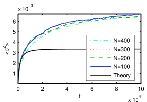
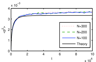
Figure 2: (color online) $\left\langle p^{2}\right\rangle$ as a function of $t$. Dashed gray lines are numerical solution of (44) for $1000$ initial conditions taken from a Gaussian distribution. Different shades and styles of lines designate different $N$ (see legend). The solid think black lines are the numerical solutions of (53) with a diffusion constant given by, (52). The parameters are, $k_{R}=0.1$ and $\sigma=10^{-3}$ for the left figure and $\sigma=10^{-4}$ for the right figure.

IV Summary and Discussion

We have argued that Anderson localization may not be the absence of diffusion in disordered potentials, but rather the absence of anomalous diffusion. More precisely, using the standard argument that at high energies quantum interference effects are negligible, we used effective particles to describe the dynamics, and argued that when Anderson localization is destroyed (due to temporal fluctuations of the potential) the long-time dynamics is determined by a semi-classical approximation. For generic potentials, this semi-classical dynamics exhibits anomalous diffusion in the long-time limit.

Anomalous diffusion in a disordered classical model has previously been studied in several works Golubović et al. (1991); Rosenbluth (1992); Arvedson et al. (2006); Bezuglyy et al. (2006). This work has considered the issues which arise when considering whether this type of anomalous diffusion is also relevant to the breakdown of Anderson localization in optical systems.

The context in which Anderson localization is most readily accessible to experiment is in propagation in a disordered optical potential (refractive index) Schwartz et al. (2007) induced by an optical interference pattern. For this reason, we concentrate upon the case where the potential is quasi-periodic, resulting from the addition of $N$ waves. We discussed the influence of the potential on paraxial propagation of a coherent beam, showing how a semi-classical analysis is related to the Chirikov resonance overlap criterion Zaslavsky and Chirikov (1972); Chirikov (1979) of Hamiltonian dynamics.

Gradually increasing the amplitude it is demonstrated how one transforms from the regime of isolated resonances where no diffusion takes place (Fig. 1, left) to a situation where few resonances overlap (Fig. 1, right) and spreading that involves them is found. When the amplitude is even further increased, such that all the neighboring in momentum resonances overlap and diffusion in momentum is found (Fig. 2).

In the limit as the number $N$ of Fourier components increases, the potential is described in terms of a spectral intensity function $P(k,\omega)$, and the effect of the potential can be modeled by a stochastic equation, describing fluctuations of the momentum $p$ with a diffusion coefficient $D(p)$. We showed how $D(p)$ can be related to the spectral content $P(k,\omega)$ by (22), and how this relation can be interpreted in terms of the Chirikov resonance condition. We also showed that earlier results on anomalous diffusion, (27) and (28) are recovered.

We also considered in some depth the type of potential, such as (43), which arises in optical realizations of Anderson localization such as Schwartz et al. (2007). We showed that the potential which is used in these experiments is non-generic, and leads to $\langle p^{2}(t)\rangle$ being practically bounded, rather than exhibiting anomalous diffusion. This implies that experiments to test the prediction that breaking localisation leads to anomalous diffusion will have to be carefully designed, such that the span of the momentum spectrum of the spatial disorder exceeds the plane-wave spectrum of the initially bounded probe beam, in order to observe anomalous transport.