Squeezing out predictions with leptogenesis from SO(10)

Abstract

We consider the see-saw mechanism within a non-supersymmetric SO(10) model. By assuming the SO(10) quark-lepton symmetry, and after imposing suitable conditions that ensure that the right-handed (RH) neutrino masses are at most mildly hierarchical (compact RH spectrum) we obtain a surprisingly predictive scenario. The absolute neutrino mass scale, the Dirac and the two Majorana phases of the neutrino mixing matrix remain determined in terms of the set of already measured low energy observables, modulo a discrete ambiguity in the signs of two neutrino mixing angles and of the Dirac phase. The RH neutrinos mass spectrum is also predicted, as well as the size and sign of the leptogenesis CP asymmetries. We compute the cosmological baryon asymmetry generated through leptogenesis and obtain the correct sign, and a size compatible with observations.

I Introduction

In the last decade, experiments with solar, atmospheric, reactor and accelerator neutrinos have provided compelling evidences for neutrino oscillations pontecorvo , which imply nonvanishing neutrino masses and mixings. Neutrino oscillation experiments have been measuring with increasing precision the values of the mixing angles and of the mass-squared differences. The value of the absolute neutrino mass scale is still unknown; however, existing limits imply that this scale is bafflingly small, much smaller than those of all the other elementary fermions. The most popular explanation for the neutrino mass suppression is undoubtedly provided by the see-saw mechanism grs which requires the existence of very heavy right-handed (RH) Majorana neutrinos. Fermions with quantum numbers of RH neutrinos, that are singlets under the standard model (SM) gauge group, are found in the spinorial 16 representation of SO(10) georgi ; Fritzsch:1974nn , which therefore provides a quite natural Grand Unified Theory (GUT) framework to embed the see-saw.

The see-saw RH neutrinos also play a key role in leptogenesis fuya ; leptoreview , which is a very appealing scenario to explain the origin of the Baryon Asymmetry of the Universe (BAU). In leptogenesis, the cosmological baryon asymmetry is seeded by an initial asymmetry in lepton number generated in the out-of-equilibrium decay of the RH neutrinos, that is then transferred in part to baryons by means of the $B+L$ violating ‘sphaleron’ interactions, that are non-perturbative SM processes. In SO(10), the order of magnitude of the RH neutrino masses is fixed around the scale of the spontaneous breaking of the $B-L$ U(1) symmetry, and it is consistent with the values of the RH neutrino masses required for successful leptogenesis $M_{R}\sim 10^{11\pm 2}\,$GeV. Indeed, the double role of RH neutrinos in the see-saw and in leptogenesis underlines the importance of deriving information on their mass spectrum.

Recently, an analysis of the relations between the left-handed (LH) neutrino observables (mass-squared differences and mixings) and the RH neutrino spectrum, constrained to be of a compact form (i.e. with masses all of the same order of magnitude) was carried out within the framework of an SO(10)-inspired model Buccella:2010jc , and a scenario for baryogenesis via leptogenesis was also constructed. The study in Ref. Buccella:2010jc was carried out under the simplifying assumption of a vanishing value of the lepton mixing angle $\theta_{13}$, and in the leptogenesis analysis all lepton flavour effects flavour0 ; flavour1 ; flavour2 as well as the effects from the heavier RH neutrinos N2 ; Antusch:2010ms had been neglected. However, recent experimental results hint to a nonvanishing value of $\theta_{13}$ Schwetz:2011zk ; Fogli:2011qn ; GonzalezGarcia:2010er and imply that the assumption $\theta_{13}=0$ should be dropped. The inclusion of flavour effects is also mandatory when leptogenesis occurs below $T\sim 10^{12}\,$GeV, since the one flavour ‘approximation’ is known to give unreliable results. Moreover, in the case of a compact RH spectrum, that is when all the RH neutrino masses fall within a factor of a few, to obtain a trustworthy result it is also necessary to include the asymmetry production and washouts from the two heavier RH neutrinos.

In the present paper we consider a scenario similar to the one in Ref. Buccella:2010jc improving on several points. We fix $\theta_{13}$ to the nonvanishing best fit value given in Ref. GonzalezGarcia:2010er . This in turn implies that the Dirac phase $\delta$ of the Pontecorvo, Maki, Nagakawa and Sakata (PMNS) mixing matrix Maki:1962mu ; Bilenky:1978nj enters all the equations, and in particular contributes to the leptogenesis CP asymmetries. Most importantly, we clarify how the conditions ensuring a compact RH neutrino spectrum have consistent solutions only for $\delta\neq 0$, and how the corresponding solutions yield a surprisingly predictive scenario in which all the yet unknown low energy parameters, namely the LH neutrino mass scale $m_{1}$ and the three PMNS CP violating phases $\delta,\,\alpha$ and $\beta$, remain determined in terms of already measured quantities, modulo a few signs ambiguities. In the high energy sector, the RH neutrino spectrum is also predicted. The crucial test of the scenario is then the computation of the baryon asymmetry yield of leptogenesis. We include lepton flavour effects flavour0 ; flavour1 ; flavour2 in our analysis and argue that they are crucial to evaluate correctly the baryon asymmetry. Most importantly, the high level of predictability of our framework allows to predict both the size and the sign of the BAU. By requiring agreement with observations, we are then able to solve almost completely the residual signs ambiguities.

The paper is organized as follows. In Section II we describe the SO(10) framework and spell out the quark-lepton symmetry assumption. In Section III we discuss the constraining conditions that ensure a compact spectrum for the RH neutrinos. In spite of quark-lepton symmetry a compact form is achieved, and with a sufficiently large scale not to conflict with the Davidson-Ibarra bound that, within the $SO(10)$ see-saw, often vetoes successful baryogenesis via leptogenisis. In Section IV we confront our scenario with the set of measured low energy neutrino observables, and we work out predictions for the absolute scale of neutrino masses $m_{1}$, for the PMNS CP violating phases $\delta,\,\alpha,\,\beta$ and for the RH neutrino mass matrix. In Section V we calculate the various CP asymmetries in RH neutrino decays, we briefly discuss the procedure followed to estimate the baryon asymmetry yield of leptogenesis and stress how a proper treatment of flavour effects is crucial for obtaining reliable estimates for the different cases. Finally in Section VI we discuss our results and draw the conclusions.

II $\mathbf{SO(10)}$ GUT and quark-lepton symmetry

We work in a non-supersymmetric grand unified SO(10) model. We assume three fermion families whose left-handed (LH) states are assigned to a ${\bf 16}$ spinorial representation of SO(10), which thus contains all the SM fermion and antifermion states of the same chirality. In addition, the ${\bf 16}$ includes one $SU(2)$ singlet neutrino for each family. All elementary fermions of opposite chirality (RH) are assigned to the conjugate representation $\overline{\mathbf{16}}$. Fermion masses are generated by Yukawa terms of the form:

$$Y_{ij}\cdot\mathbf{16}_{i}\,H^{\dagger}\,\mathbf{16}_{j}+{\rm h.c.}$$ (1)

where $Y$ is a $3\times 3$ matrix of Yukawa couplings with indexes in family space, and $H$ denotes a multiplet of scalar (Higgs) bosons. The tensor product of the fermion representations in eq. (1) gives

$${\bf 16}\times{\bf 16}={\bf 10}_{s}+{\bf 126}_{s}+{\bf 120}_{a}$$ (2)

where the subscripts $s,a$ refer to the symmetric and antisymmetric nature of the representation in the family indexes. Thus, to make the Yukawa term in eq. (1) an SO(10) singlet, $H$ must be assigned to a $\bf{10}$, to a $\bf{126}$, or to a $\bf{120}$. Clearly, for $\bf{10}$ and $\bf{126}$, that match the two symmetric fragments of the tensor product, the Yukawa matrix $Y$ is symmetric, while for the $\bf{120}$ it is antisymmetric.

In the present work we consider Yukawa terms involving only the $\bf{10}$ and $\bf{126}$ that are already needed for the gauge symmetry breaking pattern (the $\bf{126}$ is also needed to generate Majorana masses for the see-saw RH neutrinos) and we exclude Yukawa couplings with the $\bf{120}$ which would imply a departure from minimality.

We adopt the following SO(10) breaking pattern; we also indicate the set of Higgs $SO(10)$ representations needed for each step

$$SO(10) \xrightarrow{{\bf 210}} SU(2)_{L}\otimes SU(2)_{R}\otimes SU(4)$$ (3)

$$\xrightarrow{{\bf 126}} SU(2)_{L}\times U(1)_{Y}\times SU(3)_{C}$$

$$\xrightarrow{{\mathbf{126},\>\,\mathbf{10}}} SU(3)_{C}\times U(1)_{Q}$$

The first step in this chain is a breaking to a maximal subgroup of $SO(10)$, the intermediate Pati-Salam group $SU(2)_{L}\otimes SU(2)_{R}\otimes SU(4)$patisalam . Let us list explicitly useful branching rules for $SO(10)\to SU(2)_{L}\otimes SU(2)_{R}\otimes SU(4)$:

$$\mathbf{210} \supset (\mathbf{1},\mathbf{1},\mathbf{1})\oplus\dots$$

$$\mathbf{126} = (\mathbf{1},\mathbf{1},\mathbf{6})\oplus(\mathbf{3},\mathbf{1},\mathbf{10})\oplus(\mathbf{1},\mathbf{3},\mathbf{\overline{10}})\oplus(\mathbf{2},\mathbf{2},\mathbf{15})$$

$$\mathbf{16} = (\mathbf{2},\mathbf{1},\mathbf{4})\oplus(\mathbf{1},\mathbf{2},\mathbf{\overline{4}})$$

$$\mathbf{16}\otimes\mathbf{16} \supset (\mathbf{1},\mathbf{3},\mathbf{\overline{10}})\oplus\dots$$ (4)

The $SU(2)_{L}\otimes SU(2)_{R}\otimes SU(4)$ singlet in the $\mathbf{210}$ is responsible for the first breaking at the GUT scale.

The $\mathbf{126}$ then breaks $SU(2)_{L}\otimes SU(2)_{R}\otimes SU(4)\to SU(2)_{L}\otimes U(1)_{Y}\otimes SU(3)_{C}$ at an intermediate scale $\Lambda_{R}$, that we assume to be around $10^{11}\,$GeV. The relevant component that triggers the breaking is $(\mathbf{1},\mathbf{3},\mathbf{\overline{10}})$ since the $\mathbf{10}$ of $SU(4)$ contains an $SU(3)$ singlet. The other components, $(\mathbf{3},\mathbf{1},\mathbf{10})$ and $(\mathbf{2},\mathbf{2},\mathbf{15})$ would break $SU(2)_{L}$, while $(\mathbf{1},\mathbf{1},\mathbf{6})$ would break colour. The RH neutrino $N$, together with all the other SM $SU(2)_{L}$ singlet fields, is contained in $(\mathbf{1},\mathbf{2},\mathbf{\overline{4}})$, and thus the bilinear $N\cdot N$ belongs to the fragment displayed in the last line, which is the only one suited to build up a gauge invariant term when coupled to the intermediate gauge symmetry breaking component $(\mathbf{1},\mathbf{3},\mathbf{10})$ of the $\mathbf{\overline{126}}$ Higgs multiplet. We can also decompose $SO(10)$ according to $SO(10)\supset SU(5)\,\otimes\,U(1)\supset SU(5)$. With respect to $SU(5)$:

$$\mathbf{126}=\mathbf{1}+\mathbf{\overline{5}}+\mathbf{10}+\mathbf{\overline{15}}+\mathbf{45}+\mathbf{\overline{50}}\,.$$ (5)

Of these representations only the $\mathbf{1}$, $\mathbf{\overline{5}}$, and $\mathbf{45}$ have neutral colour singlet Higgs components that can have nonzero vacuum expectation values if $U(1)_{em}\times SU(3)_{C}$ has to remain unbroken. $N$ is a singlet with respect to $SU(5)$ and so it is $N\cdot N$; therefore, it is the $SU(5)$ singlet in $\mathbf{\overline{126}}$ that couples to $N\cdot N$ and gives an invariant mass of the order of the intermediate scale to $N$. In terms of the intermediate representations, it is $(\mathbf{1},\mathbf{3},\mathbf{\overline{10}})$ in last line of Eq. (II), that must contain an SU(5) singlet.

As regards the fermion masses, if they originate only from vacuum expectation values (vevs) of scalars in the $\bf{10}$, the following relations hold:

$$m_{D}=m_{u},\qquad\qquad m_{e}=m_{d},$$ (6)

where $m_{D}$ is the neutrino Dirac mass matrix, and $m_{u}$, $m_{d}$ and $m_{e}$ are respectively the mass matrices for the up and down quarks and charged leptons. The two relations in eq. (6) are sometimes referred to as quark-lepton symmetry; they imply for each generation the GUT scale prediction $m_{e_{i}}/m_{d_{i}}=1$ (with $i=1,2,3$ a generation index) which however, after including renormalization group corrections, agrees with observations only for the third generation ($b$-$\tau$ unification) but is badly violated for the first and second generations. If instead quark and lepton masses originate from one or more $\bf{126}$ (that however should be different from the $\bf{126}$ that breaks the gauge symmetry) the following relations hold:

$$m_{D}=-3m_{u},\qquad\qquad m_{e}=-3m_{d}\,.$$ (7)

The factor of $-3$ is a colour factor between leptons and quarks; it is reminiscent of the Georgi and Jarlskog mechanism Georgi:1979df , which in SU(5), when it appears in a family dependent way, allows to circumvent the prediction of unification for the first two families yielding $m_{\mu}/m_{s}\neq m_{e}/m_{d}\neq 1$ while preserving $m_{\tau}/m_{b}=1$. In SU(5) the discrepancy with the observed values of the down-quarks and charged lepton masses can in fact be weakened by assuming that the Yukawa coupling of the second generation to itself involves a $\mathbf{45}$ of SU(5) scalars, instead of the usual $\mathbf{\bar{5}}$, yielding mass ratios

$$|m_{\mu}/m_{s}|=|m_{d}/m_{e}|=3$$ (8)

which are in better agreement with the measured values. Now, under SO(10) $\to$ SU(5)$\,\times\,$U(1) the $\bf{126}$ contains precisely a $\mathbf{45}$ which, as Harvey, Ramond and Reiss showed Harvey:1980je ; Harvey:1981hk , allows to implement the same mechanism also in SO(10).

In our SO(10) model we assume that the SM $SU(2)_{L}$ Higgs doublet is a combination of representations in the $\bf{10}$ and $\bf{126}$ of SO(10). While this allows to account for non-unification for the down-quark and charged lepton masses of the two lightest families, it still predicts an approximate quark-lepton symmetry, that is $m_{e}\sim m_{d}$ are in any case connected by coefficients of order 1. As regards the neutrino Dirac mass matrix, for definiteness we will stick to the simpler relation in eq. (6), which can coexist with eq. (7) for $m_{\mu,s}$, $m_{e,d}$ if the $u$-$\nu$ sector masses are dominated by the $\mathbf{10}$ vevs. We also assume that, in the diagonal basis for the down-quarks and charged leptons mass matrices, the unitary rotation $V_{L}$ that diagonalizes the symmetric matrix $m_{D}$ coincides with the Cabibbo-Kobayashi-Maskawa (CKM) rotation that diagonalizes $m_{u}$. Namely we assume as a working hypothesis:

$$m_{D}=m_{u}\qquad{\rm and}\qquad V_{L}=V_{CKM}\,.$$ (9)

We stress at this point that our results do not depend in any crucial way on the precise form of the quark-lepton relations, and the ansatz eq. (9) is adopted here only for the sake of simplicity. However, the possibility of constructing a predictive framework does depend on the fact that in SO(10) a precise relation between $m_{D}$ and $m_{u}$ and $V_{L}$ and $V_{CKM}$ exists, which naturally follows from fermions unification within a single irreducible representation of the group. In fact, once the details of the symmetry breaking pattern and of the fermion couplings to the $\mathbf{10}$ and $\mathbf{126}$ are given, a quark-lepton mass relation remains in any case fixed, and in particular a highly hierarchical spectrum for the eigenvalues of $m_{D}$ is a straightforward consequence of the SO(10) GUT framework (see also Ref. Akhmedov:2003dg ). As regards the full $6\times 6$ mass matrix of the neutral sector, recalling that symmetric Yukawa matrices imply that $m_{D}^{T}=m_{D}$, it can be written as

$$M=\left(\begin{array}[]{cc}0&m_{D}\\ m_{D}&M_{R}\end{array}\right)\,,$$ (10)

where $m_{D}$ and $M_{R}$ receive respectively contributions from the following vevs:

$$m_{D}\sim\langle\mathbf{10}+\mathbf{126}\rangle_{\Lambda_{EW}}\,,\qquad\qquad M_{R}\sim\langle\mathbf{126}\rangle_{\Lambda_{R}}\,,$$ (11)

where the $\mathbf{126}$ contributing to $M_{R}$ has a vev ${\cal O}(\Lambda_{R})\gg\Lambda_{EW}$ along the $SU(5)$ singlet component.

III Compact RH neutrino spectrum

The hierarchy $\Lambda_{EW}/\Lambda_{R}\ll 1$ between the two types of vevs in eq. (11) enforces the see-saw mechanism, and, after diagonalizing the matrix (10), one obtains the light neutrino mass matrix $m_{\nu}$ from the seesaw formula that, with $m_{D}^{T}=m_{D}$, reads:

$$m_{\nu} \simeq -m_{D}\,M_{R}^{-1}\,m_{D}\,.$$ (12)

Inverting the seesaw formula (12) gives

$$M_{R}\simeq-m_{D}\,m_{\nu}^{-1}\,m_{D},$$ (13)

which shows that one can obtain information on $M_{R}$ by using the available experimental data on $m_{\nu}$, and assuming quark-lepton symmetry for $m_{D}$.

Quark-lepton symmetry however, renders problematic the implementation of the mechanism of baryogenesis via leptogenesis within the SO(10) see-saw Falcone:2000ib ; Nezri:2000pb . This is due to the two factors of $m_{D}$ in eq. (13) that in general yield a very hierarchical spectrum for the RH neutrinos. In fact, by fixing the intermediate scale $\Lambda_{R}$ around $10^{11}\,$GeV, the lightest RH state $N_{1}$, which is generally the main one responsible for generating a lepton asymmetry, acquires a mass $M_{R_{1}}\ll 10^{9}\,$GeV, that is well below the Davidson-Ibarra (DI) limit di which gives the benchmark to guarantee a sufficient production of lepton asymmetry from RH neutrino decays. There are basically two ways out to this problem. The first one relies on the fact that under certain conditions leptogenesis can also proceed via the decays of the two heavier RH neutrinos N2 , whose masses remain well above the DI bound. Refs. oscar ; db1 ; Abada:2008gs ; DiBari:2008mp ; DiBari:2010ux ; Blanchet:2010td present specific realizations of this possibility. The second way out relies on the possibility of enhancing resonantly the CP asymmetries PU , which allows to evade completely the DI bound, but requires that at least one pair of RH neutrinos is highly degenerate in mass. In this paper we explore a third possibility, namely that in spite of the quark-lepton symmetry, the RH neutrino spectrum could still turn out to be of a compact form Buccella:2010jc that is, characterized by at most mildly hierarchical mass eigenvalues, all with values within the range $10^{11\pm 2}\,$GeV which is the optimal one for leptogenesis. Clearly, such a possibility would avoid from the start the problem of a too light $N_{1}$. Let us see in detail how this possibility can be implemented.

III.1 Conditions for a compact $N_{i}$ spectrum

A generic Dirac neutrino mass $m_{D}$ can be diagonalized by means of a biunitary transformation with two unitary matrices $V_{L}$ and $V_{R}$, that is $m_{D}=V_{L}^{\dagger}m_{D}^{diag}V_{R}$. However, due to the assumed specific symmetry breaking pattern, in our model $m_{D}$ is symmetric, and in this case there exists (Takagi factorization Takagi ) a single unitary matrix $V_{L}$ such that

$$m_{D} = V_{L}^{\dagger}m_{D}^{diag}V_{L}^{*},$$ (14)

where $m_{D}^{diag}={\rm diag}\left(m_{D1},m_{D2},m_{D3}\right)$ is diagonal with real and non-negative eigenvalues. It follows that the RH neutrino mass matrix can be written in the form

$$M_{R} = -V_{L}^{\dagger}m_{D}^{diag}A\,m_{D}^{diag}V_{L}^{*}\,,$$ (15)

where we have introduced the symmetric matrix

$$A=V_{L}^{\star}\,m_{\nu}^{-1}\,V_{L}^{\dagger}\,.$$ (16)

On a naturalness ground, from the current knowledge about the light neutrino mass matrix $m_{\nu}$, in the basis where charged lepton mass matrix is diagonal one would expect that the elements of $A$ are at most mildly hierarchical. Then, if $m_{D}^{diag}$ is hierarchical as implied by quark-lepton symmetry, we would generally obtain a hierarchical RH neutrino spectrum. Therefore only a quite specific structure of the $A$ matrix in eq. (16) can enforce the conditions that ensure that the RH neutrino spectrum is compact. To illustrate this issue, let us recall that we are working under the assumption of quark-lepton symmetry eq. (9) which implies in particular that in the basis where the mass matrix of the charged leptons and of the down-type quarks are diagonal $V_{L}=V_{CKM}$. Although the results in Sections IV and V are obtained with the assumption $V_{L}=V_{CKM}$, to write down reasonable analytical expressions for the RH neutrino mass spectrum in this section, we will set in first approximation $V_{L}=I_{3\times 3}$ (where the $I_{3\times 3}$ is the $3\times 3$ identity matrix). Eq. (15) then gives

$$M_{R} \approx -\left(\begin{array}[]{ccc}A_{11}m_{D1}^{2}&A_{12}m_{D1}m_{D2}&A_{13}m_{D1}m_{D3}\\ A_{12}m_{D1}m_{D2}&A_{22}m_{D2}^{2}&A_{23}m_{D2}m_{D3}\\ A_{13}m_{D1}m_{D3}&A_{23}m_{D2}m_{D3}&A_{33}m_{D3}^{2}\end{array}\right)\,,$$ (20)

with $A\approx m_{\nu}^{-1}$ (recall that because $A$ is symmetric $A_{ij}=A_{ji}$). Quark-lepton symmetry implies $m_{D3}\gg m_{D2}\gg m_{D1}$, which suggests that a generically compact RH spectrum would result if

$$\left|\frac{A_{33}}{A_{22}}\right|\mbox{${~{}\raise 2.5pt\hbox{$<$}\kern-6.99997pt\lower 2.5pt\hbox{$\sim$}~{}}$}\frac{m_{D2}^{2}}{m^{2}_{D3}}\qquad\qquad{\rm and}\qquad\qquad\left|\frac{A_{23}}{A_{22}}\right|\mbox{${~{}\raise 2.5pt\hbox{$<$}\kern-6.99997pt\lower 2.5pt\hbox{$\sim$}~{}}$}\frac{m_{D2}}{m_{D3}}$$ (21)

since, if this were the case, all the hierarchically large entries in $M_{R}$ would be sufficiently suppressed (notice that the $M_{R}$(1,3) and $M_{R}$(2,2) elements of eq. (20) are non-hierarchical because from the light neutrino mass matrix we expect $A_{22}\sim A_{13}$ and from the quark-lepton symmetry we expect $m_{D1}m_{D3}\sim m_{D2}^{2}$). However, in this paper we will assume the more restrictive condition:

$$\left|\frac{A_{33}}{A_{11}}\right|\mbox{${~{}\raise 2.5pt\hbox{$<$}\kern-6.99997pt\lower 2.5pt\hbox{$\sim$}~{}}$}\frac{m_{D1}^{2}}{m^{2}_{D3}}\ll 1,\qquad\qquad\left|\frac{A_{23}}{A_{11}}\right|\mbox{${~{}\raise 2.5pt\hbox{$<$}\kern-6.99997pt\lower 2.5pt\hbox{$\sim$}~{}}$}\frac{m_{D1}^{2}}{m_{D2}m_{D3}}\ll 1,\qquad\qquad$$ (22)

since they are needed to justify the simplifying approximation in eq. (23) below. The interest in exploring a scenario in which the two conditions in eq. (22) are realized stems from the fact that it is quite likely that an $A$-matrix of this form would render leptogenesis a viable mechanism to explain the BAU within the SO(10) seesaw framework. In this paper, we will not speculate on the possible origin of the two relations in eq. (22), nor we will attempt to reproduce them by starting from a suitable fundamental Lagrangian, and thus the possibility that such a pattern could arise basically relies only on the fact that similar hierarchies do exist among quantities related to the Yukawa coupling sector. In fact, we believe that building up a theoretical justification for $A_{33}/A_{11},\,A_{23}/A_{11}\ll 1$ could be equally difficult than explaining the mass hierarchies of the charged fermions, which is a long standing unsolved problem in particle physics. We will, however, prove that as long as $\theta_{13}$ is nonvanishing, imposing such relations is a technically consistent procedure, in the sense that they can be always fulfilled, regardless of the specific types of quark-lepton symmetry relations assumed. If $A_{23}$ and $A_{33}$ are negligible with respect to all the other entries, we can set in first approximation

$$A_{23}=A_{33}=0\,.$$ (23)

As we will see, from these two conditions it follows that, besides obtaining a compact RH spectrum, two eigenvalues in $M_{R}$ will actually be close to degenerate. In general, the degeneracy of pairs of $M_{R}$ eigenvalues represents an interesting situation for leptogenesis, since it can allow for resonant enhancement of the CP asymmetries. Although we will find that, eventually, conditions eq. (23) are not sufficient to bring the dynamics of leptogensis fully within the resonant regime, it is still worth studying which class of general conditions for $A$ could yield a pair of eigenvalues very close in mass.

The eigenvalues $\lambda$ of $M_{R}$ in eq. (20) are given by the solutions to the characteristic cubic equation

$$\lambda^{3}+b\lambda^{2}+c\lambda+d = 0,$$ (24)

with

$$b = A_{11}m_{D1}^{2}+A_{22}m_{D2}^{2}+A_{33}m_{D3}^{2},$$

$$c = \left(A_{11}A_{22}-A_{12}^{2}\right)m_{D1}^{2}m_{D2}^{2}+\left(A_{11}A_{33}-A_{13}^{2}\right)m_{D1}^{2}m_{D3}^{2}+\left(A_{22}A_{33}-A_{23}^{2}\right)m_{D2}^{2}m_{D3}^{2},$$

$$d = \left(2A_{12}A_{13}A_{23}+A_{11}A_{22}A_{33}-A_{13}^{2}A_{22}-A_{12}^{2}A_{33}-A_{23}^{2}A_{11}\right)m_{D1}^{2}m_{D2}^{2}m_{D3}^{2}.$$ (25)

The necessary condition for two eigenvalues being equal is that the discriminant of eq. (24) vanishes. We can write down the discriminant as follows

$$\Delta = b^{2}c^{2}-4c^{3}-4b^{3}d+18bcd-27d^{2}$$ (26)

$$\approx \left(A_{23}^{2}-A_{22}A_{33}\right)^{2}m_{D2}^{4}m_{D3}^{4}\left[A_{22}^{2}m_{D2}^{4}+A_{33}^{2}m_{D3}^{4}+2\left(2A_{23}^{2}-A_{22}A_{33}\right)m_{D2}^{2}m_{D3}^{2}\right]\,,$$

where in the second line we have expanded up to first order in $\frac{m_{D1}}{m_{D3}}\sim\frac{m_{u}}{m_{t}}$. We have $\Delta=0$ if

$$A_{23}^{2} = A_{22}A_{33},\;\;\;\;{\rm or}\;\;\;\;A_{23}^{2}=-\left(\frac{A_{22}m_{D2}^{2}-A_{33}m_{D3}^{2}}{2m_{D2}m_{D3}}\right)^{2}.$$ (27)

We will consider only the first possibility, that involves solely elements of the matrix $A$. We then see that if $A_{23}\,,A_{33}\approx 0$ or alternatively $A_{23},\,A_{22}\approx 0$, quasi degeneracy of two RH neutrino masses results. Notice that the first condition also satisfies eq. (22), and then it will result in a compact spectrum, in contrast, as we will see in the following, the second condition will yield a hierarchical spectrum. Before dealing with these two cases in detail, let us remark that without loss of generality, it is convenient to work in the basis where the RH neutrino mass matrix $M_{R}$ is diagonal. Since $M_{R}$ is symmetric, it can be brought to diagonal form $M_{R}^{diag}={\rm diag}(M_{1},M_{2},M_{3})$ with real and positive entries by means of a unitary matrix $W$:

$$M_{R}^{diag} = W^{\dagger}M_{R}W^{*}\,.$$ (28)

In this basis we redefine the Dirac mass matrix as follows

$$\hat{m}_{D} = m_{D}W^{*}.$$ (29)

From now on we will always work in this basis.

III.1.1 Case 1: $A_{23}=0$, $A_{33}=0$

In this case, we solve eq. (24) and expand the eigenvalues up to first order in $\frac{m_{D1}}{m_{D3}}$; we obtain the following spectrum for the RH neutrinos

$$M_{1} = \left|A_{22}\right|m_{D2}^{2},$$

$$M_{2} = \left|A_{13}\right|m_{D1}m_{D3},$$

$$M_{3} = \left|A_{13}\right|m_{D1}m_{D3}.$$ (30)

With the reasonable assumption that $\left|A_{13}\right|$ and $\left|A_{22}\right|$ are not very hierarchical, we see that it is possible to have $M_{1}\simeq M_{2,3}$ and, depending on the values of $m_{D}^{diag}$ renormalized at the leptogenesis scale, both mass orderings $M_{1}<M_{2,3}$ or $M_{2,3}<M_{1}$ are possible. In ref. Buccella:2010jc only the $M_{1}<M_{2,3}$ ordering was considered, a vanishing $\theta_{13}$ was assumed, and both lepton flavour and heavier RH neutrino effects in leptogenesis had been ignored. Instead, as we will show, the ordering $M_{2,3}<M_{1}$ can indeed occur, $\theta_{13}\neq 0$ is a crucial condition to ensure the existence of solutions for the compact spectrum conditions, and as regards the lepton flavour and heavy RH neutrino effects, they must be included in order to obtain successful leptogenesis, and to guarantee that the result is reliable.

III.1.2 Case 2: $A_{23}=0$, $A_{22}=0$

In this case, by proceeding as before up to first order in $\frac{m_{D1}}{m_{D3}}$, we obtain the spectrum

$$M_{1} = \left|A_{33}\right|m_{D3}^{2},$$

$$M_{2} = \left|A_{12}\right|m_{D1}m_{D2},$$

$$M_{3} = \left|A_{12}\right|m_{D1}m_{D2}.$$ (31)

Assuming also in this case that $\left|A_{12}\right|$ and $\left|A_{33}\right|$ are not exceedingly hierarchical implies $M_{1}\gg M_{2,3}$. Of course in this case, since the large contributions from $m_{D3}$ are not suppressed, we do not expect to obtain a compact RH spectrum. Nevertheless, in principle leptogenesis could still proceed at a scale $M_{2,3}\ll\Lambda_{R}$ thanks to the asymmetries generated in the decays of the two quasi degenerate states $N_{2,3}$. Eventually however, we will find that in Case 2 on the one hand leptogenesis is unable to produce a sufficient baryon asymmetry, and on the other hand for the heaviest RH neutrino we always obtain $M_{3}\mbox{${~{}\raise 2.5pt\hbox{$>$}\kern-6.99997pt\lower 2.5pt\hbox{$\sim$}~{}}$}10^{14}\,$GeV which, under the requirement of perturbative Yukawa couplings, is in conflict with $SO(10)$ gauge coupling unification which instead suggests an intermediate vevs scale of order $10^{11}\,$GeV Bertolini:2009qj (see however Bertolini:2012im for viable scenarios with an intermediate scale as high as $10^{14}$ GeV).

IV Relation with low energy observables

We have seen that by assuming conditions eq. (23) we have forcibly ended up with a quasi degenerate pair of RH eigenvalues. Before proceeding, let us stress that while setting the values of $A_{23}$ and $A_{23}$ to an exact zero has the virtue of simplifying the analysis, a generic compact RH neutrino spectrum can be obtained by fixing instead their values to any sufficiently small number as dictated by eq. (21). Doing this would lift the quasi degeneracy, but would still yield similar results. We will return to this point in Section V. One important point is that requiring that the matrix $A$ satisfies some specific conditions gets reflected in specific relations between the low energy observables, and yields an enhanced level of predictability for the SO(10) model. Before studying which type of relations arise, it is useful to carry out a quick counting of the fundamental free parameters of the theory, and list the phenomenological constraints that they should satisfy. The structure of the two symmetric matrices $m_{D}$ and $M_{R}$ is determined by two corresponding sets of fundamental Yukawa couplings between the fermion fields in the $\mathbf{16}$ and the Higgs fields respectively with vevs $\sim\Lambda_{EW}$ and $\sim\Lambda_{R}$. This amounts to $6+6+1=13$ real parameters corresponding to the two symmetric Yukawa matrices plus the ratio $\Lambda_{EW}/\Lambda_{R}$ which determines the seesaw suppression of neutrino masses, or in other words their absolute scale. Under the assumption of quark-lepton duality (see eq. 9), the values of the 13 real parameters are constrained by the following observables in the up-type quark and neutrino sectors: the three quark masses $m_{u},\,m_{c},\,m_{t}$, the two neutrino mass-squared differences $\Delta m^{2}_{12},\,\Delta m^{2}_{23}$, the three CKM mixing angles $\theta_{12}^{\prime},\,\theta_{23}^{\prime},\,\theta_{13}^{\prime}$ and the three PMNS mixing angles $\theta_{12},\,\theta_{23},\,\theta_{13}$, which add up to a total of $11$ constraints. Now, imposing on the complex elements of the matrix $A$ two additional conditions, e.g. $A_{23}=A_{33}=0$ (or any other pair of conditions), implies that the set of 13 real fundamental parameters must satisfy two additional requirements, that in our case read ${\rm Re}(A_{23})={\rm Re}(A_{33})=0$. Thus the parameter space of the model remains completely determined allowing to obtain a quantitative prediction for the absolute neutrino mass scale $m_{\nu_{1}}$. As regards the constraints on imaginary quantities, there are many fundamental complex phases, and only one measured observable, the CKM phase $\delta^{\prime}$. Nevertheless, as we will see, the structure of the conditions implies nontrivial relations between $\delta^{\prime}$ and the three PMNS phases $\alpha,\beta$ and $\delta$.

In the following we assume a hierarchical and normally ordered spectrum for the light neutrino masses $m_{\nu}^{diag}={\rm{diag}}(m_{1},m_{2},m_{3})$ with

$$m_{1}<m_{2}<m_{3},$$ (32)

which is justified by the assumption of quark-lepton symmetry eq. (9). In the basis where charged lepton mass matrix is diagonal, the PMNS mixing matrix $U_{PMNS}$ diagonalizes the effective neutrino mass matrix

$$m_{\nu}=U_{PMNS}^{\star}m_{\nu}^{diag}U_{PMNS}^{\dagger}.$$ (33)

We adopt for $U_{PMNS}$ the standard parametrization in terms of 3 angles and three complex phases:

$$U_{PMNS} = \left(\begin{array}[]{ccc}c_{12}c_{13}&s_{12}c_{13}&s_{13}e^{-i\delta}\\ -s_{12}c_{23}-c_{12}s_{23}s_{13}e^{i\delta}&c_{12}c_{23}-s_{12}s_{23}s_{13}e^{i\delta}&s_{23}c_{13}\\ s_{12}s_{23}-c_{12}c_{23}s_{13}e^{i\delta}&-c_{12}s_{23}-s_{12}c_{23}s_{13}e^{i\delta}&c_{23}c_{13}\end{array}\right)\times{\rm diag}\left(1,e^{i\alpha},e^{i\beta}\right)\,.$$ (37)

Here $c_{ij}=\cos\theta_{ij}$ and $s_{ij}=\sin\theta_{ij}$, with $i$ and $j$ labeling families that are coupled through that angle ($i,j=1,2,3$). Note that since the computation of the leptogenesis CP asymmetries involves several interfering amplitudes, the angles $\theta_{ij}$ cannot be restricted to the first quadrant, except for $\theta_{13}$ that can be taken to be positive once the CP phase $\delta$ is allowed to range between $-\pi$ and $\pi$.

According to the quark-lepton symmetry ansatz eq. (9), in the numerical analysis we take $V_{L}=V_{CKM}$, and accordingly we parametrize $V_{L}$ with three angles and one phase, with a structure analogous to the first matrix on the right-hand-side (RHS) of eq. (37), distinguishing the angles and phase with a prime superscript: $s_{12}^{\prime},\,s_{23}^{\prime},\,s_{13}^{\prime},\,\delta^{\prime}$. The following discussion, however, is based on analytical expressions that get largely simplified by writing $V_{L}$ in the approximate Cabibbo-like form:

$$V_{L}^{(C)}=\left(\begin{array}[]{ccc}\cos\theta_{C}&\sin\theta_{C}&0\\ -\sin\theta_{C}&\cos\theta_{C}&0\\ 0&0&1\end{array}\right)\,.$$ (38)

We will then write our formulae in this approximation, keeping in mind however, that the full expressions have been used to obtain the numerical results.

The matrix $A$ eq. (16) can be expressed in terms of the observables $V_{L}$, $U_{PMNS}$ and $m_{\nu}^{diag}$ as

$$A=\left(V_{L}U_{PMNS}^{\star}\right)^{\star}\,\frac{1}{m_{\nu}^{diag}}\,\left(V_{L}U_{PMNS}^{\star}\right)^{\dagger}\,.$$ (39)

In the approximation $V_{L}=V_{L}^{(C)}$, the conditions ${A}_{23}={A}_{33}=0$ yield the following two relations:

$$\frac{m_{2}}{m_{1}}\,e^{-2i\alpha} = -\frac{\left(c_{12}s_{23}+e^{i\delta}s_{12}s_{13}c_{23}\right)\left[s_{c}c_{12}s_{13}s_{23}+e^{i\delta}(s_{c}s_{12}c_{23}-c_{c}c_{12}c_{13})\right]}{\left(-s_{12}s_{23}+e^{i\delta}c_{12}s_{13}c_{23}\right)\left[-s_{c}s_{12}s_{13}s_{23}+e^{i\delta}(c_{c}s_{12}c_{13}+s_{c}c_{12}c_{23})\right]}\,,$$ (40)

$$\frac{m_{3}}{m_{1}}\,e^{-2i\beta} = \frac{c_{13}c_{23}\left[s_{c}s_{12}c_{23}+c_{12}\left(-c_{c}c_{13}+s_{c}e^{-i\delta}s_{13}s_{23}\right)\right]}{\left(-s_{12}s_{23}+e^{i\delta}c_{12}s_{13}c_{23}\right)\left(s_{c}c_{13}s_{23}+c_{c}e^{i\delta}s_{13}\right)}.$$ (41)

where $s_{c},c_{c}=\sin\theta_{C},\cos\theta_{C}$.

We see that by taking the absolute values of eqs. (40)-(41) we obtain two conditions that do not depend on the Majorana phases $\alpha,\beta$ (and are also even functions of $\delta$ that depend only on its cosine). We can further eliminate $m_{2}$ and $m_{3}$ by using their relations with the solar and atmospheric mass-squared differences: $m^{2}_{2}=m^{2}_{1}+\Delta m^{2}_{s}$ and $m^{2}_{3}=m^{2}_{1}+\Delta m^{2}_{a}$, obtaining:

$$1+\frac{\Delta m^{2}_{s}}{m_{1}^{2}} = f_{12}([\theta_{C},\theta_{12},\theta_{23},\theta_{13}];\cos\delta),$$ (42)

$$1+\frac{\Delta m^{2}_{a}}{m_{1}^{2}} = f_{23}([\theta_{C},\theta_{12},\theta_{23},\theta_{13}];\cos\delta)\,.$$ (43)

The absolute neutrino mass scale $m_{1}$ appearing on the LHS of these equations represents the first unknown. On the RHS, $f_{12}$ and $f_{23}$ are two known (although non-transparent) functions of known mixing angles (that are listed within the squared brackets) and of the cosine of the second unknown, that is the Dirac phase $\delta$. These two equations might or might not have physical solutions (for example, given that $\Delta m^{2}_{s}>0$, in case the RHS of the first equation remains $\leq 1$ for all values of $\delta$, there are no physically acceptable solutions). If solutions exists, these will corresponds to specific values of $m_{1}$ and of $\delta$ with uncertainties determined by the experimental errors on the mixing angles.

As regards the conditions on the complex arguments of eqs. (40)-(41), they have the form

$$\alpha=g_{12}([\theta_{C},\theta_{12},\theta_{23},\theta_{13},\Delta m_{s}^{2}];\delta,m_{1}),$$ (44)

$$\beta=g_{23}([\theta_{C},\theta_{12},\theta_{23},\theta_{13},\Delta m_{a}^{2}];\delta,m_{1}),$$ (45)

where $g_{12}$ and $g_{13}$ are again known functions, and thus $\alpha$ and $\beta$ can be determined in terms of $m_{1}$, $\delta$ and of the known mixing angles and mass squared differences. This completes the determination of all the low energy observables in terms of measured quantities, and through eq. (15) also fixes the RH neutrinos mass spectrum.

Quark sector		Neutrino sector
$m_{u}(\Lambda)$	$0.00067\>{\rm GeV}$	$\Delta m^{2}_{21}(\Lambda)$	$11.86\times 10^{-5}\>{\rm eV}^{2}$
$m_{c}(\Lambda)$	$0.327\ \ {\rm GeV}$	$\Delta m^{2}_{31}(\Lambda)$	$3.84\times 10^{-3}\>{\rm eV}^{2}$
$m_{t}(\Lambda)$	$99.1\>\ \ \ \;{\rm GeV}$
$\theta^{\prime}_{12}$	$13.02^{\circ}$	$\theta_{12}$	$34.4^{\circ}$
$\theta^{\prime}_{23}$	$\ \,2.35^{\circ}$	$\theta_{23}$	$42.8^{\circ}$
$\theta^{\prime}_{13}$	$\ \,0.20^{\circ}$	$\theta_{13}$	$\ 5.6^{\circ}$
$\delta^{\prime}$	$\quad\ \;1.20\,$rad

Table 1: Input parameters. We use the up-quark masses renormalized to the scale $\Lambda=10^{9}$ given in Table IV in Ref. Xing:2007fb . Neutrinos mass squared differences are taken from the global fit in Ref. GonzalezGarcia:2010er and renormalized to the scale $\Lambda$ with a multiplicative factor $r^{2}$ with $r=1.25$ according to the prescription in Ref. thermal . The CKM mixing angles $\theta^{\prime}_{ij}$ and CKM phase $\delta^{\prime}$ are derived from the values of the Wolfenstein parameters given in Ref. PDG10 . The PMNS mixing angles are taken from the global fit in Ref. GonzalezGarcia:2010er . Renormalization effects for the CKM and PMNS parameters have been neglected.

To be more precise, given that the signs of $\theta_{12},\theta_{23}$ and $\theta_{13}$ are not determined in oscillation experiments, depending on the possible choices $\pm\theta_{ij}$ the two eqs. (42)-(43) represent in principle $2^{3}=8$ conditions. However, the PMNS phase always appears together with $\theta_{13}$ in the combination $s_{13}e^{i\delta}=-s_{13}e^{i(\delta\pm\pi)}$ so that if $\delta$ is a solution for $+\theta_{13}$, $\delta\pm\pi$ is a physically indistinguishable solution for $-\theta_{13}$, and this reduces the eight possible pairs of equations to just four.

Once the simplification $V_{L}\to V_{L}^{(C)}$ is dropped, due to the presence of the CKM phase $\delta^{\prime}$ eqs. (42)-(43) acquire a (mild) dependence also on $\sin\delta$, meaning that for each one of the four possibilities $(\pm\theta_{12},\pm\theta_{23})$ we can have two nonequivalent solutions corresponding to values of $\delta$ of opposite signs. An example of this situation is illustrated in fig.1 for the two cases $(+,-)\equiv(+|\theta_{12}|,-|\theta_{23}|)$ and $(-,-)\equiv(-|\theta_{12}|,-|\theta_{23}|)$. The two relations eq. (42) and eq. (43) correspond to two different curves $m_{1}(\delta)$ that are plotted respectively with the solid blue lines and the dashed violet lines and intersect in two points that are the solutions to the system of constraints. Notice that a solution to these constraints does not always exists i.e. when the two curves do not intersect. This happens for example in some of the scenarios in Case 2, as shown in Table 3, that has therefore less entries than Table 2 of Case 1.

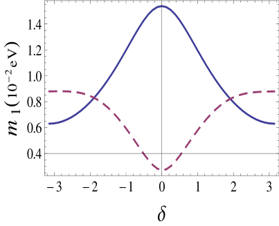
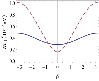
Figure 1: Plots of $m_{1}$ as a function of $\delta$ according to eq. (42) (solid blue line) and eq. (43) (dashed violet line). The points of intersection represent pairs of possible solutions for $(m_{\nu_{1}},\delta)$. Left panel $(+|\theta_{12}|,-|\theta_{23}|)$, right panel $(-|\theta_{12}|,-|\theta_{23}|)$, with $(|\theta_{12}|,|\theta_{23}|)=(34.4^{\circ},42.8^{\circ})$.

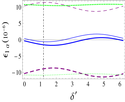
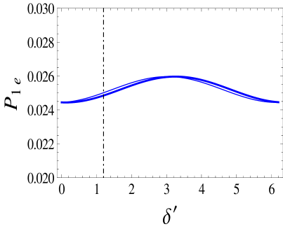
Figure 2: Left: the $N_{1}$ CP asymmetries $\epsilon_{1e}$ (solid blue lines) $\epsilon_{1\mu}$ (dashed violet lines) $\epsilon_{1\tau}$ (dotted green lines) for the solution labeled $(-,-)$ in Table 2 (Case 1) for positive (thick lines) and negative (thin lines) values of the Dirac phase $\delta$, as a function of the $V_{L}$ phase $\delta^{\prime}$. Right: the $N_{1}$ electron flavour washout projector $P_{1e}$ for positive (thick line) and negative (thin line) values of $\delta$ as a function of $\delta^{\prime}$. The vertical dot-dashed lines correspond to the value $\delta^{\prime}=\delta_{CKM}=1.20\,$rad used in the numerical analysis.

The input parameters of our numerical analysis are listed in Table 1. For the eigenvalues of $m_{D}$ we use the values of the up-quark masses renormalized to the scale $\Lambda=10^{9}$ GeV ($\sim M_{R}$), given in Table IV in Ref. Xing:2007fb . The relevant values of $M_{R}$ we find are given in Table 2. Neutrinos mass square differences are taken from the global fit in Ref. GonzalezGarcia:2010er and renormalized to the scale $\Lambda$ with a multiplicative factor $r^{2}$ with $r=1.25$ according to the prescription in Ref. thermal . The CKM mixing angles $\theta^{\prime}_{ij}$ and CKM phase $\delta^{\prime}$ are derived from the values of the Wolfenstein parameters given in Ref. PDG10 , renormalization effects for these angles are small and have been neglected.

As regards the PMNS mixing angles, recent fits to oscillation neutrino data suggest a small but nonvanishing value for $\theta_{13}$. In our scenario, having $\theta_{13}\neq 0$ is of fundamental importance because only under this condition the Dirac phase $\delta$ will enter the constraining equations eq. (40) and eq. (41), providing enough free parameters to allow for a numerical solution, so let us discuss this specific quantity a bit more in detail. With the assumption of normal ordering $m_{1}<m_{2}<m_{3}$, and with $3\sigma$ errors for the three-flavour neutrino oscillation parameters, the following results have been reported:

$$\sin^{2}\theta_{13}=0.013^{+0.023}_{-0.015}\text{\cite[cite]{\@@bibref{Authors Phrase1YearPhrase2}{Schwetz:2011zk}{\@@citephrase{(}}{\@@citephrase{)}}}},\qquad\sin^{2}\theta_{13}=0.025^{+0.025}_{-0.02}\text{\cite[cite]{\@@bibref{Authors Phrase1YearPhrase2}{Fogli:2011qn}{\@@citephrase{(}}{\@@citephrase{)}}}},\qquad\sin^{2}\theta_{13}\leq 0.043\text{\cite[cite]{\@@bibref{Authors Phrase1YearPhrase2}{GonzalezGarcia:2010er}{\@@citephrase{(}}{\@@citephrase{)}}}}\,.$$ (46)

The last result is a 3$\sigma$ upper limit estimated in the framework of the so called GS98 solar model with the Ga capture cross-section of Ref. Bahcall:1997eg . At 1$\sigma$ the same data give $\sin^{2}\theta_{13}=0.0095^{+0.013}_{-0.007}$ corresponding to $\theta_{13}=(5.6^{+3.0}_{-2.7})^{\circ}$ GonzalezGarcia:2010er . We use such best fit value, and also for the other two angles we adopt the results of the global fit in Ref. GonzalezGarcia:2010er .

Our results for the possible values of the still unmeasured low energy parameters $m_{1},\,\delta,\,\alpha$ and $\beta$, and for the RH neutrino masses evaluated according to eq. (15), are collected in Table 2 and in Table 3. Here onwards we always arrange the ordering of RH neutrino masses according to $M_{1}<M_{2}<M_{3}$. The first four lines of Table 2 list the 4+4 possible solutions for the conditions of Case 1 $A_{23}=A_{33}=0$. In each line we list the two solutions corresponding to positive and negative values of $\delta$. Note that the numerical differences between the absolute values of each pair of solutions for $\delta$ are small, since they correspond to effects suppressed by $s_{13}^{\prime}$. However, even such a small difference can have a non negligible impact on the value of the leptogenesis CP asymmetries. Real parameters like $m_{1}$ and $M_{i}$ also come in pairs with very close values, but in this case the differences are numerically irrelevant so that a single approximate value is displayed. This situation is illustrated in Fig. 2: the left panel depicts the three $N_{1}$ flavoured CP asymmetries (see the next section) $\epsilon_{1e}$ (solid blue lines) $\epsilon_{1\mu}$ (dashed violet lines) $\epsilon_{1\tau}$ (dotted green lines) for the solution labeled $(-,-)$ in Table 2 (Case 1) for positive (thick lines) and negative (thin lines) values of the Dirac phase $\delta$, as a function of the $V_{L}$ phase $\delta^{\prime}$. We see that for the CP asymmetries which are very sensitive to the values of the complex phases, the two different solutions for $\delta$ induce very large effects, for example they swap completely the signs of $\epsilon_{1\mu}$ and $\epsilon_{1\tau}$. In the right panel, as an example of one important real leptogenesis parameter, we have plotted the electron flavour washout projector $P_{1e}$ for the RH neutrino $N_{1}$ (see next section), for positive (thick line) and negative (thin line) values of $\delta$ as a function of $\delta^{\prime}$. We see that in this case numerical differences are irrelevant. In both panels the vertical lines correspond to the value $\delta^{\prime}=\delta_{CKM}=1.20\,$rad that we have used in the numerical analysis of Tables 2-3.

The last line in Table 2 labeled with $(-,-)^{*}$ gives the results obtained for that case when $A_{23},\,A_{33}$ are set to small but nonvanishing values, that we have (arbitrarily) chosen as (cfr. eq. (21)):

$$\left|\frac{A_{33}}{A_{22}}\right|=0.05\times\frac{m_{D2}^{2}}{m^{2}_{D3}}\qquad\qquad{\rm and}\qquad\qquad\left|\frac{A_{23}}{A_{22}}\right|=0.05\times\frac{m_{D2}}{m_{D3}}\,.$$ (47)

We see that the changes in $\delta,\,m_{1},\,\alpha$ and $\beta$ with respect to the $A_{23}=A_{33}=0$ case in the fourth line remain below the precision of the table, and in any case are way too small to be seen experimentally. The same happens for all the other cases, and we can thus conclude that the predictions obtained with our simplified conditions eq. (23) hold for each class of compact spectrum solutions. The last column of this line however, makes apparent that the resulting RH spectrum is just compact rather than degenerate, which justifies talking about a third way to SO(10) leptogenesis.

$\left(\theta_{12},\theta_{23}\right)$	$\delta$	$m_{1}\,$($10^{-3}$ eV)	$\alpha$	$\beta$	$(M_{1},\,M_{2},\,M_{3})\,$ ($10^{9}\,$GeV)
$(+,+)$	$(1.43,-1.46)$	$9.7$	$(-1.47,1.46)$	$(-0.18,0.19)$	$(3.5,\ 3.9,\ 3.9)$
$(-,+)$	$(2.60,-2.63)$	$2.9$	$(1.52,-1.51)$	$(1.25,-1.22)$	$(3.0,\ 8.7,\ 8.7)$
$(+,-)$	$(1.91,-1.89)$	$8.2$	$(1.46,-1.44)$	$(0.13,-0.14)$	$(4.0,\ 4.0,\ 4.3)$
$(-,-)$	$(0.74,-0.71)$	$3.1$	$(-1.49,1.48)$	$(-1.19,1.17)$	$(3.5,\ 7.9,\ 7.9)$
$(-,-)^{*}$	$(0.74,-0.71)$	$3.1$	$(-1.49,1.48)$	$(-1.19,1.17)$	$(3.5,\ 7.8,\ 8.0)$

Table 2: The eight possible solutions to the RH neutrino compact spectrum conditions of Case 1: $A_{23}=A_{33}=0$. The real parameters $m_{1}$ and $M_{i}$ also come in pairs as the complex phases $\delta,\,\alpha$ and $\beta$. A single approximate value is displayed because the difference between the two values is numerically irrelevant. For the $(+,-)$ solution, the almost degenerate RH neutrinos are the lighter ones, while in all the other cases are the heavier ones. In the last line, labeled with an asterisk $(-,-)^{*}$, we give the results for the $(-,-)$ solution in which $A_{23}$ and $A_{33}$ are set to arbitrary small, but nonvanishing values (see text).

The conditions $A_{23}=A_{22}=0$ of Case 2 have only 2+2 solutions, that are listed in Table 3. In this case there is a very large hierarchy ${\cal O}(10^{7})$ between the two almost degenerate RH neutrino masses $M_{1,2}$ and $M_{3}$ so that, as expected, the RH spectrum is not compact. Perturbativity of the Yukawa couplings then implies $\Lambda_{R}\mbox{${~{}\raise 2.5pt\hbox{$>$}\kern-6.99997pt\lower 2.5pt\hbox{$\sim$}~{}}$}10^{14}\,$GeV. Accommodating such a large intermediate scale might be problematic in the SO(10) model. Furthermore, as we will see in the next section, in this case leptogenesis is unsuccessful for both the $(-,+)$ and $(-,-)$ solutions.

To conclude this section, we have seen that by forcing the SO(10) model to produce a compact RH neutrino spectrum we obtain a scenario in which all the parameters relevant for leptogenesis remain determined in terms of the set of low energy observables that have been already measured. Most remarkably, as we will see, besides predicting values for the absolute neutrino mass scale $m_{1}$, the CP violating phases, and the RH neutrino spectrum, the size and the signs of the flavoured CP asymmetries relevant for leptogenesis are also fixed, and allow to predict the size and sign of the cosmological baryon asymmetry generated through leptogenesis. Such a level of predictability is indeed quite unusual in see-saw inspired scenarios. Clearly, verifying if the baryon asymmetry yield of leptogenesis is in agreement with observations will now represent the major test of our scenario. This is the task that we are going to address in the next section.

$\left(\theta_{12},\theta_{23}\right)$	$\delta$	$m_{1}\,$($10^{-3}\,$eV)	$\alpha$	$\beta$	$M_{1,2}\,$($10^{7}\,$GeV)	$M_{3}\,$($10^{14}\,$GeV)
$(-,+)$	$(2.66,-2.69)$	$2.0$	$(-1.51,1.52)$	$(-0.21,0.23)$	$3.1$	$3.6$
$(-,-)$	$(0.35,-0.32)$	$2.0$	$(1.53,-1.54)$	$(0.19,-0.21)$	$3.3$	$3.0$

Table 3: Same than Table 2, for the four possible solutions to the conditions of Case 2: $A_{23}=A_{22}=0$.

V Leptogenesis

In the basis for the Dirac mass matrix as in eq. (29), the CP asymmetry in the decay of the RH neutrino $N_{i}$ ($i=1,2,3$) to a lepton $\ell_{\alpha}$ ($\alpha=e,\mu,\tau$) is given by Covi:1996wh

$$\epsilon_{i\alpha} = \frac{1}{8\pi v^{2}}\sum_{k\neq i}\frac{{\rm Im}\left[\left(\hat{m}_{D}^{\dagger}\right)_{i\alpha}\left(\hat{m}_{D}\right)_{\alpha k}\left(\hat{m}_{D}^{\dagger}\hat{m}_{D}\right)_{ik}\right]}{\left(\hat{m}_{D}^{\dagger}\hat{m}_{D}\right)_{ii}}f\left(\frac{M_{k}^{2}}{M_{i}^{2}}\right)$$ (48)

$$+ \frac{1}{8\pi v^{2}}\sum_{k\neq i}\frac{{\rm Im}\left[\left(\hat{m}_{D}^{\dagger}\right)_{i\alpha}\left(\hat{m}_{D}\right)_{\alpha k}\left(\hat{m}_{D}^{\dagger}\hat{m}_{D}\right)_{ki}\right]}{\left(\hat{m}_{D}^{\dagger}\hat{m}_{D}\right)_{ii}}g\left(\frac{M_{k}^{2}}{M_{i}^{2}}\right),$$

where $v=174$ GeV is the EW vev and

$$f(x) = \sqrt{x}\left[\frac{1-x}{\left(1-x\right)^{2}+\left(\frac{\Gamma_{i}}{M_{i}}-x\frac{\Gamma_{k}}{M_{k}}\right)^{2}}+1-\left(1+x\right)\log\frac{1+x}{x}\right],$$

$$g(x) = \frac{1-x}{\left(1-x\right)^{2}+\left(\frac{\Gamma_{i}}{M_{i}}-x\frac{\Gamma_{k}}{M_{k}}\right)^{2}},$$ (49)

are loop functions with $\Gamma_{i}\equiv\frac{M_{i}}{8\pi v^{2}}(\hat{m}_{D}^{\dagger}\hat{m}_{D})_{ii}$ the total $N_{i}$ width. The expression in the second line of eq. (48) corresponds to the lepton-flavour-violating but lepton-number-conserving self-energy diagram. It vanishes when summed over $\alpha$ so it does not contribute in the one-flavour approximation, but plays an important role Nardi:2006fx when, as in our case, leptogenesis occurs in the flavoured regime. In eqs. (49), $g(x)$ and the first term in the square bracket of $f(x)$ come from the self-energy contributions with the resonant condition given by

$$1-x = \pm\left(\frac{\Gamma_{i}}{M_{i}}-x\frac{\Gamma_{k}}{M_{k}}\right),$$ (50)

while the remaining terms in $f(x)$ correspond to contributions from the vertex diagram. The resonant condition eq. (50) gives

$$f(x) \simeq \sqrt{x}g(x)=\frac{\sqrt{x}}{2\left(\frac{\Gamma_{i}}{M_{i}}-x\frac{\Gamma_{k}}{M_{k}}\right)},$$ (51)

where in $f(x)$ we have ignored the subleading contributions of the vertex diagram. However, in our case although the degeneracy conditions $M_{2}\sim M_{3}$ or $M_{1}\sim M_{2}$ are approximately fulfilled, we never reach a fully resonant regime as defined by eq. (50), and hence ignoring the “regulator” term $\left(\frac{\Gamma_{i}}{M_{i}}-x\frac{\Gamma_{k}}{M_{k}}\right)$ in eqs. (49) only yields negligible numerical differences.

In order to calculate the baryon asymmetry, we need to solve a set of Boltzmann equations (BE) (we refer to leptoreview and references therein for details). By including for simplicity only decays and inverse decays, the BE for the RH neutrino densities $Y_{N_{i}}$ and for $Y_{\Delta_{\alpha}}$, that is the asymmetry density of the charge $B/3-L_{\alpha}$ normalized to the entropy density $s$, can be written as:

$$sHz\frac{dY_{N_{i}}}{dz} = -\gamma_{N_{i}}\left(\frac{Y_{N_{i}}}{Y_{N}^{eq}}-1\right),$$

$$sHz\frac{dY_{\Delta_{\alpha}}}{dz} = -\sum_{i}\left[\epsilon_{i\alpha}\gamma_{N_{i}}\left(\frac{Y_{N_{i}}}{Y_{N}^{eq}}-1\right)-\frac{\gamma_{N_{i\alpha}}}{2}\left(\frac{Y_{\Delta\ell_{\alpha}}}{Y_{\ell}^{eq}}+\frac{Y_{\Delta H}}{Y_{H}^{eq}}\right)\right],$$ (52)

where $Y_{N}^{eq}=\frac{45}{4\pi^{4}g_{*}}z^{2}{\cal K}_{2}(z)$ is the equilibrium density for the RH neutrinos with $g_{*}=106.75$ and ${\cal K}_{2}$ the second order modified Bessel function of the second kind, $2Y_{\ell}^{eq}=Y_{H}^{eq}=\frac{15}{4\pi^{2}g_{*}}$ are respectively the equilibrium densities for lepton doublets and for the Higgs, and the integration variable is $z=M/T$ with $T$ the temperature of the thermal bath, and $M=M_{1,2,3}$ the mass of the decaying neutrino. In the above, we have defined $Y_{\Delta_{\alpha}}=Y_{\Delta B}/3-Y_{\Delta L_{\alpha}}$ with $Y_{\Delta L_{\alpha}}$ the total lepton density asymmetry in the $\alpha$ flavour which also includes the asymmetries in the RH lepton singlets. Since RH neutrinos only interact with lepton doublets, the RHS of the second equation of eqs. (52) involves only the LH lepton doublets density asymmetry in a given flavour $\alpha$, $Y_{\Delta\ell_{\alpha}}=A_{\alpha\beta}Y_{\Delta_{\alpha}}$ with $A_{\alpha\beta}$ the flavour mixing matrix flavour0 given in eq. (59) below. In the same equation, we also define $Y_{\Delta H}=C_{\beta}Y_{\Delta_{\beta}}$ the Higgs density asymmetry with $C_{\beta}$ spectator2 also given in eq. (59) and $\gamma_{N_{i\alpha}}=P_{i\alpha}\gamma_{N_{i}}$ (no sum over $i$) where $P_{i\alpha}$ projects the decay rate over the $\alpha$ flavour, that is, it corresponds to the branching ratio for $N_{i}$ decaying to $\ell_{\alpha}$, and can be written as

$$P_{i\alpha}=\frac{\left(\hat{m}_{D}^{\dagger}\right)_{i\alpha}\left(\hat{m}_{D}\right)_{\alpha i}}{\left(\hat{m}_{D}^{\dagger}\hat{m}_{D}\right)_{ii}}.$$ (53)

Let us also introduce the rescaled decay width

$${\widetilde{m}}_{i}\equiv\frac{8\pi{v^{2}}}{M_{i}^{2}}\Gamma{{}_{i}}=\frac{(\hat{m}_{D}^{\dagger}\hat{m}_{D})_{ii}}{M_{i}},$$ (54)

which is also known as the effective washout parameter, that parametrizes conveniently the departure from thermal equilibrium of $N_{i}$-related processes (the larger ${\widetilde{m}}_{i}$, the closer to thermal equilibrium the decays and inverse decays of $N_{i}$ occur, thus suppressing the final lepton asymmetry). Finally, the combination $P_{i\alpha}\,{\widetilde{m}}_{i}$ projects the washout parameter over a particular flavour direction, and determines how strongly the lepton asymmetry of flavour $\alpha$ is washed out.

Leptogenesis becomes possible when the thermal bath temperature approaches the value of the mass of the decaying RH neutrino, that becomes non relativistic and can decay. However, when the washout parameter is large $\widetilde{m}\mbox{${~{}\raise 2.5pt\hbox{$>$}\kern-6.99997pt\lower 2.5pt\hbox{$\sim$}~{}}$}10^{-3}$, at $T\sim M_{i}$ the RH neutrinos are actually in equilibrium and no asymmetry can be generated. In our case the RH neutrinos are coupled rather strongly to the thermal bath ($\widetilde{m}\gg 10^{-3}$ see e.g. Table 4) and in this case the generation of the bulk of the lepton asymmetry is delayed down to much lower temperatures: for $\widetilde{m}\sim 6\times 10^{-2}$ for example one can estimate $z=M/T\sim 8$ Buchmuller:2004nz ). Thus, the range of temperatures where the lepton asymmetry is generated falls well below $10^{9}\,{\rm GeV}$, where both the $\tau$ and $\mu$ Yukawa interactions are presumably in equilibrium leptoreview . In this regime all the three lepton flavours are then distinguished, and their dynamical evolution must be followed separately. The $A$ flavour mixing matrix and the $C$ vectors allow to accomplish this task, and in our temperature regime are given by Nardi:2006fx

$$A = \frac{1}{2148}\left(\begin{array}[]{ccc}-906&120&120\\ 75&-688&28\\ 75&28&-688\end{array}\right),$$ (58)

$$C = -\frac{1}{358}\left(37,52,52\right).$$ (59)

Once the final asymmetries in the lepton flavour charge densities $Y_{\Delta_{\alpha}}$ are obtained by solving numerically the BE eq. (52), the baryon asymmetry generated through leptogenesis is given by Harvey:1990qw

$$Y_{\Delta B} = \frac{28}{79}\sum_{\alpha}Y_{\Delta_{\alpha}}\,.$$ (60)

The resulting prediction should then be confronted with the experimental number. The most precise experimental determination of $Y_{\Delta B}$ is obtained from measurements of the cosmic microwave background (CMB) anisotropies. A fit to the most recent observations (WMAP7 data only, assuming a $\Lambda$CDM model with a scale-free power spectrum for the primordial density fluctuations) Larson:2010gs , when translated in terms of $Y_{\Delta B}$ gives at 95% c.l. Fong:2011yx

$$Y_{\Delta B}^{CMB}=(8.79\pm 0.44)\times 10^{-11}.$$ (61)

V.1 Numerical Results

For all the phenomenologically viable cases stemming out from our scenario, the complete set of high energy parameters required for computing the baryon asymmetry yield of leptogenesis is predicted. The RH neutrino masses are listed for Case 1 in the last column in Table 2, and for Case 2 in the last column of Table 3 (of course, the precise numerical values of the masses, rather then the approximate values listed in the tables, are used for the leptogenesis computation). As regards the flavoured CP asymmetries, they are computed according to eq. (48) and the corresponding results for our two cases are listed in Table 4 and 5. Case 1 (Table 4) results in a very compact spectrum of RH neutrinos (and with a pair of almost degenerate states if the exact conditions $A_{23}=A_{33}=0$ are imposed). For solutions $(+,+)$ and $(+,-)$ the largest mass differences remain at the 10% level, while for solutions $(-,+)$ and $(-,-)$ they reach a factor of a few. Under this conditions it is mandatory to include the contributions from the heavier RH neutrinos, that in the first case (of tiny mass differences) can affect the results for a factor up to ${\cal O}(10^{3})$. For Case 1 (Table 4), that contains sub-cases in which leptogenesis can be successful, we give the complete list of the $N_{1}$ flavoured parameters: the CP asymmetries for the three flavours are given in columns 2-4, the washout flavour projectors in columns 5-7, and the effective washout parameters in column 8. The final results obtained by integrating the BE and by converting $Y_{\Delta_{B-L}}=\sum_{\alpha}Y_{\Delta_{\alpha}}$ into $Y_{\Delta_{B}}$ through eq. (60) are given in the last column of the two tables. Columns 2-4 in Table 4 show that asymmetries of different signs are produced in different lepton flavours (an example of this situation is also depicted in the left panel in Fig. 2), while columns 5-7 show that a certain hierarchy exists between the flavoured washout parameters. Given the highly non uniform pattern in flavour space of the relevant leptogenesis quantities it is clear that no analytical expression based on the single flavour approximation would produce a reliable result, and we can firmly conclude that lepton flavour dynamics is of crucial importance for studying leptogenesis in the SO(10) model.

$\left(\theta_{12},\theta_{23}\right)$	$\epsilon_{1e}\,$$(10^{-5})$	$\epsilon_{1\mu}\,$$(10^{-5})$	$\epsilon_{1\tau}\,$$(10^{-5})$	$P_{1e}$	$P_{1\mu}$	$P_{1\tau}$	$\widetilde{m}_{1}$($10^{-2}$ eV)	$Y_{\Delta B}$$(10^{-10})$
$(+,+)$	$(0.9,0.5)$	$(3.4,-5.0)$	$(-4.3,4.5)$	$10^{-3}$	$0.03$	$0.97$	$74$	$(-0.3,-0.08)$
$(-,+)$	$(0.041,0.083)$	$(-0.52,0.41)$	$(0.47,-0.49)$	$0.03$	$0.50$	$0.47$	$6.2$	$(-0.8,-1.5)$
$(+,-)$	$(-0.001,-0.001)$	$(0.003,-0.001)$	$(-2.5,2.6)$	$10^{-4}$	$10^{-3}$	$1.0$	$10^{5}$	$(0.03,0.07)$
$(-,-)$	$(-0.16,-0.06)$	$(-0.89,1.14)$	$(1.05,-1.09)$	$0.03$	$0.47$	$0.50$	$6.7$	$(2.3,0.32)$
$(-,-)^{*}$	$(-0.05,-0.04)$	$(-0.05,0.15)$	$(-0.15,0.15)$	$10^{-3}$	$0.06$	$0.94$	$70$	$(0.43,0.38)$

Table 4: The leptogenesis parameters corresponding to the different solutions of Case 1.

For Case 2, given that all the solutions consistent with the low energy constraints eventually fail the leptogenesis test, we just give in Table 5 the total CP asymmetries and the approximate values of the total washout parameters for the two quasi degenerate RH neutrinos $N_{1,2}$. This reduced set of figures is however sufficient to conclude at a first glance that with CP asymmetries of ${\cal O}(10^{-8})$ and washout parameters of ${\cal O}(1\,$eV), no flavour dynamics could rescue leptogenesis from a quantitative failure.

Our results are collected in the last columns of Tables 4 and Table 5. Although we are using somewhat simplified BE in which thermal corrections thermal , scatterings and CP violation in scatterings flavour3 ; Nardi:2007jp ; Fong:2010bh , and other subleading effects are neglected, the estimates of the final baryon asymmetry we obtain should be sufficiently accurate for our scopes. For example, we have checked that including scatterings and CP violations in scatterings introduces a $\lesssim~{}$25 % effect, which is by no means crucial to test the scenario. There are in fact other important sources of uncertainties: in our analysis we are using fixed central vales for all the input parameters, and it goes without saying that the final value of $Y_{\Delta B}$ will be affected by the experimental uncertainties. Even more importantly, there are also theoretical uncertainties stemming from deviations from the exact quark-lepton symmetry ansatz eq. (9), as well as from deviations from the exact zeroes in the conditions $A_{23}=A_{33}=0$, which are obviously difficult to quantify. Therefore, we will be contented to require that a successful prediction of the BAU, besides having the correct sign, should approach the experimental result eq. (61) only within a factor of a few. For Case 1, we obtain four solutions with the wrong (negative) sign of the BAU, and other four with the correct sign. They are listed in Table 4. However, only the two solutions in the fourth line of the Table are sufficiently close to the experimental value eq. (61) to be all phenomenologically acceptable. For this two solutions we give in the last line of the Table the values of the leptogenesis parameters for $N_{1}$, and of the final baryon asymmetry when the exact zeroes in eq. (23) are lifted to small but not vanishing values as given in eq. (47). We see that although the final value of $Y_{\Delta B}$ is sensitive to this change, it still remains within a factor of two from the measured central value eq. (61).

As we have already said, in this SO(10) scenario the leptogenesis efficiency gets largely enhanced by flavour effects, and it is then worth asking what would happen if the bulk of the lepton asymmetry, rather than in the three flavour regime, is generated when only the $\tau$ Yukawa coupling mediated in-equilibrium reactions, and the number of relevant flavour is reduced to two. In the two flavour and strong washout case, estimating $Y_{\Delta B}$ is more subtle because there can be protected directions in which the asymmetry generated by $N_{2,3}$ is not erased by $N_{1}$ washouts N2 ; Antusch:2010ms . We follow a simplified approach that neglects this phenomena, and thus gives a conservative estimate of the final asymmetry, obtaining for the $(-,-)$ case $Y_{\Delta B}\mbox{${~{}\raise 2.5pt\hbox{$>$}\kern-6.99997pt\lower 2.5pt\hbox{$\sim$}~{}}$}(0.3,-0.3)\times 10^{-10}$. In the first case the asymmetry gets reduced, but still remains within a factor of three from the experimental number; however, in the second case the asymmetry changes sign, which again shows the importance of a proper treatment of flavour dynamics.

As regards Case 2, we see that the two right-sign solutions yield a baryon asymmetry that is too small by almost three order of magnitudes. This suppression of $Y_{\Delta B}$ is due to two different reasons: firstly the CP asymmetries are exceedingly small because the imaginary parts of the relevant combinations of couplings are strongly suppressed, and secondly the washout parameters are rather large, and imply an almost in-equilibrium dynamics that impedes building up any sizable density asymmetries.

In conclusion, the SO(10) model constrained by the assumption of the quark-lepton symmetry in eq. (9) and by the compact RH neutrino spectrum conditions in eq. (23), when confronted with the results from neutrino oscillation experiments, and with the requirement of successful leptogenesis, yields predictions for the yet unknown low energy neutrino parameters, that are summarized in the following two possibilities

$$(--):\qquad m_{\nu_{1}}\simeq 3\times 10^{-3}\,{\rm eV},\qquad\delta\simeq\,\pm\,0.7\,,\qquad\alpha\simeq\,\mp 1.5\,,\qquad\beta\simeq\,\mp 1.2\,,$$ (62)

which correspond to either the upper or lower sign of the three phases.

With the numerical results listed in eq. (62) another low energy observable can be predicted, that is the neutrinoless double beta decay effective parameter

$$m_{ee}\equiv(m_{\nu})_{11}=\sum_{i}({U_{PMNS}^{\star}})_{1i}{(m_{\nu})_{i}^{diag}}({U_{PMNS}^{\dagger}})_{i1}\,,$$ (63)

for which we obtain $|m_{ee}|\mbox{${~{}\raise 2.5pt\hbox{$<$}\kern-6.99997pt\lower 2.5pt\hbox{$\sim$}~{}}$}2\>\times 10^{-3}\,$eV that, as could have been expected for hierarchical and normal ordered neutrino masses, remains well below the sensitivity of all ongoing and planned experiments Barabash:2011fg .

$\left(\theta_{12},\theta_{23}\right)$	$\epsilon_{1}\,$$(10^{-8})$	$\epsilon_{2}\,$$(10^{-8})$	$\widetilde{m}_{1,2}\,$(eV)	$Y_{\Delta B}\,$$(10^{-14})$
$(-,+)$	$(5.4,-5.5)$	$(5.4,-5.5)$	$1.7$	$(-1.8,1.8)$
$(-,-)$	$(-4.3,5.0)$	$(-4.3,5.0)$	$1.6$	$(1.5,-1.7)$

Table 5: The leptogenesis parameters corresponding to the different solutions of Case 2.

VI Discussion and Conclusions

The predictive power of our scenario is spelled out in clear in eq. (62), and such a high level of predictability calls for an explanation. The crucial point is that in our study there are no free parameters: everything is fixed in terms of the low energy neutrino observables and by the additional assumption of quark-lepton symmetry eq. (9) and by the compact RH spectrum conditions $A_{23}=A_{33}=0$. The only freedom left over by these latter constraints is a discrete one, and corresponds to the signs of the two angles $\theta_{12}$ and $\theta_{23}$, for each choice of which there are in turn two solutions, corresponding to positive and negative values of the phase $\delta$. Given that there is no free parameter that can be adapted to fit the observed value of the BAU, we find intriguing that among the discrete set of eight possibilities of Case 1, in two cases the leptogenesis yield of baryon asymmetry is in acceptable agreement with observations.

To summarize the main results of the paper, we have first shown that in the SO(10) seesaw model it is technically possible to arrange for a compact RH neutrino spectrum, and this in spite of the fact that the SO(10) neutrino Dirac mass matrix is characterized by a hierarchy between its eigenvalues that is much stronger than the one observed for the the light neutrinos, a situation that would naturally call for a compensating large hierarchy in the RH masses. We have argued that this possibility can be implemented in a consistent way only if the PMNS mixing angle $\theta_{13}$ is nonvanishing, since only in this case we have at disposal the Dirac phase $\delta$ as an additional free physical parameter that can cope with satisfying the compact RH spectrum conditions. The counting of free parameters is a subtle point: clearly our construction relies quantitatively on the assumption of a strict quark-lepton symmetry $m_{D}=m_{u}$ and $V_{L}=V_{CKM}$, and one might argue that even in the absence of $\delta$ one could be able to find solutions by modifying these assumptions. Nevertheless, in SO(10) $m_{D}$ and $V_{L}$ are intrinsically related to $m_{u}$ and $V_{CKM}$, simply by the fact that all fermions of each family, including the RH neutrino, are assigned to the same irreducible representation of the group. The important point is that while the precise form of the quark-lepton duality relations can be changed according to the amount of (family dependent) contamination in the EW breaking sector from $\mathbf{10}$ and $\mathbf{126}$ vevs, still $m_{D}$ and $V_{L}$ cannot be regarded as independent from the corresponding quantities in quark sector, since for any fixed pattern of vevs, some specific relation between them remains fixed. Therefore, the compact spectrum conditions together with any specific assumption about lepton-quark Yukawa relations, always yields a scenario where the values of the yet unknown neutrino parameters can be predicted directly in terms of known quantities. This is not so for the absolute neutrino mass scale $m_{1}$ which is a true free parameter, since it is essentially determined by the ratio $\Lambda_{EW}/\Lambda_{R}$ where the scale $\Lambda_{R}$ is free, nor for the PMNS phase $\delta$ since the complex phases in $M_{R}$, that are unrelated to $V_{CKM}$ and thus are also free, concur to determine its value.

As regards the compact RH spectrum conditions $A_{23}=A_{33}=0$ eq. (23), they should be understood with a grain of salt. Rather than corresponding to exact zeroes, the assumption is that to a good approximation the values of these entries are negligible. This is spelled out in eq. (21) and eq. (22). We have also tested the effects of lifting the exact zeros to the small nonvanishing values given in eq. (47) finding that (i) the quasi degeneracy in the RH neutrino mass eigenvalues is removed, resulting in a generic compact spectrum; (ii) the predictions for the measurable low energy parameters (the absolute neutrino mass scale and the CP violating phases) are not changed; (iii) the effects on the final value of $Y_{\Delta B}$ remain under control. We stress again that we have not put forth any theoretical explanation, as for example a symmetry argument, for why the entries $A_{23}$ and $A_{33}$ should be particularly suppressed, and this implies that the fact that the four (real plus imaginary) conditions can be fulfilled only if specific quantitative relations between $m_{1},\,\delta,\,\alpha$ and $\beta$ are satisfied, should not be confused with a parametric (i.e. functional) dependence like $\delta=\delta(m_{1})$ or $\alpha=\alpha(m_{1},\delta)$, which is something that our SO(10) scenario certainly does not give, but should rather be regarded as numerical accidents.

It is likely that in the not too far future the values of $m_{1}$ and of $\delta$ will eventually be measured, and therefore the specific scenario we have been exploring, and whose predictions are summarized in eq. (62), is straightforwardly falsifiable. Of course, by modifying the form of the quark-lepton symmetry relations one would obtain numerically different predictions. However, any different assumption would result in the same level of predictability, and in particular it will have to pass the leptogenesis test which, as we have seen, is a highly nontrivial requirement. It is certainly conceivable a situation in which no assumption will be able to reproduce the measured values of $m_{1}$ and $\delta$ while simultaneously pass the leptogenesis test. We can then conclude that the leptogenesis scenario based on SO(10) with a compact RH neutrino spectrum is a testable physical hypothesis.

Note added

After this paper was published in the arXiv.org database Buccella:2012kc , the Daya Bay reactor neutrino experiment announced the measurement of a non-zero value for the neutrino mixing angle $\theta_{13}$ with a significance of 5.2 standard deviations: $\sin^{2}2\theta_{13}=0.092\pm 0.016{\rm(stat.)}\pm{\rm 0.005(syst.)}$ An:2012eh . In April 2012, the RENO experiment also reported a non zero value $\sin^{2}2\theta_{13}=0.113\pm 0.013{\rm(stat.)}\pm{\rm 0.019(syst.)}$ Ahn:2012nd consistent with the Day Bay result. As we have explained in the paragraph above eq. (46), $\theta_{13}\neq 0$ is a mandatory condition for the consistency of our scenario, which is now ensured by the Daya Bay and RENO results. The experimental central values $\theta_{13}=8.8^{\circ}$ (Daya Bay) and $\theta_{13}=9.8^{\circ}$ (RENO) are larger than our reference value $\theta_{13}=5.6^{\circ}$ GonzalezGarcia:2010er (see below eq. (46)), and this will slightly change the numbers in eq. (62). However, the conclusions of the leptogenesis analysis that are based on the sign of the baryon asymmetry and on its value only within a factor of a few, will not be changed. To give an example, for $\theta_{13}=8.8^{\circ}$ we obtain for the first of the two cases labeled $(-,-)$ in Table 4 $Y_{\Delta B}=2.9\times 10^{-10}$ instead than $Y_{\Delta B}=2.3\times 10^{-10}$ which clearly implies the same conclusions.

References

- (1) B. Pontecorvo, Sov. Phys. JETP 6 (1957) 429 [Zh. Eksp. Teor. Fiz. 33 (1957) 549]; B. Pontecorvo, Sov. Phys. JETP 7 (1958) 172 [Zh. Eksp. Teor. Fiz. 34 (1957) 247].
- (2) P. Minkowski, Phys. Lett. B67 (1977) 421; M. Gell-Mann, P. Ramond and R. Slansky, in , Eds. P. van Nieuwenhuizen and D. Freedman (North Holland, Amsterdam, 1979); T. Yanagida in United Theories and Baryon Number in the Universe, Eds. O. Sawada and A. Sugamoto (KEK, Tsukuba, 1979); R. N. Mohapatra and G. Senjanovic, Phys. Rev. Lett. 44 (1980) 912.
- (3) H. Georgi, in , ed. C. Carlson (AIP, New York, 1975).
- (4) H. Fritzsch and P. Minkowski, Annals Phys. 93 (1975) 193 .
- (5) M. Fukugita and T. Yanagida, Phys. Lett. B174 (1986) 45.
- (6) S. Davidson, E. Nardi and Y. Nir, Phys. Rept. 466 (2008) 105.
- (7) F. Buccella, D. Falcone and L. Oliver, Phys. Rev. D83 (2011) 093013.
- (8) R. Barbieri et al., Nucl. Phys. B575 (2000) 61; T. Endoh, T. Morozumi and Z. h. Xiong, Prog. Theor. Phys. 111 (2004) 123.
- (9) A. Abada, S. Davidson, F. -X. Josse-Michaux, M. Losada and A. Riotto, JCAP 0604 (2006) 004.
- (10) E. Nardi, Y. Nir, E. Roulet and J. Racker, JHEP 0601 (2006) 164.
- (11) G. Engelhard, Y. Grossman, E. Nardi and Y. Nir, Phys. Rev. Lett. 99, (2007) 081802.
- (12) S. Antusch, P. Di Bari, D. A. Jones and S. F. King, Nucl. Phys. B 856, 180 (2012) [arXiv:1003.5132 [hep-ph]].
- (13) T. Schwetz, M. Tortola and J. W. F. Valle, New J. Phys. 13 (2011) 109401.
- (14) G. L. Fogli, E. Lisi, A. Marrone, A. Palazzo and A. M. Rotunno, Phys. Rev. D84 (2011) 053007.
- (15) M. C. Gonzalez-Garcia, M. Maltoni and J. Salvado, JHEP 1004 (2010) 056.
- (16) Z. Maki, M. Nakagawa and S. Sakata, Prog. Theor. Phys. 28 (1962) 870.
- (17) S. M. Bilenky and B. Pontecorvo, Phys. Rept. 41 (1978) 225.
- (18) J. C. Pati and A. Salam, Phys. Rev. D10 (1974) 275.
- (19) H. Georgi and C. Jarlskog, Phys. Lett. B86 (1979) 297.
- (20) J. A. Harvey, P. Ramond and D. B. Reiss, Phys. Lett. B92 (1980) 309.
- (21) J. A. Harvey, D. B. Reiss and P. Ramond, Nucl. Phys. B199 (1982) 223.
- (22) E. K. Akhmedov, M. Frigerio and A. Y. .Smirnov, JHEP 0309 (2003) 021.
- (23) D. Falcone and F. Tramontano, Phys. Rev. D63 (2001) 073007.
- (24) E. Nezri and J. Orloff, JHEP 0304 (2003) 020.
- (25) S. Davidson and A. Ibarra, Phys. Lett. B535 (2002) 25.
- (26) P. Di Bari, Nucl. Phys. B727 (2005) 318.
- (27) O. Vives, Phys. Rev. D73 (2006) 073006.
- (28) A. Abada, P. Hosteins, F. X. Josse-Michaux and S. Lavignac, Nucl. Phys. B809 (2009) 183.
- (29) P. Di Bari and A. Riotto, Phys. Lett. B671 (2009) 462.
- (30) P. Di Bari and A. Riotto, JCAP 1104 (2011) 037.
- (31) S. Blanchet, D. Marfatia and A. Mustafayev, JHEP 1011, 038 (2010).
- (32) A. Pilaftsis and T. E. J. Underwood, Nucl. Phys. B692 (2004) 303; A. Pilaftsis and T. E. J. Underwood, Phys. Rev. D72 (2005) 113001; A. Pilaftsis, Phys. Rev. Lett. 95, (2005) 081602.
- (33) T. Takagi, Japanese J. Math. 1 (1927) 83.
- (34) S. Bertolini, L. Di Luzio and M. Malinsky, Phys. Rev. D 80, 015013 (2009).
- (35) S. Bertolini, L. Di Luzio and M. Malinsky, arXiv:1202.0807 [hep-ph].
- (36) A. Y. Smirnov, Phys. Rev. D48 (1993) 3264.
- (37) Z. z. Xing, H. Zhang and S. Zhou, Phys. Rev. D 77 (2008) 113016
- (38) G. F. Giudice, A. Notari, M. Raidal, A. Riotto and A. Strumia, Nucl. Phys. B685 (2004) 89.
- (39) K. Nakamura et al. (Particle Data Group), J. Phys. G37 (2010) 075021.
- (40) J. N. Bahcall, Phys. Rev. C56 (1997) 3391.
- (41) L. Covi, E. Roulet and F. Vissani, Phys. Lett. B 384 (1996) 169
- (42) A. Anisimov, A. Broncano and M. Plumacher, Nucl. Phys. B737 (2006) 176.
- (43) W. Buchmuller and M. Plumacher, Phys. Lett. B431 (1998) 354.
- (44) E. Nardi, Y. Nir, E. Roulet and J. Racker, JHEP 0601 (2006) 164.
- (45) E. Nardi, Y. Nir, J. Racker and E. Roulet, JHEP 0601 (2006) 068.
- (46) W. Buchmuller, P. Di Bari and M. Plumacher, Annals Phys. 315, 305 (2005) [hep-ph/0401240].
- (47) J. A. Harvey and M. S. Turner, Phys. Rev. D42 (1990) 3344.
- (48) D. Larson et al., Astrophys. J. Suppl. 192 (2011) 16.
- (49) C. S. Fong, M. C. Gonzalez-Garcia and E. Nardi, Int. J. Mod. Phys.A26 3491 (2011).
- (50) A. Abada, S. Davidson, A. Ibarra, F. X. Josse-Michaux, M. Losada and A. Riotto, JHEP 0609 (2006) 010.
- (51) E. Nardi, J. Racker and E. Roulet, JHEP 0709 (2007) 090.
- (52) C. S. Fong, M. C. Gonzalez-Garcia and J. Racker, Phys. Lett. B697 (2011) 463.
- (53) See for example: A. S. Barabash, Phys. Part. Nucl. 42 (2011) 613.
- (54) F. Buccella, D. Falcone, C. S. Fong, E. Nardi and G. Ricciardi, arXiv:1203.0829 [hep-ph].
- (55) F. P. An et al. [DAYA-BAY Collaboration], Phys. Rev. Lett. 108, 171803 (2012) [arXiv:1203.1669 [hep-ex]].
- (56) J. K. Ahn et al. [RENO Collaboration], Phys. Rev. Lett. 108, 191802 (2012) [arXiv:1204.0626 [hep-ex]].