Chernoff’s density is log-concave

Abstract

We show that the density of $Z=\mathop{\operatorname{argmax}}\{W(t)-t^{2}\}$, sometimes known as Chernoff’s density, is log-concave. We conjecture that Chernoff’s density is strongly log-concave or “super-Gaussian”, and provide evidence in support of the conjecture.

and

1 Introduction: Two limit theorems

We begin by comparing two limit theorems.

First the usual central limit theorem: Suppose that $X_{1},\ldots,X_{n}$ are i.i.d. $EX_{1}=\mu$, $E(X^{2})<\infty$, $\sigma^{2}=\operatorname{Var}(X)$. Then, the classical Central Limit theorem says that

$$\sqrt{n}(\overline{X}_{n}-\mu)\rightarrow_{d}N\bigl{(}0,\sigma^{2}\bigr{)}.$$

The Gaussian limit has density

$$\phi_{\sigma}(x) = \frac{1}{\sqrt{2\uppi}\sigma}\exp\biggl{(}-\frac{x^{2}}{2\sigma^{2}}\biggr{)}=\mathrm{e}^{-V(x)},$$

$$V(x) = -\log\phi_{\sigma}(x)=\frac{x^{2}}{2\sigma^{2}}+\log(\sqrt{2\uppi}\sigma),$$

$$V^{\prime\prime}(x) = (-\log\phi_{\sigma})^{\prime\prime}(x)=\frac{1}{\sigma^{2}}>0.$$

Thus, $\log\phi_{\sigma}$ is concave, and hence $\phi_{\sigma}$ is a log-concave density. As is well known, the normal distribution arises as a natural limit in a wide range of settings connected with sums of independent and weakly dependent random variables; see, for example, Le Cam [30] and Dehling and Philipp [11].

Now for a much less well-known limit theorem in the setting of monotone regression. Suppose that the real-valued function $r(x)$ is monotone increasing for $x\in[0,1]$. For $i\in\{1,\ldots,n\}$, suppose that $x_{i}=i/(n+1)$, $\varepsilon_{i}$ are i.i.d. with $E(\varepsilon_{i})=0$, $\sigma^{2}=E(\varepsilon_{i}^{2})<\infty$, and suppose that we observe $(x_{i},Y_{i})$, $i=1,\ldots,n$, where

$$Y_{i}=r(x_{i})+\varepsilon_{i}\equiv\mu_{i}+\varepsilon_{i},\qquad i\in\{1,\ldots,n\}.$$

The isotonic estimator $\widehat{\underline{\mu}}$ of $\underline{\mu}=(\mu_{1},\ldots,\mu_{n})$ is given by

$$\widehat{\mu}_{j} = \max_{i\leq j}\min_{k\geq j}\biggl{\{}\frac{\sum_{l=i}^{k}Y_{l}}{k-i+1}\biggr{\}},$$

$$\widehat{\underline{\mu}} = (\hat{\mu}_{1},\ldots,\hat{\mu}_{n})\equiv T\underline{Y}$$

$$= \mbox{least squares projection of }\underline{Y}\mbox{ onto }K_{n},$$

$$K_{n} = \bigl{\{}y\in\mathbb{R}^{n}\colon\ y_{1}\leq\cdots\leq y_{n}\bigr{\}}.$$

For fixed $x_{0}\in(0,1)$ with $x_{j}\leq x_{0}<x_{j+1}$ we set $\hat{r}_{n}(x_{0})\equiv\hat{r}_{n}(x_{j})=\hat{\mu}_{j}$.

Brunk [7] showed that if $r^{\prime}(x_{0})>0$ and if $r^{\prime}$ is continuous in a neighborhood of $x_{0}$, then

$$n^{1/3}\bigl{(}\widehat{r}_{n}(x_{0})-r(x_{0})\bigr{)}\rightarrow_{d}\bigl{(}\sigma^{2}r^{\prime}(x_{0})/2\bigr{)}^{1/3}(2Z_{1}),$$

where, with $\{W(t)\colon\ t\in\mathbb{R}\}$ denoting a two-sided standard Brownian motion process started at $0$,

$$2Z_{1} = \mbox{slope at zero of the greatest convex minorant of }W(t)+t^{2}$$

$$\stackrel{{\scriptstyle d}}{{=}} \mbox{slope at zero of the least concave majorant of }W(t)-t^{2}$$

$$\stackrel{{\scriptstyle d}}{{=}} 2\operatorname{argmin}\bigl{\{}W(t)+t^{2}\bigr{\}}.$$

The density $f$ of $Z_{1}$ is called Chernoff’s density. Chernoff’s density appears in a number of nonparametric problems involving estimation of a monotone function:

• Estimation of a monotone regression function $r$: see, for example, Ayer et al. [1], van Eeden [44], Brunk [7], and Leurgans [31].

• Estimation of a monotone decreasing density: see Grenander [12], Prakasa Rao [37], and Groeneboom [14].

• Estimation of a monotone hazard function: Grenander [13], Prakasa Rao [38], Huang and Zhang [26], Huang and Wellner [25].

• Estimation of a distribution function with interval censoring: Groeneboom and Wellner [21], Groeneboom [16].

In each case:

• There is a monotone function $m$ to be estimated.

• There is a natural nonparametric estimator $\widehat{m}_{n}$.

• If $m^{\prime}(x_{0})\not=0$ and $m^{\prime}$ continuous at $x_{0}$, then

  $$n^{1/3}\bigl{(}\widehat{m}_{n}(x_{0})-m(x_{0})\bigr{)}\rightarrow_{d}C(m,x_{0})2Z_{1},$$

  where $2Z_{1}$ is as in (1).

See Kim and Pollard [29] for a unified approach to these types of problems.

The first appearance of $Z_{1}$ was in Chernoff [9]. Chernoff [9] considered estimation of the mode of a (symmetric unimodal) density $f$ via the following simple estimator: if $X_{1},\ldots,X_{n}$ are i.i.d. with density $h$ and distribution function $H$, then for each fixed $a>0$ let

$$\hat{x}_{a}\equiv\mbox{center of the interval of length }2a\mbox{ containing the most observations}.$$

Let $x_{a}$ be the center of the interval of length $2a$ maximizing $H(x+a)-H(x-a)=P(X\in(x-a,x+a])$. (Note that this $x_{a}$ is not the mode if $f$ is not symmetric.) Then Chernoff shows:

$$n^{1/3}(\hat{x}_{a}-x_{a})\rightarrow_{d}\biggl{(}\frac{h(x_{a}+a)}{c}\biggr{)}^{1/3}2Z_{1},$$

where $c\equiv h^{\prime}(x_{a}-a)-h^{\prime}(x_{a}+a)$. Chernoff also showed that the density $f_{Z_{1}}=f$ of $Z_{1}$ has the form

$$f(z)\equiv f_{Z_{1}}(z)={\textstyle\frac{1}{2}}g(z)g(-z),$$ (2)

where

$$g(t)\equiv\lim_{x\nearrow t^{2}}\frac{\partial}{\partial x}u(t,x),$$

where, with $W$ standard Brownian motion,

$$u(t,x)\equiv P^{(t,x)}\bigl{(}W(z)>z^{2},\mbox{for some }z\geq t\bigr{)}$$

is a solution to the backward heat equation

$$\frac{\partial}{\partial t}u(t,x)=-\frac{1}{2}\frac{\partial^{2}}{\partial x^{2}}u(t,x)$$

under the boundary conditions

$$u\bigl{(}t,t^{2}\bigr{)}=\lim_{x\nearrow t^{2}}u(t,x)=1,\qquad\lim_{x\rightarrow-\infty}u(t,x)=0.$$

Again let $W(t)$ be standard two-sided Brownian motion starting from zero, and let $c>0$. We now define

$$Z_{c}\equiv\sup\bigl{\{}t\in\mathbb{R}\colon\ W(t)-ct^{2}\mbox{ is maximal}\bigr{\}}.$$ (3)

As noted above, $Z_{c}$ with $c=1$ arises naturally in the limit theory for nonparametric estimation of monotone (decreasing) functions. Groeneboom [15] (see also Daniels and Skyrme [10]) showed that for all $c>0$ the random variable $Z_{c}$ has density

$$f_{Z_{c}}(t)={\textstyle\frac{1}{2}}g_{c}(t)g_{c}(-t),$$

where $g_{c}$ has Fourier transform given by

$$\hat{g}_{c}(\lambda)=\int_{-\infty}^{\infty}\mathrm{e}^{\mathrm{i}\lambda s}g_{c}(s)\,\mathrm{d}s=\frac{2^{1/3}c^{-1/3}}{\operatorname{Ai}(\mathrm{i}(2c^{2})^{-1/3}\lambda)}.$$ (4)

Groeneboom and Wellner [22] gave numerical computations of the density $f_{Z_{1}}$, distribution function, quantiles, and moments.

Recent work on the distribution of the supremum $M_{c}\equiv\sup_{t\in\mathbb{R}}(W(t)-ct^{2})$ is given in Janson, Louchard and Martin-Löf [27] and Groeneboom [17]. Groeneboom [18] studies the number of vertices of the greatest convex minorant of $W(t)+t^{2}$ in intervals $[a,b]$ with $b-a\rightarrow\infty$; the function $g_{c}$ with $c=1$ also plays a key role there.

Our goal in this paper is to show that the density $f_{Z_{c}}$ is log-concave. We also present evidence in support of the conjecture that $f_{Z_{c}}$ is strongly log-concave: that is, $(-\log f_{Z_{c}})^{\prime\prime}(t)\geq\mbox{some }c>0$ for all $t\in\mathbb{R}$.

The organization of the rest of the paper is as follows: log-concavity of $f_{Z_{c}}$ is proved in Section 2 where we also give graphical support for this property and present several corollaries and related results. In Section 3, we give some partial results and further graphical evidence for strong log-concavity of $f\equiv f_{Z_{1}}$: that is,

$$(-\log f)^{\prime\prime}(t)\geq(-\log f)^{\prime\prime}(0)=3.4052\ldots=1/(0.541912\ldots)^{2}\equiv 1/\sigma_{0}^{2}\vspace*{-1pt}$$

for all $t\in\mathbb{R}$. As will be shown in Section 3, this is equivalent to $f(t)=\rho(t)\phi_{\sigma_{0}}(t)$ with $\rho$ log-concave. In Section 4, we briefly discuss some of the consequences and corollaries of log-concavity and strong log-concavity, sketch connections to some results of Bondesson [5, 6], and list a few of the many further problems.

2 Chernoff’s density is log-concave

Recall that a function $h$ is a Pólya frequency function of order $m$ (and we write $h\in\mathrm{PF}_{m}$) if $K(x,y)\equiv h(x-y)$ is totally positive of order $m$: that is, $\operatorname{det}(H_{m}(\underline{x},\underline{y})\geq 0$ for all choices of $x_{1}\leq\cdots\leq x_{m}$ and $y_{1}\leq\cdots\leq y_{m}$ where $H_{m}\equiv H_{m}(\underline{x},\underline{y})=(h(x_{i}-y_{j}))_{i,j=1}^{m}$. It is well known and easily proved that a density $f$ is $\mathrm{PF}_{2}$ if and only if it is log-concave. Furthermore, $h$ is a Pólya frequency function (and we write $h\in\mathrm{PF}_{\infty}$) if $K(x,y)\equiv h(x-y)$ is totally positive of all orders $m$; see, for example, Schoenberg [42], Karlin [28], and Marshall, Olkin and Arnold [33]. Following Karlin [28], we say that $h$ is strictly $\mathrm{PF}_{\infty}$ if all the determinants $\operatorname{det}(H_{m})$ are strictly positive.

Theorem 2.1

For each $c>0$ the density $f_{Z_{c}}(x)=(1/2)g_{c}(x)g_{c}(-x)$ is $\mathrm{PF}_{2}$; that is, log-concave.

The Fourier transform in (4) implies that $g_{c}$ has bilateral Laplace transform (with a slight abuse of notation)

$$\hat{g}_{c}(z)=\int\mathrm{e}^{zs}g_{c}(s)\,\mathrm{d}s=\frac{2^{1/3}c^{-1/3}}{\operatorname{Ai}((2c^{2})^{-1/3}z)}\vspace*{-1pt}$$ (5)

for all $z$ such that $\operatorname{Re}(z)>-a_{1}/(2c^{2})^{-1/3}$ where $-a_{1}$ is the largest zero of $\operatorname{Ai}(z)$ in $(-\infty,0)$.

To prove Theorem 2.1, we first show that $g_{c}$ is $\mathrm{PF}_{\infty}$ by application of the following two results.

Theorem 2.2 ((Schoenberg, 1951))

A necessary and sufficient condition for a (density) function $g(x)$, $-\infty<x<\infty$, to be a $\mathrm{PF}_{\infty}$ (density) function is that the reciprocal of its bilateral Laplace transform (i.e., Fourier) be an entire function of the form

$$\psi(s)\equiv\frac{1}{\hat{g}(s)}=C\mathrm{e}^{-\gamma s^{2}+\delta s}s^{k}\prod_{j=1}^{\infty}(1+b_{j}s)\exp(-b_{j}s),$$ (6)

where $C>0$, $\gamma\geq 0$, $\delta\in\mathbb{R}$, $k\in\{0,1,2,\ldots\}$, $b_{j}\in\mathbb{R}$, $\sum_{j=1}^{\infty}|b_{j}|^{2}<\infty$. (For the subclass of densities, the if and only if statement holds for $1/\hat{g}$ of this form with $\psi(0)=C=1$ and $k=0$.)

Proposition 2.1 ((Merkes and Salmassi))

Let $\{-a_{k}\}$ be the zeros of the Airy function $\operatorname{Ai}$ (so that $a_{k}>0$ for each $k$). The Hadamard representation of $\operatorname{Ai}$ is given by

$$\operatorname{Ai}(z)=\operatorname{Ai}(0)\mathrm{e}^{-\nu z}\prod_{k=1}^{\infty}(1+z/a_{k})\exp(-z/a_{k}),$$

where

$$\operatorname{Ai}(0) = \frac{1}{3^{2/3}\Gamma(2/3)}=\frac{\Gamma(1/3)}{3^{1/6}2\uppi}\approx 0.35503,$$

$$\operatorname{Ai}^{\prime}(0) = -\frac{1}{3^{1/3}\Gamma(1/3)}=-\frac{3^{1/6}\Gamma(2/3)}{2\uppi}\approx-0.25882\quad\mbox{and}$$

$$\nu = -\operatorname{Ai}^{\prime}(0)/\operatorname{Ai}(0)=\frac{3^{1/3}\Gamma(2/3)}{\Gamma(1/3)}=\frac{2\uppi}{3^{1/6}\Gamma(1/3)^{2}}\approx 0.729011\ldots.$$

Proposition 2.1 is given by Merkes and Salmassi [34]; see their Lemma 1, page 211. This is also Lemma 1 of Salmassi [41]. Our statement of Proposition 2.1 corrects the constants $c_{1}$ and $c_{2}$ given by Merkes and Salmassi [34]. Figure 1 shows $\operatorname{Ai}(z)$ (black) and $m$ term approximations to $\operatorname{Ai}(z)$ based on Proposition 2.1 with $m=25$ (green), $125$ (magenta), and $500$ (blue).

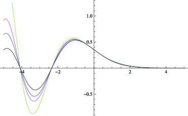
Figure 1: Product approximations of $\operatorname{Ai}(x)$.

Proposition 2.2

The functions $t\mapsto g_{c}(t)$ are in $\mathrm{PF}_{\infty}\subset\mathrm{PF}_{2}$ for every $c>0$. Thus, they are log-concave. In fact, $t\mapsto g_{c}(t)$ is strictly $\mathrm{PF}_{\infty}$ for every $c>0$.

[Proof.] By Proposition 2.1,

$$\operatorname{Ai}\bigl{(}\bigl{(}2c^{2}\bigr{)}^{-1/3}z\bigr{)} = \operatorname{Ai}(0)\mathrm{e}^{-\nu(2c^{2})^{-1/3}z}\prod_{j=1}^{\infty}\biggl{(}1+\frac{z}{(2c^{2})^{1/3}a_{j}}\biggr{)}\exp\biggl{(}-\frac{z}{(2c^{2})^{1/3}a_{j}}\biggr{)}$$

$$= \operatorname{Ai}(0)\mathrm{e}^{\delta z}\prod_{j=1}^{\infty}(1+b_{j}z)\exp(-b_{j}z),$$

which is of the form (6) required in Schoenberg’s theorem with $k=0$,

$$\delta = -\bigl{(}2c^{2}\bigr{)}^{-1/3}\nu=-\frac{(3/2)^{1/3}\Gamma(2/3)}{c^{2/3}\Gamma(1/3)},$$ (7)

$$C = \operatorname{Ai}(0)=1/\bigl{(}3^{2/3}\Gamma(2/3)\bigr{)}\quad\mbox{and}$$ (8)

$$b_{j} = \frac{1}{(2c^{2})^{1/3}a_{j}},\qquad j\geq 1,$$ (9)

where $\{-a_{j}\}$ are the zeros of the Airy function $\operatorname{Ai}$. Thus, we conclude from Schoenberg’s theorem that $g_{c}$ is $\mathrm{PF}_{\infty}$ for each $c>0$.

The strict $\mathrm{PF}_{\infty}$ property follows from Karlin [28], Theorem 6.1(a), page 357: note that in the notation of Karlin [28], $\gamma=0$ and Karlin’s $a_{i}$ is our $1/a_{k}$ with $\sum_{k}(1/a_{k})=\infty$ in view of the fact that $a_{k}\sim((3/8)\uppi(4k-1))^{2/3}$ via 9.9.6 and 9.9.18, page 18, Olver et al. [36].

Now we are in position to prove Theorem 2.1.

Proof of Theorem 2.1 This follows from Proposition 2.2: note that

$$-\log f_{Z_{c}}(x)=-\log g_{c}(x)-\log g_{c}(-x),$$

so

$$w(x)\equiv(-\log f_{Z_{c}})^{\prime\prime}(x)=(-\log g_{c})^{\prime\prime}(x)+(-\log g_{c})^{\prime\prime}(-x)\equiv v(x)+v(-x)\geq 0$$

since $g_{c}\in\mathrm{PF}_{\infty}\subset\mathrm{PF}_{2}$.

Some scaling relations: From the Fourier tranform of $g_{c}$ given above, it follows that

$$g_{c}(x) = \frac{(2/c)^{1/3}}{2\uppi}\int_{-\infty}^{\infty}\frac{\mathrm{e}^{-\mathrm{i}ux}}{\operatorname{Ai}(\mathrm{i}(2c^{2})^{-1/3}u)}\,\mathrm{d}u$$

$$= \frac{(2/c)^{1/3}(2c^{2})^{1/3}}{2\uppi}\int_{-\infty}^{\infty}\frac{\mathrm{e}^{-\mathrm{i}v(2c^{2})^{1/3}x}}{\operatorname{Ai}(\mathrm{i}v)}\,\mathrm{d}v$$

$$\equiv 2^{1/6}c^{1/3}g_{2^{-1/2}}\bigl{(}\bigl{(}2c^{2}\bigr{)}^{1/3}x\bigr{)}.$$

Thus it follows that

$$(\log g_{c})^{\prime\prime}(x)=\bigl{(}2c^{2}\bigr{)}^{2/3}\cdot(\log g_{2^{-1/2}})^{\prime\prime}\bigl{(}\bigl{(}2c^{2}\bigr{)}^{1/3}x\bigr{)},$$

and, in particular,

$$\bigl{(}\log g_{c}(x)\bigr{)}^{\prime\prime}|_{x=0}=\bigl{(}2c^{2}\bigr{)}^{2/3}\cdot(\log g_{2^{-1/2}})^{\prime\prime}(x)|_{x=0}.$$

When $c=1$, the conversion factor is $2^{2/3}$. Furthermore we compute

$$f_{Z_{c}}(t) = {\textstyle\frac{1}{2}}g_{c}(t)g_{c}(-t)={\textstyle\frac{1}{2}}2^{1/3}c^{2/3}g_{2^{-1/2}}\bigl{(}\bigl{(}2c^{2}\bigr{)}^{1/3}t\bigr{)}g_{2^{-1/2}}\bigl{(}-\bigl{(}2c^{2}\bigr{)}^{1/3}t\bigr{)}$$

$$\equiv c^{2/3}f_{1}\bigl{(}c^{2/3}t\bigr{)},$$

where

$$f_{1}(t) \equiv f_{Z_{1}}(t)={\textstyle\frac{1}{2}}g_{1}(t)g_{1}(-t)$$

$$= {\textstyle\frac{1}{2}}2^{1/3}g_{2^{-1/2}}\bigl{(}2^{1/3}t\bigr{)}g_{2^{-1/2}}\bigl{(}-2^{1/3}t\bigr{)}.$$

Thus we see that

$$Z_{c}\stackrel{{\scriptstyle d}}{{=}}c^{-2/3}Z_{1}$$

for all $c>0$.

Figure 2 gives a plot of $f_{Z}$; Figure 3 gives a plot of $-\log f_{Z}$; and Figure 4 gives a plot of $(-\log f_{Z})^{\prime\prime}$.

Figure 2: The density $f_{Z}$.

Figure 3: $-\log f_{Z}$.

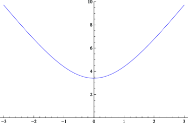
Figure 4: $(-\log f_{Z})^{\prime\prime}$.

If we use the inverse Fourier transform to represent $g$ via (4), and then calculate directly, some interesting correlation type inequalities involving the Airy kernel emerge. Here is one of them.

Let $h(u)\equiv 1/|\operatorname{Ai}(\mathrm{i}u)|\sim 2\sqrt{\uppi}u^{1/4}\exp(-(\sqrt{2}/3)u^{3/2})$ as $u\rightarrow\infty$ by Groeneboom [15], page 95. We also define $\varphi(u,x/2)=\operatorname{Re}(\mathrm{e}^{\mathrm{i}ux/2}\operatorname{Ai}(\mathrm{i}u))h(u)$ and $\psi(u,x/2)=\operatorname{Im}(\mathrm{e}^{\mathrm{i}ux/2}\times\operatorname{Ai}(\mathrm{i}u))h(u)$.

Corollary 2.1

With the above notation,

$$\int_{0}^{\infty}\sin^{2}(uy)\varphi(u,x)h(u)\,\mathrm{d}u\cdot\int_{0}^{\infty}\cos^{2}(uy)\varphi(u,x)h(u)\,\mathrm{d}u$$

$$\quad{}+\int_{0}^{\infty}\sin(uy)\cos(uy)\psi(u,x)h(u)\,\mathrm{d}u\geq 0\qquad\mbox{for all }x,y\in\mathbb{R}.$$

3 Is Chernoff’s density strongly log-concave?

From Rockafellar and Wets [40] page 565, $h\colon\ \mathbb{R}^{d}\rightarrow\overline{\mathbb{R}}$ is strongly convex if there exists a constant $c>0$ such that

$$h\bigl{(}\theta x+(1-\theta)y\bigr{)}\leq\theta h(x)+(1-\theta)h(y)-{\textstyle\frac{1}{2}}c\theta(1-\theta)\|x-y\|^{2}$$

for all $x,y\in\mathbb{R}^{d}$, $\theta\in(0,1)$. It is not hard to show that this is equivalent to convexity of

$$h(x)-{\textstyle\frac{1}{2}}c\|x\|^{2}$$

for some $c>0$. This leads (by replacing $h$ by $-\log f$) to the following definition of strong log-concavity of a (density) function: $f\mathchoice{\nobreak\,\colon}{\nobreak\,\colon}{\nobreak\,\colon\;}{\nobreak\,\colon\;}\mathbb{R}^{d}\rightarrow\overline{\mathbb{R}}$ is strongly log-concave if and only if

$$-\log f(x)-{\textstyle\frac{1}{2}}c\|x\|^{2}$$

is convex for some $c>0$. Defining $-\log g(x)\equiv-\log f(x)-(1/2)c\|x\|^{2}$, it is easily seen that $f$ is strongly log-concave if and only if

$$f(x)=g(x)\exp\bigl{(}-(1/2)c\|x\|^{2}\bigr{)}$$

for some $c>0$ and log-concave function $g$. Thus if $f\in C^{2}(\mathbb{R}^{d})$, a sufficient condition for strong log-concavity is: $\operatorname{Hess}(-\log f)(x)\geq cI_{d}$ for all $x\in\mathbb{R}^{d}$ and some $c>0$ where $I_{d}$ is the $d\times d$ identity matrix.

Figure 4 provides compelling evidence for the following conjecture concerning strong log-concavity of Chernoff’s density.

Conjecture 3.1

Let $Z_{1}$ again be a “standard” Chernoff random variable. Then for $\sigma\geq\sigma_{0}\approx 0.541912\ldots=(-(\log f_{Z_{1}}(z))^{\prime\prime}|_{z=0})^{-1/2}$ the density $f_{Z_{1}}$ can be written as

$$f_{Z_{1}}(x)=\rho(x)\frac{1}{\sigma}\varphi(x/\sigma),$$

where $\varphi(x)=(2\uppi)^{-1/2}\exp(-x^{2}/2)$ is the standard normal density and $\rho$ is log-concave. Equivalently, if $c\geq\sigma_{0}^{3/2}\approx 0.398927\ldots,$ then

$$f_{Z_{c}}(x)=\tilde{\rho}(x)\varphi(x),$$

where $\tilde{\rho}$ is log-concave.

[Proof.] (Partial) Let $w\equiv(-\log f_{Z_{c}})^{\prime\prime}$ and $v\equiv(-\log g_{c})^{\prime\prime}$. Then

$$w(t)=v(t)+v(-t)\geq 2v(0)=w(0)>0$$

is implied by convexity of $v$ and strict positivity of $w(0)$. Thus, we want to show that $v^{(2)}=(-\log g_{c})^{(4)}\geq 0$.

To prove this, we investigate the normalized version of $g_{c}$ given by $\widetilde{g}_{c}(x)=g_{c}(x)\operatorname{Ai}(0)/(2/c)^{1/3}=g_{c}(x)/\int g_{c}(y)\,\mathrm{d}y$ so that $\int\widetilde{g}_{c}(x)\,\mathrm{d}x=1$. Suppose that $b_{i}$ is given in (9), and let $X_{i}\sim\operatorname{Exp}(1/b_{i})$ be independent exponential random variables for $i=1,2,\ldots.$ Since $\sum_{i=1}^{\infty}b_{i}^{2}<\infty$, the random variable $Y_{0}=\sum_{i=1}^{\infty}(X_{i}-b_{i})$ is finite almost surely (see, e.g., Shorack [43], Theorem 9.2, page 241) and the Laplace transform of $-(\delta+Y_{0})$ is given by

$$\varphi(s) \equiv \mathrm{e}^{-\delta s}E\mathrm{e}^{-sY_{0}}=\exp(-\delta s)\cdot\frac{1}{\prod_{i=1}^{\infty}(1+b_{i}s)\mathrm{e}^{-b_{i}s}}$$

$$= \frac{1}{\mathrm{e}^{\delta s}\cdot\prod_{i=1}^{\infty}(1+b_{i}s)\mathrm{e}^{-b_{i}s}},$$

exactly the form of the Laplace transform of $g$ implicit in the proof of Proposition 2.2, but without the Gaussian term. Thus, we conclude that $\tilde{g}_{c}$ is the density of $Y\equiv-\delta-Y_{0}=-\delta-\sum_{j=1}^{\infty}(X_{j}-b_{j})$.

Now let $\lambda_{i}=1/b_{i}$ for $i\geq 1$. Thus, $X_{i}\sim\operatorname{Exp}(\lambda_{i})$. A closed form expression for the density of $Y_{m}\equiv\sum_{i=1}^{m}X_{i}$ has been given by Harrison [24]. From Harrison’s theorem 1, $Y_{m}$ has density

$$f_{m}(t)=\sum_{j=1}^{m}\lambda_{j}\exp(-\lambda_{j}t)\prod_{i\not=j}\frac{\lambda_{i}}{\lambda_{i}-\lambda_{j}}.$$ (10)

If we could show that $v_{m}(t)\equiv(-\log f_{m})^{\prime\prime}(t)$ is convex, then we would be done! Direct calculation shows that this holds for $m=2$, but our attempts at a proof for general $m$ have not (yet) been successful. On the other hand, we know that for $t\geq 0$,

$$w(t)=v(t)+v(-t)\geq v(t)\geq v(0)>0$$

if $v$ satisfies $v(t)\geq v(0)$ for all $t\geq 0$, so we would have strong log-concavity with the constant $v(0)$.

4 Discussion and open problems

Log-concavity of Chernoff’s density implies that the peakedness results of Proschan [39] and Olkin and Tong [35] apply. See also Marshall and Olkin [32], page 373, and Marshall, Olkin and Arnold [33].

Note that the conclusion of Conjecture 3.1 is exactly the form of the hypothesis of the inequality of Hargé [23] and of Theorem 11, page 559, of Caffarelli [8]; see also Barthe [4], Theorem 2.4, page 1532. Wellner [47] shows that the class of strongly log-concave densities is closed under convolution, so in particular if Conjecture 3.1 holds, then the sum of two independent Chernoff random variables is again strongly log-concave.

Another implication is that a theorem of Caffarelli [8] applies: the transportation map $T=\nabla\varphi$ is a contraction. In our particular one-dimensional special case, the transportation map $T$ satisfying $T(X)\stackrel{{\scriptstyle d}}{{=}}Z$ for $X\sim N(0,1)$ is just the solution of $\Phi(z)=F_{Z}(T(z))$, or equivalently $T(z)=F_{Z}^{-1}(\Phi(z))$. This function is apparently connected to another question concerning convex ordering of $F_{Z}$ and $\Phi(\cdot)$ in the sense of van Zwet [46]; see also van Zwet [45]: is $T^{-1}(w)=\Phi^{-1}(F_{Z}(w))$ convex for $w>0$?

As we have seen above, Chernoff’s density has the symmetric product form (2) where $g$ has Fourier transform given in (4). In this case, we know from Section 2 that $g\in\mathrm{PF}_{\infty}$.

As is shown in the longer technical report version of this paper Balabdaoui and Wellner [3], it follows from the results of Bondesson [5, 6] that the standard normal density $\phi$ can be written in the same structural form as that of Chernoff’s density (2); that is:

$$\phi(z)={\textstyle\frac{1}{2}}g(z)g(-z),$$ (11)

where now

$$g(z) \equiv (2/\uppi)^{1/4}\exp(z)\exp\biggl{(}\int_{0}^{\infty}\log\biggl{(}\frac{\mathrm{e}^{s}+1}{\mathrm{e}^{s}+\mathrm{e}^{z}}\biggr{)}\,\mathrm{d}s\biggr{)}$$

$$= (2/\uppi)^{1/4}\exp\biggl{(}\frac{\uppi^{2}}{12}+z-\int_{0}^{\mathrm{e}^{z}}\frac{\log(1+t)}{t}\,\mathrm{d}t\biggr{)}$$

is log-concave, integrable, and $g\in\log(\mathrm{HM}_{\infty})$, the log-transform (in terms of random variables) of the Hyperbolically Completely Monotone class of Bondesson [5, 6]. Two natural questions are: (a) Does the function $g$ in (2) satisfy $g\in\log(\mathrm{HM}_{\infty})$? (b) Does the function $g$ in (4) satisfy $g\in\mathrm{PF}_{\infty}$?

A further question remaining from Section 3: Is Chernoff’s density strongly log-concave?

A whole class of further problems involves replacing the (ordered) convex cone $K_{n}$ in Section 1 by the convex cone $\widetilde{\mathcal{K}}_{n}$ corresponding to a convexity restriction as in Section 2 of Groeneboom, Jongbloed and Wellner [20]. In this latter case, the limiting distribution depends on an “invelope” of the integral of a two-sided Brownian motion plus a polynomial drift as follows: it is the density of the second derivative at zero of the “invelope”. See Groeneboom, Jongbloed and Wellner [20, 19] for further details and Balabdaoui, Rufibach and Wellner [2] for another convexity related shape constraint where this limiting distribution occurs. However, virtually nothing is known concerning the analytical properties of this distribution.

References

- [1] {barticle}[mr] \bauthor\bsnmAyer, \bfnmMiriam\binitsM., \bauthor\bsnmBrunk, \bfnmH. D.\binitsH.D., \bauthor\bsnmEwing, \bfnmG. M.\binitsG.M., \bauthor\bsnmReid, \bfnmW. T.\binitsW.T. &\bauthor\bsnmSilverman, \bfnmEdward\binitsE. (\byear1955). \btitleAn empirical distribution function for sampling with incomplete information. \bjournalAnn. Math. Statist. \bvolume26 \bpages641–647. \bidissn=0003-4851, mr=0073895 \bptokimsref \endbibitem
- [2] {barticle}[mr] \bauthor\bsnmBalabdaoui, \bfnmFadoua\binitsF., \bauthor\bsnmRufibach, \bfnmKaspar\binitsK. &\bauthor\bsnmWellner, \bfnmJon A.\binitsJ.A. (\byear2009). \btitleLimit distribution theory for maximum likelihood estimation of a log-concave density. \bjournalAnn. Statist. \bvolume37 \bpages1299–1331. \biddoi=10.1214/08-AOS609, issn=0090-5364, mr=2509075 \bptokimsref \endbibitem
- [3] {bmisc}[author] \bauthor\bsnmBalabdaoui, \bfnmFadoua\binitsF. &\bauthor\bsnmWellner, \bfnmJon A.\binitsJ.A. (\byear2012). \bhowpublishedChernoff’s distribution is log-concave. Technical Report No. tr595.pdf. Dept. Statistics, Univ. Washington. Available at arXiv:\arxivurl1203.0828v1. \bptokimsref \endbibitem
- [4] {bincollection}[mr] \bauthor\bsnmBarthe, \bfnmFranck\binitsF. (\byear2006). \btitleThe Brunn–Minkowski theorem and related geometric and functional inequalities. In \bbooktitleInternational Congress of Mathematicians. Vol. II \bpages1529–1546. \blocationZürich: \bpublisherEur. Math. Soc. \bidmr=2275657 \bptokimsref \endbibitem
- [5] {bbook}[mr] \bauthor\bsnmBondesson, \bfnmLennart\binitsL. (\byear1992). \btitleGeneralized Gamma Convolutions and Related Classes of Distributions and Densities. \bseriesLecture Notes in Statistics \bvolume76. \blocationNew York: \bpublisherSpringer. \biddoi=10.1007/978-1-4612-2948-3, mr=1224674 \bptokimsref \endbibitem
- [6] {bincollection}[mr] \bauthor\bsnmBondesson, \bfnmLennart\binitsL. (\byear1997). \btitleOn hyperbolically monotone densities. In \bbooktitleAdvances in the Theory and Practice of Statistics. \bseriesWiley Ser. Probab. Statist. Appl. Probab. Statist. \bpages299–313. \blocationNew York: \bpublisherWiley. \bidmr=1481175 \bptokimsref \endbibitem
- [7] {bincollection}[mr] \bauthor\bsnmBrunk, \bfnmH. D.\binitsH.D. (\byear1970). \btitleEstimation of isotonic regression. In \bbooktitleNonparametric Techniques in Statistical Inference (Proc. Sympos., Indiana Univ., Bloomington, Ind., 1969) \bpages177–197. \blocationLondon: \bpublisherCambridge Univ. Press. \bidmr=0277070 \bptokimsref \endbibitem
- [8] {barticle}[mr] \bauthor\bsnmCaffarelli, \bfnmLuis A.\binitsL.A. (\byear2000). \btitleMonotonicity properties of optimal transportation and the FKG and related inequalities. \bjournalComm. Math. Phys. \bvolume214 \bpages547–563. \biddoi=10.1007/s002200000257, issn=0010-3616, mr=1800860 \bptokimsref \endbibitem
- [9] {barticle}[mr] \bauthor\bsnmChernoff, \bfnmHerman\binitsH. (\byear1964). \btitleEstimation of the mode. \bjournalAnn. Inst. Statist. Math. \bvolume16 \bpages31–41. \bidissn=0020-3157, mr=0172382 \bptokimsref \endbibitem
- [10] {barticle}[mr] \bauthor\bsnmDaniels, \bfnmH. E.\binitsH.E. &\bauthor\bsnmSkyrme, \bfnmT. H. R.\binitsT.H.R. (\byear1985). \btitleThe maximum of a random walk whose mean path has a maximum. \bjournalAdv. in Appl. Probab. \bvolume17 \bpages85–99. \biddoi=10.2307/1427054, issn=0001-8678, mr=0778595 \bptokimsref \endbibitem
- [11] {bbook}[mr] \bauthor\bsnmDehling, \bfnmHerold\binitsH. &\bauthor\bsnmPhilipp, \bfnmWalter\binitsW. (\byear2002). \btitleEmpirical Process Techniques for Dependent Data. \blocationBoston, MA: \bpublisherBirkhäuser. \biddoi=10.1007/978-1-4612-0099-4, mr=1958776 \bptokimsref \endbibitem
- [12] {barticle}[mr] \bauthor\bsnmGrenander, \bfnmUlf\binitsU. (\byear1956). \btitleOn the theory of mortality measurement. I. \bjournalSkand. Aktuarietidskr. \bvolume39 \bpages70–96. \bidmr=0086459 \bptokimsref \endbibitem
- [13] {barticle}[mr] \bauthor\bsnmGrenander, \bfnmUlf\binitsU. (\byear1956). \btitleOn the theory of mortality measurement. II. \bjournalSkand. Aktuarietidskr. \bvolume39 \bpages125–153. \bidmr=0093415 \bptokimsref \endbibitem
- [14] {binproceedings}[mr] \bauthor\bsnmGroeneboom, \bfnmP.\binitsP. (\byear1985). \btitleEstimating a monotone density. In \bbooktitleProceedings of the Berkeley Conference in Honor of Jerzy Neyman and Jack Kiefer, Vol. II (Berkeley, CA, 1983). \bseriesWadsworth Statist./Probab. Ser. \bpages539–555. \blocationBelmont, CA: \bpublisherWadsworth. \bidmr=0822052 \bptokimsref \endbibitem
- [15] {barticle}[mr] \bauthor\bsnmGroeneboom, \bfnmPiet\binitsP. (\byear1989). \btitleBrownian motion with a parabolic drift and Airy functions. \bjournalProbab. Theory Related Fields \bvolume81 \bpages79–109. \biddoi=10.1007/BF00343738, issn=0178-8051, mr=0981568 \bptokimsref \endbibitem
- [16] {bincollection}[mr] \bauthor\bsnmGroeneboom, \bfnmPiet\binitsP. (\byear1996). \btitleLectures on inverse problems. In \bbooktitleLectures on Probability Theory and Statistics (Saint-Flour, 1994). \bseriesLecture Notes in Math. \bvolume1648 \bpages67–164. \blocationBerlin: \bpublisherSpringer. \biddoi=10.1007/BFb0095675, mr=1600884 \bptokimsref \endbibitem
- [17] {barticle}[mr] \bauthor\bsnmGroeneboom, \bfnmPiet\binitsP. (\byear2010). \btitleThe maximum of Brownian motion minus a parabola. \bjournalElectron. J. Probab. \bvolume15 \bpages1930–1937. \biddoi=10.1214/EJP.v15-826, issn=1083-6489, mr=2738343 \bptokimsref \endbibitem
- [18] {barticle}[mr] \bauthor\bsnmGroeneboom, \bfnmPiet\binitsP. (\byear2011). \btitleVertices of the least concave majorant of Brownian motion with parabolic drift. \bjournalElectron. J. Probab. \bvolume16 \bpages2234–2258. \biddoi=10.1214/EJP.v16-959, issn=1083-6489, mr=2861676 \bptokimsref \endbibitem
- [19] {barticle}[mr] \bauthor\bsnmGroeneboom, \bfnmPiet\binitsP., \bauthor\bsnmJongbloed, \bfnmGeurt\binitsG. &\bauthor\bsnmWellner, \bfnmJon A.\binitsJ.A. (\byear2001). \btitleA canonical process for estimation of convex functions: The “invelope” of integrated Brownian motion . \bjournalAnn. Statist. \bvolume29 \bpages1620–1652. \biddoi=10.1214/aos/1015345957, issn=0090-5364, mr=1891741 \bptokimsref \endbibitem
- [20] {barticle}[mr] \bauthor\bsnmGroeneboom, \bfnmPiet\binitsP., \bauthor\bsnmJongbloed, \bfnmGeurt\binitsG. &\bauthor\bsnmWellner, \bfnmJon A.\binitsJ.A. (\byear2001). \btitleEstimation of a convex function: Characterizations and asymptotic theory. \bjournalAnn. Statist. \bvolume29 \bpages1653–1698. \biddoi=10.1214/aos/1015345958, issn=0090-5364, mr=1891742 \bptokimsref \endbibitem
- [21] {bbook}[mr] \bauthor\bsnmGroeneboom, \bfnmPiet\binitsP. &\bauthor\bsnmWellner, \bfnmJon A.\binitsJ.A. (\byear1992). \btitleInformation Bounds and Nonparametric Maximum Likelihood Estimation. \bseriesDMV Seminar \bvolume19. \blocationBasel: \bpublisherBirkhäuser. \biddoi=10.1007/978-3-0348-8621-5, mr=1180321 \bptokimsref \endbibitem
- [22] {barticle}[mr] \bauthor\bsnmGroeneboom, \bfnmPiet\binitsP. &\bauthor\bsnmWellner, \bfnmJon A.\binitsJ.A. (\byear2001). \btitleComputing Chernoff’s distribution. \bjournalJ. Comput. Graph. Statist. \bvolume10 \bpages388–400. \biddoi=10.1198/10618600152627997, issn=1061-8600, mr=1939706 \bptokimsref \endbibitem
- [23] {barticle}[mr] \bauthor\bsnmHargé, \bfnmGilles\binitsG. (\byear2004). \btitleA convex/log-concave correlation inequality for Gaussian measure and an application to abstract Wiener spaces. \bjournalProbab. Theory Related Fields \bvolume130 \bpages415–440. \biddoi=10.1007/s00440-004-0365-8, issn=0178-8051, mr=2095937 \bptokimsref \endbibitem
- [24] {barticle}[mr] \bauthor\bsnmHarrison, \bfnmPeter G.\binitsP.G. (\byear1990). \btitleLaplace transform inversion and passage-time distributions in Markov processes. \bjournalJ. Appl. Probab. \bvolume27 \bpages74–87. \bidissn=0021-9002, mr=1039185 \bptokimsref \endbibitem
- [25] {barticle}[mr] \bauthor\bsnmHuang, \bfnmJian\binitsJ. &\bauthor\bsnmWellner, \bfnmJon A.\binitsJ.A. (\byear1995). \btitleEstimation of a monotone density or monotone hazard under random censoring. \bjournalScand. J. Stat. \bvolume22 \bpages3–33. \bidissn=0303-6898, mr=1334065 \bptokimsref \endbibitem
- [26] {barticle}[mr] \bauthor\bsnmHuang, \bfnmYouping\binitsY. &\bauthor\bsnmZhang, \bfnmCun-Hui\binitsC.H. (\byear1994). \btitleEstimating a monotone density from censored observations. \bjournalAnn. Statist. \bvolume22 \bpages1256–1274. \biddoi=10.1214/aos/1176325628, issn=0090-5364, mr=1311975 \bptokimsref \endbibitem
- [27] {barticle}[mr] \bauthor\bsnmJanson, \bfnmSvante\binitsS., \bauthor\bsnmLouchard, \bfnmGuy\binitsG. &\bauthor\bsnmMartin-Löf, \bfnmAnders\binitsA. (\byear2010). \btitleThe maximum of Brownian motion with parabolic drift. \bjournalElectron. J. Probab. \bvolume15 \bpages1893–1929. \biddoi=10.1214/EJP.v15-830, issn=1083-6489, mr=2738342 \bptokimsref \endbibitem
- [28] {bbook}[mr] \bauthor\bsnmKarlin, \bfnmSamuel\binitsS. (\byear1968). \btitleTotal Positivity. Vol. I. \blocationStanford, CA: \bpublisherStanford Univ. Press. \bidmr=0230102 \bptokimsref \endbibitem
- [29] {barticle}[mr] \bauthor\bsnmKim, \bfnmJeanKyung\binitsJ. &\bauthor\bsnmPollard, \bfnmDavid\binitsD. (\byear1990). \btitleCube root asymptotics. \bjournalAnn. Statist. \bvolume18 \bpages191–219. \biddoi=10.1214/aos/1176347498, issn=0090-5364, mr=1041391 \bptokimsref \endbibitem
- [30] {barticle}[mr] \bauthor\bsnmLe Cam, \bfnmL.\binitsL. (\byear1986). \btitleThe central limit theorem around 1935. \bjournalStatist. Sci. \bvolume1 \bpages78–96. \bidissn=0883-4237, mr=0833276 \bptokimsref \endbibitem
- [31] {barticle}[mr] \bauthor\bsnmLeurgans, \bfnmSue\binitsS. (\byear1982). \btitleAsymptotic distributions of slope-of-greatest-convex-minorant estimators. \bjournalAnn. Statist. \bvolume10 \bpages287–296. \bidissn=0090-5364, mr=0642740 \bptokimsref \endbibitem
- [32] {bbook}[mr] \bauthor\bsnmMarshall, \bfnmAlbert W.\binitsA.W. &\bauthor\bsnmOlkin, \bfnmIngram\binitsI. (\byear1979). \btitleInequalities: Theory of Majorization and Its Applications. \bseriesMathematics in Science and Engineering \bvolume143. \blocationNew York: \bpublisherAcademic Press [Harcourt Brace Jovanovich Publishers]. \bidmr=0552278 \bptokimsref \endbibitem
- [33] {bbook}[mr] \bauthor\bsnmMarshall, \bfnmAlbert W.\binitsA.W., \bauthor\bsnmOlkin, \bfnmIngram\binitsI. &\bauthor\bsnmArnold, \bfnmBarry C.\binitsB.C. (\byear2011). \btitleInequalities: Theory of Majorization and Its Applications, \bedition2nd ed. \bseriesSpringer Series in Statistics. \blocationNew York: \bpublisherSpringer. \biddoi=10.1007/978-0-387-68276-1, mr=2759813 \bptokimsref \endbibitem
- [34] {barticle}[mr] \bauthor\bsnmMerkes, \bfnmE. P.\binitsE.P. &\bauthor\bsnmSalmassi, \bfnmMohammad\binitsM. (\byear1997). \btitleOn univalence of certain infinite products. \bjournalComplex Variables Theory Appl. \bvolume33 \bpages207–215. \bidissn=0278-1077, mr=1624939 \bptokimsref \endbibitem
- [35] {bincollection}[mr] \bauthor\bsnmOlkin, \bfnmI.\binitsI. &\bauthor\bsnmTong, \bfnmY. L.\binitsY.L. (\byear1988). \btitlePeakedness in multivariate distributions. In \bbooktitleStatistical Decision Theory and Related Topics, IV, Vol. 2 (West Lafayette, IN, 1986) \bpages373–383. \blocationNew York: \bpublisherSpringer. \bidmr=0927147 \bptokimsref \endbibitem
- [36] {bbook}[mr] \bauthor\bsnmOlver, \bfnmF. W. J.\binitsF.W.J., \bauthor\bsnmLozier, \bfnmD. W.\binitsD.W., \bauthor\bsnmBoisvert, \bfnmR. F.\binitsR.F. &\bauthor\bsnmClark, \bfnmCh. W.\binitsC.W. (\byear2010). \btitleNIST Handbook of Mathematical Functions. \blocationWashington, DC: \bpublisherU.S. Department of Commerce National Institute of Standards and Technology. \bidmr=2723248 \bptokimsref \endbibitem
- [37] {barticle}[mr] \bauthor\bsnmPrakasa Rao, \bfnmB. L. S.\binitsB.L.S. (\byear1969). \btitleEstkmation of a unimodal density. \bjournalSankhyā Ser. A \bvolume31 \bpages23–36. \bidissn=0581-572X, mr=0267677 \bptokimsref \endbibitem
- [38] {barticle}[mr] \bauthor\bsnmPrakasa Rao, \bfnmB. L. S.\binitsB.L.S. (\byear1970). \btitleEstimation for distributions with monotone failure rate. \bjournalAnn. Math. Statist. \bvolume41 \bpages507–519. \bidissn=0003-4851, mr=0260133 \bptokimsref \endbibitem
- [39] {barticle}[mr] \bauthor\bsnmProschan, \bfnmFrank\binitsF. (\byear1965). \btitlePeakedness of distributions of convex combinations. \bjournalAnn. Math. Statist. \bvolume36 \bpages1703–1706. \bidissn=0003-4851, mr=0187269 \bptokimsref \endbibitem
- [40] {bbook}[mr] \bauthor\bsnmRockafellar, \bfnmR. Tyrrell\binitsR.T. &\bauthor\bsnmWets, \bfnmRoger J. B.\binitsR.J.B. (\byear1998). \btitleVariational Analysis. \bseriesGrundlehren der Mathematischen Wissenschaften [Fundamental Principles of Mathematical Sciences] \bvolume317. \blocationBerlin: \bpublisherSpringer. \biddoi=10.1007/978-3-642-02431-3, mr=1491362 \bptokimsref \endbibitem
- [41] {barticle}[mr] \bauthor\bsnmSalmassi, \bfnmMohammad\binitsM. (\byear1999). \btitleInequalities satisfied by the Airy functions. \bjournalJ. Math. Anal. Appl. \bvolume240 \bpages574–582. \biddoi=10.1006/jmaa.1999.6620, issn=0022-247X, mr=1731663 \bptokimsref \endbibitem
- [42] {barticle}[mr] \bauthor\bsnmSchoenberg, \bfnmI. J.\binitsI.J. (\byear1951). \btitleOn Pólya frequency functions. I. The totally positive functions and their Laplace transforms. \bjournalJ. Anal. Math. \bvolume1 \bpages331–374. \bidissn=0021-7670, mr=0047732 \bptokimsref \endbibitem
- [43] {bbook}[mr] \bauthor\bsnmShorack, \bfnmGalen R.\binitsG.R. (\byear2000). \btitleProbability for Statisticians. \bseriesSpringer Texts in Statistics. \blocationNew York: \bpublisherSpringer. \bidmr=1762415 \bptokimsref \endbibitem
- [44] {barticle}[mr] \bauthor\bparticlevan \bsnmEeden, \bfnmConstance\binitsC. (\byear1957). \btitleMaximum likelihood estimation of partially or completely ordered parameters. I. \bjournalNederl. Akad. Wetensch. Proc. Ser. A. 60 = Indag. Math. \bvolume19 \bpages128–136. \bidmr=0083869 \bptokimsref \endbibitem
- [45] {barticle}[mr] \bauthor\bparticlevan \bsnmZwet, \bfnmW. R.\binitsW.R. (\byear1964). \btitleConvex transformations: A new approach to skewness and kurtosis. \bjournalStat. Neerl. \bvolume18 \bpages433–441. \bidissn=0039-0402, mr=0175217 \bptokimsref \endbibitem
- [46] {bbook}[mr] \bauthor\bparticlevan \bsnmZwet, \bfnmW. R.\binitsW.R. (\byear1964). \btitleConvex Transformations of Random Variables. \bseriesMathematical Centre Tracts \bvolume7. \blocationAmsterdam: \bpublisherMathematisch Centrum. \bidmr=0176511 \bptokimsref \endbibitem
- [47] {bmisc}[author] \bauthor\bsnmWellner, \bfnmJon A.\binitsJ.A. (\byear2013). \bhowpublishedStrong log-concavity is preserved by convolution. In High Dimensional Probability VI: The Banff Volume (Progress in Probability) (C. Houdré, D. M. Mason, J. Rosiński and J. A. Wellner, eds.) 95–103. Basel: Birkhauser. \bptokimsref \endbibitem