Vacuum Pressure Measurements using a Magneto-Optical Trap

Abstract

The loading dynamics of an alkali-atom magneto-optical trap can be used as a reliable measure of vacuum pressure, with loading time $\tau$ indicating a pressure less than or equal to ($2\times 10^{-8}$ Torr s)/$\tau$. This relation is accurate to approximately a factor of two over wide variations in trap parameters, background gas composition, or trapped alkali species. The low-pressure limit of the method does depend on the trap parameters, but typically extends to the $10^{-10}$ Torr range.

I Introduction

The use of ultra-high vacuum (UHV) systems is ubiquitous in modern atomic physics. Vacuum practices and technologies sufficient to attain pressures on the order of $10^{-9}$ Torr or lower are well known Lafferty (1998), but nonetheless often comprise a significant experimental complexity. In addition, the space and power requirements of UHV systems can be considered a barrier to the development of commercial applications based on atomic physics techniques. While the primary concern in such systems is the generation and maintenance of UHV pressures, an important secondary issue is the measurement of pressure.

The standard instrument for UHV pressure measurement is the ionization gauge Lafferty (1998), which takes various forms and can measure pressures to $10^{-11}$ Torr or lower Watanabe (1999). However, ionization gauges require typically 100 W of electrical power, and take up volumes of 100 cm³ or more. These requirements may be negligible in large laboratory-based vacuum systems, but as systems are miniaturized and streamlined to improve simplicity and efficiency, ionization gauges are likely to become unacceptable. Another measurement instrument, the residual gas analyzer, suffers from similar constraints.

An alternative technique is to measure vacuum pressure using an ion pump Lafferty (1998); Welch (2001). Ion pumps are primarily used to maintain vacuum pressure, but measurement of the pump current provides a pressure indicator as well. Ion pumps do not generally perform as well as ionization gauges, since leakage currents limit the minimum pressure reading, typically in the $10^{-9}$ Torr range. The relation between current and pressure is also complicated and varies with pump design. Finally, ion pumps are themselves typically large and power intensive, and they require a significant magnetic field near the pump, all of which can be drawbacks in some applications DAR . Pumping methods such as evaporable and non-evaporable getters, turbopumps, and cryopumps could avoid such problems or be preferred for other reasons. None of these techniques provides a pressure measurement facility.

It is the purpose of this paper to explore the extent to which the experiment itself can provide a pressure measurement. In particular, we consider the magneto-optical trap (MOT), which is the starting point for many atomic physics experiments and applications. We find that measurement of the MOT loading time can serve as a useful and reasonably accurate pressure gauge, but that lifetime limits imposed by collisions between the trapped atoms give a low pressure floor in the $10^{-10}$ Torr range. The technique has resolution comparable to an ion pump measurement, but avoids the drawbacks mentioned above. The method can be used for both beam-loaded and vapor-cell loaded traps.

We note at the outset that we do not strive here for a high-accuracy pressure measurement. In some cases high accuracy is important, but a significant calibration uncertainty is usually acceptable for vacuum diagnostic purposes. For instance, the sensitivity of an ionization gauge varies by a factor of two between H₂ and N₂ gases, and by a factor of eight between He and Ar Lafferty (1998). Ion pump sensitivities show similar or greater variation Welch (2001). These effects lead to significant uncertainty if the residual gas composition is not known. Nonetheless, both ionization gauges and ion pumps have proven satisfactory for many applications. We show here that MOT loading measurements can provide an accuracy of about a factor of two, comparable to that typically obtained with conventional techniques.

The basic connection between MOT dynamics and background gas pressure has been understood since MOTs were developed Raab et al. (1987); Prentiss et al. (1988); Bjorkholm (1988), but to our knowledge MOTs have not previously been proposed for providing quantitative pressure measurements. This can likely be explained by the common availability of standard measurement gauges. In addition, it is evident that the relationship between background pressure and MOT dynamics will depend on the trap depth of the MOT. The trap depth varies considerably with the laser parameters used and can be challenging to quantify. This would weigh against using the MOT as a measurement tool, since calibration would be difficult and uncertain.

As noted by Bjorkholm Bjorkholm (1988), however, the dependence of loading time on trap depth is in fact quite weak under most conditions. Furthermore, the loading time depends only weakly on the type of atom being trapped and the composition of the background gas. In light of this, a “universal” pressure calibration is in fact possible so long as high accuracy is not required. Thus MOT measurements can serve as a convenient general-purpose measurement tool.

A similar technique was previously used by Willems and Libbrecht Willems and Libbrecht (1995) to relate the loss rate from a magnetic trap to the pressure in a cryogenic vacuum system. Also, collisional loss rates at a known background gas density and MOT trap depth have been used to characterize collision cross sections Cable et al. (1990); Matherson et al. (2008); Fagnan et al. (2009), or alternatively collision rates at a known cross section and gas density can be used to characterize the MOT trap depth Van Dongen et al. (2011).

II Theory

The dynamics of MOT loading and loss are governed, to a good approximation, by the rate equation

$$\frac{dN}{dt}=R-\gamma N(t)-\beta\bar{n}N(t).$$ (1)

Here $N$ is the number of atoms in the trap and $R$ is the rate at which atoms are loaded via laser cooling. Normally, $R$ will be proportional to the background gas pressure of the species being trapped. The trap losses are described by $\gamma$, the rate constant for loss due to collisions with all background gases, and $\beta$, the rate constant for loss due to inelastic two-body collisions within the trap. The two-body rate also depends on the mean density of the trapped atoms, $\bar{n}=(1/N)\int n({\bf r})^{2}d^{3}r$.

In order to solve (1), the variation of $\bar{n}$ with $N$ must be known, which can be complicated in general. Typically two regimes are identified, depending on the significance of multiple-scattering forces within the MOT Sesko et al. (1991); Townsend et al. (1995); Overstreet et al. (2005). For small $N$, less than of order $10^{5}$ atoms, the scattering forces are weak and $\bar{n}\approx N(t)/V$ with fixed trap volume $V$. For larger $N$, light scattering enforces a constant $\bar{n}$ with $V\propto N$. In the constant density limit, (1) results in an exponential loading curve

$$N=\frac{R}{\Gamma}(1-e^{-\Gamma t})$$ (2)

with

$$\Gamma=\gamma+\beta\bar{n}.$$ (3)

An exponential curve is also observed in the constant volume regime if $\gamma\gg\beta\bar{n}$, which is often the case since $N$ is small. For nearly all the parameters we investigated, the observed loading curves were exponential to a good approximation. Figure 1 shows an example.

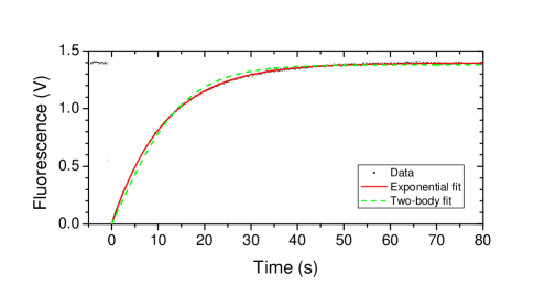
Figure 1: (color online) MOT loading dynamics. The vertical axis shows the atomic fluorescence as measured by a photodiode, after the cooling beams are briefly blocked at time $t=0$. Data points are the experimentally measured values for a ⁸⁷Rb trap holding a maximum of $3\times 10^{8}$ atoms. The solid (red) curve that lies on top of the data is a fit to the exponential form of (2). For comparison, the dashed (green) curve is a fit to $N(t)=\sqrt{RV/\beta}\tanh(t\sqrt{R\beta/V})$, the solution to (1) in the limit of constant volume $V$ and $\gamma\rightarrow 0$.

By measuring a curve such as Fig. 1, $R$ and $\Gamma$ can readily be determined. To the extent that $\beta\bar{n}$ can be controlled or neglected, this provides knowledge of $\gamma$, which is directly related to the background gas density and thus the pressure. The practical impact of the $\beta\bar{n}$ term on the pressure measurement will be discussed in Section IV below.

The loss coefficient $\gamma$ can generally be expressed as

$$\gamma=\sum_{i}n_{i}\langle\sigma_{i}v_{i}\rangle$$ (4)

where the sum is over gas species $i$, with density $n_{i}$, speed $v_{i}$, and loss cross section $\sigma_{i}$. The angle brackets represent an average over the thermal distribution, and we assume that the velocity of the trapped atoms is negligible compared to $v_{i}$. The loss cross section $\sigma_{i}$ is given by

$$\sigma_{i}=\int_{\theta>\theta_{L}}\frac{d\sigma}{d\Omega}d\Omega$$ (5)

where $d\sigma/d\Omega$ is the differential scattering cross section and $\theta_{L}$ is the minimum scattering angle required in order to give the target cold atom sufficient energy to escape the trap.

The long-range interaction potential between ground state trapped atoms and background species $i$ can typically be approximated with the van der Waals form $-C_{i}/r^{6}$ Margenau and Kestner (1969). The trapped atoms do have some amplitude to be in an excited state, which typically modifies the $C_{i}$ coefficient. For interactions between excited atoms and background atoms of the same species the interaction can be significantly enhanced to an $r^{-3}$ form. We will neglect this effect for now, since our main interest will be losses due to vacuum contamination by non-trapped species.

Typical MOT trap depths $D$ are on the order of 1 K, which is large enough that the cross section can be estimated classically but small enough that the small angle and impulse approximations can be used Bjorkholm (1988); Bali et al. (1999). For a van der Waals potential this leads to

$$\frac{d\sigma}{d\Omega}=\frac{1}{6}\left(\frac{15\pi}{8}\frac{C_{i}}{m_{i}v_{i}^{2}}\right)^{1/3}\theta^{-7/3}$$ (6)

where $m_{i}$ is the mass of the incident species. The critical angle $\theta_{L}$ is $\sqrt{2m_{0}D}/(m_{i}v_{i})$ for trapped atom mass $m_{0}$. Evaluating (5) then gives

$$\sigma_{i}=\left(\frac{15\pi^{4}}{16}\right)^{1/3}\left(\frac{m_{i}C_{i}^{2}}{m_{0}E_{i}D}\right)^{1/6}$$ (7)

for incident energy $E_{i}=m_{i}v_{i}^{2}/2$. Finally, $\sigma_{i}v_{i}$ can be averaged over a Maxwell-Boltzmann distribution at temperature $T$, and the density $n_{i}$ can be expressed in terms of the partial pressure $P_{i}=n_{i}k_{B}T$. This yields the loss rate Bjorkholm (1988)

$$\gamma_{i}\approx 6.8\frac{P_{i}}{(k_{B}T)^{2/3}}\left(\frac{C_{i}}{m_{i}}\right)^{1/3}(Dm_{0})^{-1/6}.$$ (8)

Thus, as claimed in Section I, $\gamma_{i}$ depends only weakly on the trap depth $D$. Gensemer et al. and Van Dongen et al. measured loss rate variations consistent with this dependence for trap depths between 0.5 and 2 K Gensemer et al. (1997); Van Dongen et al. (2011), a range consistent with other reported trap depth measurements for alkali atoms Raab et al. (1987); Kawanaka et al. (1993); Hoffmann et al. (1996); Bagnato et al. (2000). For the purpose of pressure measurement, we see that the loss calibration does not vary significantly with trap parameters such as laser intensity and detuning. Note, however, that for smaller trap depths the loss rate can vary more significantly as the validity of the classical approximation starts to fail Gensemer et al. (1997); Bali et al. (1999); Van Dongen et al. (2011).

The loss coefficient depends on the background gas species through $C_{i}$ and $m_{i}$. The van der Walls coefficients $C_{i}$ can be estimated using the Slater-Kirkwood formula Margenau and Kestner (1969); Miller and Bederson (1977),

$$C_{i}=\frac{3}{2}\frac{\hbar e}{(4\pi\epsilon_{0})^{2}m_{e}^{1/2}}\frac{\alpha_{0}\alpha_{i}}{(\alpha_{0}/\rho_{0})^{1/2}+(\alpha_{i}/\rho_{i})^{1/2}}$$ (9)

where $m_{e}$ is the electron mass and species $i$ has static electric polarizability $\alpha_{i}$ and number of valence electrons $\rho_{i}$. As above, $i=0$ refers to the trapped species. Typically, the polarizability of a particle increases with its mass, so the variation in $C_{i}/m_{i}$ is reduced compared to that of $C_{i}$ or $m_{i}$ alone. Table 1 shows the calculated loss coefficents for trapped Rb atoms caused by various background gas species.

We noted previously that excited atoms generally have a different $C_{i}$ coefficient. In reference to (9), the dc polarizability of alkali atoms in their first excited states is typically 2–4 times larger than that for the ground state Miller and Bederson (1977). However, the ground-state polarizability of the alkalis is already very large, so for interactions with non-alkali species, the $\alpha_{0}/\rho_{0}$ term in the denominator typically dominates $\alpha_{i}/\rho_{i}$. The $C_{i}$ coefficient therefore scales approximately as $\alpha_{0}^{1/2}$ and the loss rate as $\alpha_{0}^{1/6}$. The loss rate coefficients can therefore be expected to differ by not more than 30% from the ground estimates, with the caveat that resonant interactions can be expected to give larger deviations for collisions with hot atoms of the same species as those trapped.

Finally, the loss coefficients depends only weakly on the trapped atom species itself, as seen in Table 2. Note, however, that the classical scattering approximation may be inadequate for lithium atoms in a shallow MOT Bali et al. (1999), leading to a stronger dependence on the trap depth.

Species		$C_{i}$	$\gamma_{i}/P$
H2		137 a.u.	$4.9\times 10^{7}$ Torr-1 s-1
He		35	2.5$\times 10^{7}$
H2O		241	2.8$\times 10^{7}$
N2		302	2.6$\times 10^{7}$
Ar		278	2.3$\times 10^{7}$
CO2		482	2.6$\times 10^{7}$
Rb		4400	4.4$\times 10^{7}$

Table 1: Estimated loss coefficients for collisions between ground-state Rb atoms and the indicated background gas, for a 1 K trap depth and 300 K background gas temperature. The $C_{i}$ coefficients are in atomic units, calculated using (9). The loss coefficients $\gamma_{i}/P$ are calculated from Eq. (8).

Species		$C_{\mbox{\scriptsize H${}_{2}$}}$	$\gamma_{\mbox{\scriptsize H${}_{2}$}}/P$
Li		82.5 a.u.	$6.4\times 10^{7}$ Torr-1 s-1
Na		91	5.3$\times 10^{7}$
K		130	5.4$\times 10^{7}$
Rb		140	4.9$\times 10^{7}$
Cs		170	4.9$\times 10^{7}$

Table 2: Estimated loss rate coefficients for collisions between ground-state alkali atoms and hydrogen molecules, for a 1 K trap depth and 300 K background gas temperature. The $C_{\mbox{\scriptsize H${}_{2}$}}$ coefficients are in atomic units, taken from Bali et al. (1999). The loss coefficients are calculated from Eq. (8).

We conclude that in most cases, the relation between loss rate and background pressure is expected to vary by only a factor of about two. For pressure measurement, this level of variation is generally acceptable and in fact rather better than that of conventional pressure gauges.

III Measurements

Clear experimental measurements of $\partial\gamma/\partial P$ are not common in the literature. Prentiss et al. made an early measurement $\gamma/P=5\times 10^{7}$ Torr^-1 s^-1 in a sodium MOT likely dominated by H₂ background gas Prentiss et al. (1988). More recently, Fagnan et al. Fagnan et al. (2009) and Van Dongen et al. Van Dongen et al. (2011) measured the dependence of the collisional loss in a Rb MOT on the partial pressure of Ar gas. For a trap depth of 1 K, Fagnan obtained $\gamma_{\mbox{\scriptsize Ar}}/P=1.6\times 10^{7}$ Torr^-1 s^-1 while Van Dongen obtained $2.2\times 10^{7}$ Torr^-1 s^-1. Both Ar measurements were in good agreement with a fully quantum calculation of the loss rate. As seen in Tables 1 and 2, our classical calculation also agrees with all of these results.

To test the relationship between vacuum pressure and loss rate ourselves, we experimentally investigated the loading dynamics in a rubidium MOT. The majority of the experiments were performed in a vacuum chamber consisting of a 30-cm long, 6-cm diameter cylindrical glass cell that is connected to a second cell by a 20-cm long, 1-cm diameter tube. The MOT was produced and studied in the cylindrical cell; the second cell is designed for the production of Bose-Einstein condensates. The MOT cell is mounted on a stainless steel cross, to which is also attached a 20 L/s ion pump from Duniway Stockroom and a tubulated Bayard-Alpert ionization gauge. The unused cell is pumped by a 20 L/s Varian ion pump. The vacuum conduction between the two cells is estimated as 0.5 L/s, while the conduction from the MOT region to its pump and gauge is about 20 L/s. The gauge was monitored using a Granville-Phillips model 330 controller. After a vacuum bake at 300^∘C, the base pressure reading was $3\times 10^{-10}$ Torr. Rubidium atoms were sourced from two SAES alkali dispensers, model Rb/NF/7/25/FT10+10, wired in series and positioned about 6 cm from the MOT location.

The main cooling laser for the MOT was an amplified Toptica diode laser that generates a maximum power of 230 mW divided into six independent MOT beams. The beams passed through the cylindrical wall of the MOT cell. They were about 4 cm diameter, yielding a maximum intensity at the atoms of 40 mW/cm². The intensity could be reduced from this level using an acousto-optic modulator. The diode laser was locked to a saturated absorption cell with a variable detuning offset. By adjusting the lock point, either isotope of Rb could be trapped.

The repump laser for the MOT was a home-built diode laser producing 7 mW of power, incident on the cell in a single 4-cm diameter beam. It too was locked via saturated absorption and could be adjusted to operate for either isotope. The intensity and detuning of the repump laser were not changed in these experiments.

The magnetic field for the MOT was produced by a pair of coils, giving a gradient of 7 G/cm in the vertical and 3.5 G/cm in the horizontal directions.

Finally, the fluorescence from the MOT was monitored using a photodiode. Light is collected with a solid angle of $2\times 10^{-3}$ srad and converted to a voltage with an efficiency of 2 V/$\mu$W. The fluorescence measurements are used to estimate the atom number via the scattering rate

$$R_{\mbox{\scriptsize scat}}=\frac{\Gamma_{a}\Omega^{2}}{2\Omega^{2}+4\Delta^{2}+\Gamma_{a}^{2}}$$ (10)

for atomic linewidth $\Gamma_{a}=2\pi\times 6$ MHz, laser detuning $\Delta$, and Rabi frequency $\Omega$ given by $\Omega^{2}=\Gamma_{a}^{2}I/I_{s}$ for laser intensity $I$ and saturation intensity $I_{s}\approx 3.2$ mW/cm².

We investigated how the loading and loss rates varied with the system pressure. One way to vary the pressure is to turn off the ion pumps (in both cells). The resulting behavior of the pressure and the MOT load rate are shown in Fig. 2(a). The fact that the relative change in $P$ is much larger than the relative change in $R$ indicates that the partial pressure of Rb remains fairly constant while the pressure due to other gases increases.

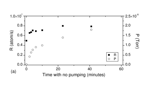
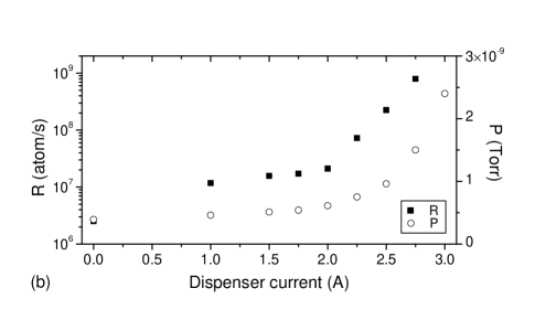
Figure 2: Response of the pressure gauge reading $P$ and the MOT loading rate $R$ to (a) turning off the chamber pumps and (b) increasing the Rb dispenser current.

Another way to vary the pressure is to operate the Rb dispensers. Figure 2(b) shows the response as a function of current, after allowing the system to equilibrate for 40 minutes after each change. Here the relative change in $P$ is small compared to the change in $R$. This is perhaps surprising, since the ionization gauge sensitivity to Rb is quite high, about twenty times larger than the sensitivity to H₂ Summers (1966). Also, both the measurements of MOT loss rates described below and the observation of Rb vapor fluorescence indicate that when the dispenser is running at higher currents, Rb is the dominant gas species present. It might therefore be expected that the gauge reading would scale with the loading rate.

We interpret the lack of such scaling to mean that Rb atoms are predominantly gettered by the chamber walls before reaching the gauge. At low surface coverage, the binding energy between alkali atoms and metal substrates is of order 3 eV Aruga and Murata (1989), and binding energies to glass are expected to be similar Garofalini and Zirl (1988). The vapor pressure resulting from such bonds will be negligible at room temperature. Rubidium will also react chemically with water and other surface contaminants. It is thus plausible that the probability for Rb atoms to make their way from the MOT region to the gauge is relatively low.

Of course, the gettering effect will become saturated as Rb coverage builds up. For the dispenser emission rates used here, it would require hours or days to deposit one monolayer of Rb over the entire surface area of the MOT chamber. Because we operate the dispensers only for a few hours per day on average, the ion pump can be expected to maintain the chamber surfaces in a mostly clean state where gettering is effective.

We tested the surface gettering interpretation by running a dispenser that was attached to a pumping station with a residual gas analyzer. Conductance from the dispenser to the analyzer was about 0.3 L/s and from the analyzer to the pump was 15 L/s. The dispenser was run until Rb metal was observably deposited on a glass surface, indicating a partial pressure comparable to the vapor pressure of bulk Rb, $4\times 10^{-7}$ Torr. No Rb peaks were observed at the analyzer, with a sensitivity of $1\times 10^{-13}$ Torr. This indicates an effective pumping speed for Rb of at least $10^{6}$ L/s, which would seem to require pumping action by the chamber walls.

This explanation implies that the total vacuum pressures measured at the gauge and at the MOT location can be significantly different, raising the question of exactly which pressure is to be determined with our technique. We believe that, in practice, it is the pressure coming from non-Rb species that is of greatest interest to a vacuum system designer. Most systems will anyway provide a way to control the partial pressure of the species being studied, meaning that the loading and loss rates for that species can be optimized for the application at hand whether a pressure gauge is available or not. A gauge is instead typically used for diagnosing problems such as vacuum leaks, contaminated surfaces, or insufficient pump capacity, all of which impact the background gas pressure. We therefore focus on the pressure $P$ as measured by the ionization gauge, and treat $P$ and $R$ as effectively independent variables in our analysis. (This now justifies our neglect in Section II of excited state collisions between identical atoms.)

Figure 3(a) shows how the MOT loss rate $\Gamma$ varied with pressure after our ion pumps were turned off as in Fig. 2(a). The clearly linear relationship can be described by $\Gamma=\Gamma_{0}^{\prime}+bP$, as expected. When the dispensers are activated, the loss rate increases further, as seen in Fig. 3(b). The solid line is a linear fit to the form $\Gamma-bP=\Gamma_{0}+aR$, indicating a relationship

$$\Gamma=\Gamma_{0}+aR+bP$$ (11)

as seen in Fig. 3(c). In relation to (3), here $\Gamma_{0}$ accounts for two-body losses $\beta\bar{n}$, $b$ accounts for collisional losses due to background gases, and $a$ accounts for collisional losses due to hot Rb atoms. If $\bar{n}$ varies with $R$, the $aR$ term would also include that variation to first order.

Fitting both data sets together yields values $\Gamma_{0}=0.036(9)$ s^-1, $a=8.5(1)\times 10^{-10}$, and $b=2.9(2)\times 10^{7}$ Torr^-1 s^-1. The error values listed represent the fit uncertainty, estimated from the parameter variation required to increase $\chi^{2}=\sum(\Gamma-\Gamma_{\mbox{\scriptsize fit}})^{2}$ by a factor of two from its minimum value. In particular, we note that the $b$ parameter is in reasonable agreement with the theoretical calculation of Section 2.

Figure 3: Dependence of the MOT loss rate $\Gamma$ on the load rate $R$ and gauge pressure $P$. (a) Response to turning off the chamber pumps as in Fig. 2(a). The line is a linear fit. (b) Response to increasing the dispenser current as in Fig. 2(b). The curve is a linear fit. (c) Comparison between the measured loss rate $\Gamma$ and the model loss rate $\Gamma_{\mbox{\scriptsize fit}}=\Gamma_{0}+aR+bP$, for fit parameters $\Gamma_{0}=0.036$ s^-1, $a=8.55\times 10^{-10}$, and $b=2.9\times 10^{7}$ Torr^-1s^-1. The line shows $\Gamma=\Gamma_{\mbox{\scriptsize fit}}$.

The data of Fig. 3 were all taken under identical conditions for the MOT, with an intensity of 40 mW/cm² and a detuning of -17 MHz. Figures 4 and 5 show how the loss coefficients vary under changes in the intensity, detuning, and choice of isotope. In most cases, the data are dominated by large loss rate values and the fits give $\Gamma_{0}$ consistent with zero. The observed loss rates at low $R$ and $P$ ranged from 0.01 to 0.1 s^-1 for ⁸⁷Rb and 0.1 to 0.2 s^-1 for ⁸⁵Rb.

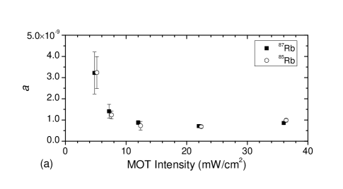
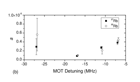
Figure 4: Loss parameter $a=\partial\Gamma/\partial R$ as a function of (a) total intensity and (b) detuning, for each Rb isotope. Points for the two isotopes are offset slightly for clarity.

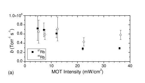
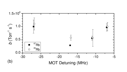
Figure 5: Loss parameter $b=\partial\Gamma/\partial P$ as a function of (a) total intensity and (b) detuning, for each Rb isotope. Points for the two isotopes are offset slightly for clarity.

It is reasonable that $a$ should diverge as the laser intensity approaches zero, because the load rate $R$ will vanish even if $\gamma_{\mbox{\scriptsize Rb}}$ remains constant. Figure 4(a) exhibits this behavior, but otherwise the variation in $a$ and $b$ is modest, as expected from the analysis of Section II. In particular, the variation in $b$ by roughly a factor of two over a large range of MOT parameters supports its utility for pressure estimation. An error-weighted average of all the data gives $b=5(2)\times 10^{7}$ Torr^-1 s^-1 where the uncertainty is taken as the standard deviation of the values. In terms of the loading time $\tau=1/\Gamma$, we have $P\approx 2\times 10^{-8}$ Torr s/$\tau$.

We also checked the dependence of $b$ on beam diameter and magnetic field gradient. We observed no change in the trap loading time for beam diameters as small as 1.5 cm, or for magnetic field gradients in the range of 5 to 10 G/cm.

To confirm the reliability of the loss-pressure calibration, we performed similar measurements in two other laser cooling apparatuses. The first featured a vacuum system similar to the one detailed above, but with independent lasers and optics, larger laser beams, a Varian ion pump in place of the Duniway model, and a different ionization gauge controller. Under its normal operating conditions with ⁸⁷Rb, this system gave $b=5(1)\times 10^{-7}$ Torr^-1 s^-1, in good agreement with the measurements in the original chamber. Here the measured value of $\Gamma_{0}$ was 0.12 s^-1.

The second alternate system belonged to another research group and was considerably different. Here a ⁸⁵Rb MOT was formed in a 15-cm diameter, 10-cm wide cylindrical stainless steel chamber with glass windows. It was pumped by a 15 L/s Gamma Vacuum ion pump. The pump and an ionization gauge were attached to the chamber through a conflat cross with an estimated conductance of 40 L/s for each. A single rubidium dispenser was mounted on a second, similar, cross. This MOT used three retro-reflected cooling beams. Under normal operating conditions, the system gave $b=6(2)\times 10^{7}$ Torr^-1 s^-1, again in good agreement with our other results. At low $R$ and $P$, we found $\Gamma_{0}=0.3$ s^-1.

IV Discussion

The preceding theoretical and experimental observations lead to the conclusion that measurements of MOT loading times can indeed provide a useful indicator of vacuum pressure. In practice, measurements should be made at low load rates so that $aR$ is negligible. The pressure sensitivity will then be limited by the two-body loss term $\Gamma_{0}$: if $bP$ is small compared to $\Gamma_{0}$, then the loading time will be nearly independent of the pressure.

In principle, $\Gamma_{0}=\beta\bar{n}$ can be determined and subtracted from the total loss rate to increase the pressure sensitivity. Experimental and theoretical estimates for $\beta$ are available Gensemer et al. (1997), and $\bar{n}$ can be measured. Unfortunately, accurate density measurements are difficult, and $\beta$ does depend significantly on the MOT parameters. Gensemer et al. report $\beta\approx 10^{-11}$ cm³ s^-1 for both Rb isotopes at an intensity of 40 mW/cm² and detuning of -17 MHz Gensemer et al. (1997). Estimating our density at $10^{10}$ cm^-3 gives $\beta\bar{n}=0.1$, compared to our observations of $\Gamma_{0}=0.04$ s^-1 for ⁸⁷Rb and 0.1 for ⁸⁵Rb. We also observe the $\Gamma_{0}$ rate to vary significantly with beam alignment, presumably due to variations in the density.

This issue can be circumvented in experiments with a MOT that is loaded from a beam, or by another method that can be rapidly turned off. In this case, the MOT can be filled, the loading turned off, and the subsequent decay observed. Intra-trap collisions may cause the decay to be non-exponential at first, but as the density is reduced an exponential regime is reached where losses are dominated by background collisions. If this regime can be observed, the background loss rate can be determined directly. This technique was used, for instance, by Prentiss et al. Prentiss et al. (1988).

In a typical vapor-loaded MOT such measurements are not possible, so extending the pressure sensitivity below the limit set by $\Gamma_{0}$ will be difficult. Nonetheless, we observed $\Gamma_{0}$ as low as 0.013 s^-1 for ⁸⁷Rb using a total intensity of 4 mW/cm², a detuning of -17 MHz, and carefully aligned and power-balanced beams. This corresponds to a pressure limit of $2.5\times 10^{-10}$ Torr, which is less sensitive than possible with an ionization gauge, but better than typically achieved with an ion pump. This also corresponds to our system’s base pressure, suggesting that the loss rate is still pressure limited here. Similar MOT loss rates have been observed by other groups for all the alkali atoms Raab et al. (1987); Prentiss et al. (1988); Sesko et al. (1991); Kawanaka et al. (1993); Myatt et al. (1996); Williamson III (1997); Gensemer et al. (1997), with background pressures (when reported) of $2\times 10^{-10}$ Torr or lower, as expected. The lowest reported MOT loss rate we are aware of is about 1 hour^-1 for a cesium MOT in a cryogenic chamber Willems and Libbrecht (1995). This corresponds to a room temperature pressure of $5\times 10^{-12}$ Torr, exceeding the sensitivity of most commercial ionization gauges.

In practice it would be difficult to know whether an observed loading time was in fact limited by pressure or by pressure-independent losses. For instance, one of the alternate systems we measured had $\Gamma_{0}=0.3$ s^-1, indicating a pressure of $6\times 10^{-9}$ Torr. This substantially exceeds the measured pressure $1\times 10^{-9}$ Torr, presumably due to a large inelastic collision loss rate for the the laser parameters and beam alignment used in that system. Without a pressure gauge, however, it would only be possible to say that the pressure was at most $6\times 10^{-9}$ Torr. Given the difficulty in predicting $\Gamma_{0}$ for a given system, the absolute sensitivity of the MOT technique is difficult to quantify. It would seem, however, that if care is taken to adjust the MOT parameters to make $\Gamma_{0}$ as small as possible, sensitivities in the $10^{-10}$ Torr range are achievable.

At the other extreme, the technique will fail at high pressures when it is not possible to achieve a MOT. This would be particularly pernicious when it is not clear whether the lack of a MOT is due to poor vacuum or to some other problem. At high dispenser currents, we observed MOTs with $\Gamma$ up to 20 s^-1. Losses here were clearly dominated by collisions with hot Rb atoms, but the corresponding background pressure $\Gamma/b$ is $P=4\times 10^{-7}$ Torr. The largest background pressure we obtained by leaving the pumps turned off was $1\times 10^{-7}$ Torr, at which point the MOT still functioned.

In summary, we hope to have illustrated here that MOT loading times can provide a reasonably reliable and accurate measurement of background pressure in a UHV system. The procedure is relatively straightforward: With the MOT loading rate $R$ as small as possible, adjust the lasers and other MOT parameters to make the loading time $\tau=1/\Gamma$ as large as possible. The vacuum pressure is then at most $(b\tau)^{-1}=(2\times 10^{-8}$ Torr s)/$\tau$, roughly independent of the MOT laser parameters, background gas species, or trapped alkali species. We expect this technique to be useful in situations where a conventional pressure gauge is impractical due to other constraints on the vacuum system design.