Properties of $c_{2}$ invariants of Feynman graphs

Abstract.

The $c_{2}$ invariant of a Feynman graph is an arithmetic invariant which detects many properties of the corresponding Feynman integral. In this paper, we define the $c_{2}$ invariant in momentum space and prove that it equals the $c_{2}$ invariant in parametric space for overall log-divergent graphs. Then we show that the $c_{2}$ invariant of a graph vanishes whenever it contains subdivergences. Finally, we investigate how the $c_{2}$ invariant relates to identities such as the four-term relation in knot theory.

1. Introduction

Let $G$ be a connected graph. The graph polynomial of $G$ is defined by associating a variable $x_{e}$ to every edge $e$ of $G$ and setting

(1) $$\Psi_{G}(x)=\sum_{T\,\rm span.\,tree}\;\prod_{e\not\in T}x_{e},$$

where the sum is over all spanning trees $T$ of $G$. These polynomials first appeared in Kirchhoff’s work on currents in electrical networks [16].

Let $N_{G}$ denote the number of edges of $G$, and let $h_{G}$ denote the number of independent cycles in $G$ (the first Betti number). Of particular interest is the case when $G$ is primitive and overall logarithmically divergent:

(2) $$N_{G} = 2h_{G}$$

$$N_{\gamma} > 2h_{\gamma}\quad\hbox{ for all strict non-trivial subgraphs }\gamma\subsetneq G\ .$$

For such graphs, the corresponding Feynman integral (or residue) is independent of the choice of renormalization scheme and can be defined by the following convergent integral in parametric space ([4], [23])

(3) $$I_{G}=\int_{0}^{\infty}\cdots\int_{0}^{\infty}\frac{dx_{1}\cdots dx_{N_{G}}}{\Psi_{G}(x)^{2}}\,\delta(\sum_{i=1}^{N_{G}}x_{i}-1).$$

The numbers $I_{G}$ are notoriously difficult to calculate, and have been investigated intensively from the numerical [5, 20] and algebro-geometric points of view [4, 9]. For graphs in $\phi^{4}$ theory with subdivergences, the renormalised amplitudes can also be written in terms of graph polynomials by subtracting counter-terms from the same leading term $\Psi^{-2}_{G}(x)$ [10].

Given the difficulty in computing $I_{G}$, one seeks more efficient ways to extract qualitative information about the Feynman integral indirectly. The motivic philosophy suggests studying the graph hypersurface:

$$\overline{X}_{G}\subset{\mathbb{P}}^{N_{G}-1}$$

defined by the zero locus of the graph polynomial $\Psi_{G}$ in projective space (with no restriction on the numbers of edges or cycles in $G$). In particular, motivated by a conjecture of Kontsevich [17] (disproved for general graphs in [3]), one can consider the point counting function

$$q\mapsto|\overline{X}_{G}({\mathbb{F}}_{q})|$$

where $q=p^{n}$ is a prime power, and ${\mathbb{F}}_{q}$ is the finite field with $q$ elements. In [11], it was shown that for graphs with at least three vertices there is a map

$$c_{2}:\{\hbox{graphs with }\geq 3\hbox{ vertices}\}\rightarrow\prod_{{\rm prime\,powers}\,q}{\mathbb{Z}}/q{\mathbb{Z}}$$

such that, writing $[X_{G}]_{q}:=|X_{G}({\mathbb{F}}_{q})|,$ we have

(4) $$[X_{G}]_{q}\equiv c_{2}(G)_{q}\,q^{2}\mod q^{3}$$

where $X_{G}\subset{\mathbb{A}}^{N_{G}}$ is the affine graph hypersurface given by the zero locus of $\Psi_{G}$, and $c_{2}(G)_{q}$ is itself the point counting function on a related hypersurface. One of the motivations for studying the $c_{2}$ invariant is the following conjecture, verified for all graphs with $\leq 14$ edges, which states that it only depends on the residue of $G$ whenever it is defined.

Conjecture 1.

If $I_{G_{1}}=I_{G_{2}}$ for two primitive log-divergent graphs $G_{1}$, $G_{2}$ (i.e. which satisfy $(\ref{defnprimdiv})$) then $c_{2}(G_{1})=c_{2}(G_{2})$.

Furthermore, for graphs $G$ which evaluate to multiple zeta values, we expect the residue $I_{G}$ to drop in transcendental weight if and only if $c_{2}(G)_{q}$ is identically zero [13]. All $c_{2}$ invariants of primitive log-divergent graphs with $\leq 20$ edges are listed for the first six primes in [12].

1.1. Avatars of the $c_{2}$ invariant

Before stating our main results, it will be helpful to discuss various different incarnations of the $c_{2}$ invariant.

1. Geometric. If $k$ is a field, we can consider the class $[X_{G}]$ of the affine graph hypersurface in the Grothendieck ring of varieties $K_{0}(\mathrm{Var}_{k})$ over $k$. Let $\mathbb{L}=[{\mathbb{A}}^{1}_{k}]\in K_{0}(\mathrm{Var}_{k})$ be the equivalence class of the affine line. Whenever $G$ has at least three vertices, in other words whenever $N_{G}\geq h_{G}+2$, it was shown in [11] that there exists an element

(5) $$c_{2}(G)\in K_{0}(\mathrm{Var}_{k})/\mathbb{L}\ ,$$

given explicitly by the class of a certain hypersurface, such that

(6) $$[X_{G}]\equiv c_{2}(G)\mathbb{L}^{2}\mod\mathbb{L}^{3}\ .$$

This is a refined version of equation $(\ref{c2modq2})$.

2. Arithmetic. For some applications, and for numerical computations, it is often simpler to restrict the point counting function to the fields ${\mathbb{F}}_{p}$ of prime order only. Thus in [11] we considered the vector

(7) $$\widetilde{c}_{2}(G)=(c_{2}(G)_{2},c_{2}(G)_{3},c_{2}(G)_{5},\ldots)\in\prod_{p\,prime}{\mathbb{Z}}/p{\mathbb{Z}}\ .$$

It clearly factors through the class $(\ref{c2geom})$, but in many cases we are not able to lift computations of $\widetilde{c}_{2}(G)$ to the Grothendieck ring. In [11] we gave examples of graphs such that $\widetilde{c}_{2}(G)$ is given by the Fourier coefficients of a modular form, giving explicit counter examples to Kontsevich’s conjecture. Several more modular $\widetilde{c}_{2}$ invariants were found in [12].

3. Analytic. It turns out that for a large class of graphs, one can in principle compute the residue $I_{G}$ by integrating in parametric space [9]. After integrating out a subset of edge variables $x_{1},\ldots,x_{n}$ in $(\ref{2})$, one typically obtains an expression whose numerator is an iterated integral in the sense of K. T. Chen [14], and whose denominator is a polynomial

$$D^{n}_{G}(x_{1},\ldots,x_{n})\in{\mathbb{Z}}[x_{n+1},\ldots,x_{N_{G}}]$$

of degree at most two in each variable. When $D^{n}_{G}$ factorizes, one can define $D^{n+1}_{G}$ to be the resultant of its factors with respect to $x_{n+1}$. This sequence of polynomials (which terminates when $D^{n}_{G}$ can no longer be reduced) is called the denominator reduction. When $D^{n}_{G}$ exists, we showed in [11] that

(8) $$c_{2}(G)_{q}\equiv(-1)^{n}[D^{n}_{G}]_{q}\mod q$$

when $2h\leq N_{G}$ and $5\leq n<N_{G}$, as a consequence of the Chevalley-Warning theorem. This gives an effective way to compute $c_{2}(G)_{q}$ and is the main method for proving properties of the $c_{2}$ invariant.

4. Motivic. We expect the $c_{2}$ invariant to relate to the framing of the graph motive [4] given by the Feynman differential form (the integrand of $(\ref{2})$). This partly justifies conjecture 1 and the incarnations 1,2,3 above.

Hereafter, we shall loosely refer to the $c_{2}$ invariant as any of the variants $1-3$ above, since our results relate to all three different versions. As a result, there is considerable interplay between geometric, combinatorial, and arithmetic arguments throughout this paper.

1.2. Results

It will be convenient to make the following definition.

Definition 2.

Let $X$ be a scheme of finite type over $\mathrm{Spec}\,{\mathbb{Z}}$. Let $n\geq 0$. We say that $X$ has a $c_{n}$ invariant if $[X]_{q}\equiv 0\mod q^{n}$ for all prime powers $q$. In this case, define the $c_{n}$ invariant of $X$ to be the function:

$$c_{n}(X)\equiv[X]_{q}/q^{n}\mod q$$

from the set of prime powers $q$ to ${\mathbb{Z}}/q{\mathbb{Z}}$.

Our results are of three different types.

1.2.1. A $c_{2}$ invariant in momentum space

Our first goal is to show that the $c_{2}$ invariant is intrinsic and is not simply a feature of the choice of integral representation for the Feynman graph. For this, we define a momentum space representation for the $c_{2}$ invariant as follows.

The Feynman integral in momentum space is the integral of an algebraic differential form with singularities along a union of quadrics $Q_{1},\ldots,Q_{N_{G}}$. With an appropriate choice of space-time metric, we show that the scheme $V(Q_{1}\ldots Q_{N_{G}})$, which is defined over ${\mathbb{Z}}$, has a $c_{2}$ invariant in the sense of definition 2, and we define $c_{2}^{\rm mom}(G)$ to be $c_{2}(V(Q_{1}\ldots Q_{N_{G}}))$. In other words, we have the equation:

$$c_{2}(G)^{\rm mom}_{q}\equiv[Q_{1}Q_{2}\cdots Q_{N_{G}}]_{q}/q^{2}\mod q.$$

The first result is that the $c_{2}$ invariant in momentum space is the same as the $c_{2}$ invariant in parametric space for logarithmically divergent graphs.

Theorem 3.

Let $G$ be a graph with $h_{G}\geq 3$. If $2h_{G}=N_{G}$ then

$$c_{2}(G)^{\rm mom}_{q}\equiv c_{2}(G)_{q}\mod q.$$

The proof requires studying the singular locus ${\rm Sing}(X_{G})$ of $X_{G}$, and in particular proving the following intermediate result.

Theorem 4.

If $G$ has at least 3 vertices, then ${\rm Sing}(X_{G})$ has a $c_{1}$ invariant.

This suggests studying the $c_{n}$ invariants of the singular locus of $X_{G}$ in its own right. In fact, we believe that the $c_{1}$ invariant of ${\rm Sing}(X_{G})$ should vanish, in which case one could define its $c_{2}$ invariant, which we expect to be non-zero in general. This would give a new graph invariant $c^{\mathrm{sing}}_{2}(G)=c_{2}({\rm Sing}\,X_{G})$, which would be interesting to understand combinatorially.

1.2.2. Vanishing for subdivergences

The second set of results extends our previous work on criteria for graphs to have weight drop [13].

Theorem 5.

Let $G$ be an overall logarithmically divergent graph in $\phi^{4}$ theory. If $G$ has a non-trivial divergent subgraph then $c_{2}(G)_{q}=0$.

Such a graph $G$ with a subdivergence can always be written as a $2,3$, or $4$-edge join. In the first two cases, we prove that $c_{2}(G)$ vanishes in the Grothendieck ring, but the case of a $4$-edge join is more subtle and we can only show the result on the level of point counting functions. If reduced denominators $D^{n}_{G}$ exist for the elimination of all edges of the subdivergence, then in the last non-trivial step $D^{n}_{G}$ equals the square of the graph polynomial of $G$ with fully contracted subdivergence. This explains the vanishing of the $c_{2}$ invariant on the level of denominator reduction.

Given the expected relation between vanishing $c_{2}$ and transcendental weight drop of Feynman amplitudes, theorem 5 is evidence for a folklore conjecture which states that the highest weight part of the lowest logarithmic power of the renormalised amplitudes in $\phi^{4}$ theory is independent of the choice of renormalisation scheme.

1.2.3. Combinatorial identities

In the light of conjecture 1, and the many observed but unexplained algebraic relations between residues of Feynman graphs, an important question is to understand precisely which combinatorial information is contained in the $c_{2}$ or related invariants.

For a list of currently known or conjectured properties of the $c_{2}$ invariant, see [11], §4. To these can be added some further relations for the denominator reduction described in [13], §4.4-4.7, which immediately imply identities for the $c_{2}$ invariant via $(\ref{introDn2c2})$. Although an overarching combinatorial explanation for all these identities is still lacking, in $\S 6$ we describe some new additive properties of denominator polynomials which give a single explanation for many of the identities of [13].

Finally, there remains the question of trying to relate $c_{2}(G)$ to other classical invariants in the theory of graphs. A tantalizing but mysterious connection between knots and Feynman integrals was investigated by Broadhurst and Kreimer in the 90’s [5, 7, 8, 18], but has proven very hard to verify in concrete cases because of the difficulty in computation of Feynman integrals, and the high loop orders of the diagrams involved. The $c_{2}$ invariant provides us with a tool to investigate such identities without having to compute any integrals.

In this paper, we investigated the 4-term relation for chord diagrams, which was shown to hold in some cases in [6], but found no such relation on the level of $c_{2}$ invariants in $\phi^{4}$ theory. To our surprise, however, we found that the 4-term identity actually holds true on the level of the denominator polynomials $D^{7}_{G}$.

2. Reminders on graph polynomials

For the convenience of the reader, we gather some of the results on graph polynomials and various auxiliary polynomials to be used later.

2.1. Graph matrix

Let $G$ be any graph. We will use the following matrix representation for the graph polynomial.

Definition 6.

Choose an orientation on the edges of $G$, and for every edge $e$ and vertex $v$ of $G$, define the incidence matrix:

$$(\mathcal{E}_{G})_{e,v}=\left\{\begin{array}[]{rl}1,&\hbox{if the edge }e\hbox{ begins at }v\hbox{ and does not end at }v,\\ -1,&\hbox{if the edge }e\hbox{ ends at }v\hbox{ and does not begin at }v,\\ 0,&\hbox{otherwise}.\end{array}\right.$$

Let $A$ be the diagonal matrix with entries $x_{e}$, for $e\in E(G)$, and set

$$\widetilde{M}_{G}=\left(\begin{array}[]{c|c}A&\mathcal{E}_{G}\\ \hline\cr{-}\mathcal{E}_{G}^{T}&0\\ \end{array}\right)$$

where the first $N_{G}$ rows and columns are indexed by the set of edges of $G$, and the remaining $v_{G}$ rows and columns are indexed by the set of vertices of $G$, in some order. The matrix $\widetilde{M}_{G}$ has corank $\geq 1$. Choose any vertex of $G$ and let $M_{G}$ denote the square $(N_{G}+v_{G}-1)\times(N_{G}+v_{G}-1)$ matrix obtained from it by deleting the row and column indexed by this vertex.

It follows from the matrix-tree theorem that the graph polynomial satisfies

$$\Psi_{G}=\det(M_{G})\ .$$

This formula implies that $\Psi_{G}$ vanishes if $G$ has more than one component.

2.2. Dodgson polynomials

We use the following notation.

Definition 7.

If $f=f_{1}+f^{1}x_{1}$ and $g=g_{1}+g^{1}x_{1}$ are polynomials of degree one in $x_{1}$, recall that their resultant is defined by:

(9) $$[f,g]_{x_{1}}=f^{1}g_{1}-f_{1}g^{1}\ .$$

Definition 8.

Let $I,J,K$ be subsets of the set of edges of $G$ which satisfy $|I|=|J|$. Let $M_{G}(I,J)_{K}$ denote the matrix obtained from $M_{G}$ by removing the rows indexed by the set $I$ and columns indexed by the set $J$, and setting $x_{e}=0$ for all $e\in K$. Let

(10) $$\Psi_{G,K}^{I,J}=\det M_{G}(I,J)_{K}\ .$$

We write $\Psi^{I}_{G,K}$ as a shorthand for $\Psi^{I,I}_{G,K}$ and drop the subscript $K$ if it is empty. Since the matrix $M_{G}$ depends on various choices, the polynomials $\Psi^{I,J}_{G,K}$ are only well-defined up to sign. In what follows, for any graph $G$, we shall fix a particular matrix $M_{G}$ and this will fix all the signs in the polynomials $\Psi^{I,J}_{G,K}$ too.

We now state some identities between Dodgson polynomials which will be used in the sequel. The proofs can be found in ([9], §2.4-2.6).

1. The contraction-deletion formula. The graph polynomial is linear in its variables and fulfills the contraction-deletion relation

   (11) $$\Psi_{G}=\Psi_{G\backslash e}x_{e}+\Psi_{G/\!\!/e}\ ,$$

   where the graph polynomial of disconnected graphs is zero. Likewise the contraction ($/\!\!/$) of a self-loop is zero in the graph algebra and $\Psi_{0}=0$. More generally, if $|I|=|J|$, we have:

   $$\Psi^{Ie,Je}_{G,K}=\pm\Psi^{I,J}_{G\backslash e,K}\,\hbox{ and }\Psi^{I,J}_{G,Ke}=\pm\Psi^{I,J}_{G/\!\!/e,K}\ .$$

2. Dodgson identities. Let $I,J$ be two subsets of edges of $G$ such that $|I|=|J|$ and let $a,b,x\notin I\cup J\cup K$ with $a,b<x$ (or $x<a,b$ ). The first identity is:

   $$\big{[}\Psi^{I,J}_{G,K},\Psi^{Ia,Jb}_{G,K}\big{]}_{x}=\Psi^{Ix,Jb}_{G,K}\Psi^{Ia,Jx}_{G,K}\ .$$

   Let $I,J$ be two subsets of edges of $G$ such that $|J|=|I|+1$ and let $a,b,x\notin I\cup J\cup K$ with $x<a<b$. Then the second identity is:

   $$\big{[}\Psi^{Ia,J}_{G,K},\Psi^{Ib,J}_{G,K}\big{]}_{x}=-\Psi^{Ix,J}_{G,K}\Psi^{Iab,Jx}_{G,K}\ .$$

3. Plücker identities. Let $i_{1}<i_{2}<i_{3}<i_{4}$. Then

   $$\Psi^{i_{1}i_{2},i_{3}i_{4}}_{G}-\Psi^{i_{1}i_{3},i_{2}i_{4}}_{G}+\Psi^{i_{1}i_{4},i_{2}i_{3}}_{G}=0\ .$$

   For an increasing sequence of edges $i_{1}<\ldots<i_{6}$ we have

   $$\Psi^{i_{1}i_{2}i_{3},i_{4}i_{5}i_{6}}_{G}-\Psi^{i_{1}i_{2}i_{4},i_{3}i_{5}i_{6}}_{G}+\Psi^{i_{1}i_{2}i_{5},i_{3}i_{4}i_{6}}_{G}-\Psi^{i_{1}i_{2}i_{6},i_{3}i_{4}i_{5}}_{G}=0\ .$$

4. Vanishing. Suppose that $E=\{e_{1},\ldots,e_{k}\}$ is the set of edges which are adjacent to a given vertex of $G$. Then $\Psi^{I,J}_{G,K}=0$ if $E\subset I$ or $E\subset J$. Now suppose that $E=\{e_{1},\ldots,e_{k}\}$ is a set of edges in $G$ which contain a cycle. Then $\Psi^{I,J}_{G,K}=0$ if $(E\subset I\cup K$ or $E\subset J\cup K)$ and $E\cap I\cap J=\emptyset$.

2.3. Spanning forest polynomials

Dodgson polynomials are in turn linear combinations of more basic polynomials, called spanning forest polynomials [13].

Definition 9.

Let $X$ be a set of vertices of $G$, and let $P=\{P_{1},\ldots,P_{k}\}$ be a partition of $X$. Define the spanning forest polynomial by

$$\Phi_{G}^{P}=\sum_{F}\prod_{e\not\in F}x_{e}$$

where the sum runs over spanning forests $F=T_{1}\cup\ldots\cup T_{k}$ where each tree $T_{i}$ (possibly a single vertex) of $F$ contains the vertices in $P_{i}$ and no other vertices of $X$. Thus $V(T_{i})\supseteq P_{i}$ and $V(T_{i})\cap P_{j}=\emptyset$ for $j\neq i$.

We represent $\Phi_{G}^{P}$ by associating a colour to each part of $P$ and drawing $G$ with the vertices in $X$ coloured accordingly.

Proposition 10.

Let $I,J$ be sets of edges of $G$ with $|I|=|J|$ and $I\cap J=\varnothing$. Then we can write

$$\Psi_{G}^{I,J}=\sum_{i}f_{i}\Phi_{G}^{P_{i}}$$

where the sum runs over partitions of $V(I\cup J)$ and $f_{i}\in\{-1,0,1\}$. In particular, $f_{i}\neq 0$ precisely when each forest consistent with $P_{i}$ becomes a tree in $G/I\backslash J$ and in $G/J\backslash I$.

Note that the sign $f_{i}$ can be computed by taking any forest $F$ consistent with $P_{i}$ and then considering the determinant of the matrix obtained from $M_{G}$ by removing rows and columns indexed by the set of edges not in $F$. This determinant reduces [13] to

(12) $$\det[E_{I}N]\det[E_{J}N]$$

where $E_{I}$ is the matrix of the columns corresponding to edge indices $I$ of $\mathcal{E}_{G}$ with one row removed, likewise for $E_{J}$, and $N$ is the matrix of columns corresponding to edges of $G\backslash(I\cup J)$ which do not appear in the forest $F$.

2.4. Denominator reduction

Definition 11.

Let $i,j,k,l,m$ be five distinct edges in $G$. The five-invariant of these edges is the polynomial defined up to a sign by the resultant

$${}^{5}\Psi_{G}(i,j,k,l,m)=\pm[\Psi^{ij,kl},\Psi^{ik,jl}]_{m}\ .$$

Permuting the order of the edges $i,j,k,l,m$ only affects the overall sign.

Denominator reduction is the name given to the elimination of variables by taking iterated resultants, starting with the 5-invariant. Let $G$ be a graph, and order its edges $1,\ldots,{N_{G}}$. Set $D^{5}_{G}(1,\ldots,5)=\pm{}^{5}\Psi_{G}(1,\ldots,5)$, and define a sequence of polynomials (conditionally) as follows.

Definition 12.

Let $n\geq 5$ and suppose that $D^{n}_{G}(1,\ldots,n)$ is defined, and further that it factorizes into a product of factors $f,g$ of degree $\leq 1$ in $x_{n+1}$. Then set

$${D}^{n+1}_{G}(1,\ldots,{n+1})=\pm[f,g]_{n+1}\ ,$$

We say that $G$ is denominator reducible if there exists an order of edges such that ${D}^{n}_{G}(1,\ldots,{n})$ is defined for all $n$. We say that $G$ has weight drop if there exists an order of edges such that ${D}^{n}_{G}(1,\ldots,{n})$ vanishes for some $n$.

The relation between the denominator reduction and $c_{2}$ invariant is given by the following theorem (theorem 29 in [11]).

Theorem 13.

Let $G$ be a connected graph with $2h_{G}\leq N_{G}$. Suppose that $D^{n}_{G}(e_{1},\ldots,e_{n})$ is the result of the denominator reduction after $5\leq n<N_{G}$ steps. Then

(13) $$c_{2}(G)_{q}\equiv(-1)^{n}[D^{n}_{G}(e_{1},\ldots,e_{n})]_{q}\mod q\ .$$

3. The $c_{2}$ invariant in momentum space

For any primitive log-divergent graph $G$, the residue $I_{G}$ of $G$ can be written as an integral in various different representations. From a physical point of view, the most natural of these is the representation of $I_{G}$ as an integral in momentum space [20]. Other possibilities are parametric space as explained in the introduction, position space, related to momentum space by a Fourier transform, and dual parametric space which is linked to the parametric formulation (3) by inversion of the Schwinger coordinates $x_{e}$. In the spirit of conjecture 1 for graphs which have a residue, all these representations should lead to equivalent $c_{2}$ invariants.

Because we work over a general field $k$ which does not necessarily contain $\sqrt{-1}$ or may have characteristic 2 the choice of metric becomes relevant for the definition of Feynman rules in momentum and in position space. Here it is best to use a twistor type metric with signature $(+,-,+,-)$. We choose the metric $\eta$ to be of the form

(14) $$\eta=\left(\begin{array}[]{cccc}0&1&0&0\\ 1&0&0&0\\ 0&0&0&1\\ 0&0&1&0\end{array}\right)$$

and write $p=(p^{+},p^{-},p^{\prime+},p^{\prime-})$. Then the propagator of a massless particle becomes $1/Q(p)$ with (see [15])

(15) $$Q(p)=p^{+}p^{-}+p^{\prime+}p^{\prime-},$$

which is linear in the coordinates. The value of the residue does not depend on the chosen metric. Physically this means that the residue is a scalar.

Likewise, in position space the propagator between $x$ and $y$ in $k^{4}$ is $1/Q(x-y)$.

In the following we focus on momentum space. We fix a basis of $h_{G}$ independent cycles in $G$ with respect to which the momenta $p=(p_{1},\ldots,p_{h_{G}})$ are routed. The graph $G$ has $N_{G}$ edges with propagators $1/Q_{1}(p),\ldots,1/Q_{N_{G}}(p)$. We will show that the ‘Schwinger trick’ lifts to the $c_{2}$ invariant proving the existence of a $c_{2}$ invariant in momentum space if $2h_{G}\geq N_{G}$ and its equivalence with (4) for log-divergent graphs.

Example 14.

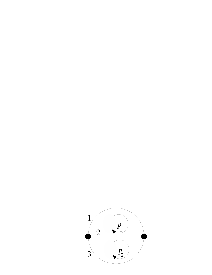
Figure 1. The sunset graph.

We consider the sunset graph in fig. 1. The edges 1,2,3 have the propagators $1/Q_{1},1/Q_{2},1/Q_{3}$ with

$$Q_{1} = p_{1}^{+}p_{1}^{-}+p_{1}^{\prime+}p_{1}^{\prime-}$$

$$Q_{2} = (p_{1}^{+}-p_{2}^{+})(p_{1}^{-}-p_{2}^{-})+(p_{1}^{\prime+}-p_{2}^{\prime+})(p_{1}^{\prime-}-p_{2}^{\prime-})$$

$$Q_{3} = p_{2}^{+}p_{2}^{-}+p_{2}^{\prime+}p_{2}^{\prime-}$$

An explicit computer calculation using Stembridge’s reduction [22] yields

$$[Q_{1}Q_{2}Q_{3}]=3\mathbb{L}^{7}-7\mathbb{L}^{5}+4\mathbb{L}^{4}+4\mathbb{L}^{3}-3\mathbb{L}^{2}.$$

The momentum space $c_{2}$ invariant exists (see proposition-definition 17 below) and is equal to the $\mathbb{L}^{2}$ coefficient of $[Q_{1}Q_{2}Q_{3}]$, namely $-3\mod\mathbb{L}$.

The key tool in the Schwinger trick is the universal quadric

(16) $${\mathcal{Q}}(x,p)=x_{1}Q_{1}(p)+x_{2}Q_{2}(p)+\ldots+x_{N_{G}}Q_{N_{G}}(p).$$

From the matrix-tree theorem used in the Schwinger trick [15] we conclude that there exists a symmetric $h_{G}\times h_{G}$ matrix $N$ such that

(21) $${\mathcal{Q}}(x,p) = (p^{-},p^{\prime-})\left(\begin{array}[]{cc}N(x)&0\\ 0&N(x)\end{array}\right)\left(\begin{array}[]{c}p^{+}\\ p^{\prime+}\end{array}\right),\quad\hbox{with}$$

(22) $$\hbox{det}\,N(x) = \Psi_{G}(x).$$

Here $p^{\pm}=(p^{\pm}_{1},\ldots,p^{\pm}_{h_{G}})$ and likewise $p^{\prime\pm}$.

Proposition 15.

1. The singular locus of $X_{G}$ is given by

   (23) $${\rm Sing}(X_{G})=\{x:{\rm rank\,}N(x)<h_{G}-1\}.$$

2. Let $I\subseteq\{1,\ldots,N_{G}\}$ and $N_{\bar{I}}(x)=N(x)|_{x_{k}=0,\,{\rm if}\,k\not\in I}$ be obtained from $N$ by setting all variables to zero whose index is not in $I$. Then

   (24) $$(\mathbb{L}-1)\mathbb{L}^{|I|-1}[Q_{i,i\in I}]=(\mathbb{L}-1)\mathbb{L}^{2h_{G}-1}[N_{\bar{I}}\cdot p^{+},N_{\bar{I}}\cdot p^{\prime+}].$$

3. With $\Psi_{G,{\bar{I}}}(x)=\Psi_{G}(x)|_{x_{k}=0,\,{\rm if}\,k\not\in I}$ we have

   (25) $$[N_{\bar{I}}\cdot p^{+},N_{\bar{I}}\cdot p^{\prime+}]\equiv(\mathbb{L}^{2}-1)[\Psi_{G,{\bar{I}}}]-\mathbb{L}^{2}[{\rm rank\,}N_{\bar{I}}<h_{G}-1]+\mathbb{L}^{|I|}\!\mod\mathbb{L}^{4}.$$

Proof.

1. With elementary row and column transformations (which correspond to a change of cycle basis) we can transform $N$ into a matrix $\tilde{N}$ with the property that in each diagonal entry $\tilde{N}_{i,i}$ there exists a variable (say $x_{i}$) which does not occur in any other entry of $\tilde{N}$. Because elementary row and column transformations preserve the rank of the matrix we may assume without restriction that $N=\tilde{N}$. Let $x\in\hbox{Sing}\,(X_{G})$. We thus have $\partial_{x_{i}}\Psi_{G}(x)=\det N^{i,i}(x)=0$ for $i=1,\ldots,h_{G}$ where $N^{J,K}$ is the matrix $N$ with rows $J$ and columns $K$ deleted. We have $\det N(x)=0$, and the Dodgson identity for the symmetric matrix $N$:

   $$(\det N^{i,j})^{2}=\det N^{i,i}\det N^{j,j}-\det N\det N^{ij,ij},$$

   implies $\det N(x)^{i,j}=0$ for all $i,j=1,\ldots,h_{G}$. Hence ${\rm rank\,}N<h_{G}-1$.

   On the other hand, if ${\rm rank\,}N(x)<h_{G}-1$ then $\det N(x)^{i,j}=0$ for all $i,j=1,\ldots h_{G}$, and in particular $\partial_{x_{i}}\Psi_{G}(x)=\det N^{i,i}(x)=0$ for $i=1,\ldots,h_{G}$. Hence $x\in{\rm Sing}(X_{G})$ and (23) is established.

2. Consider the universal quadric ${\mathcal{Q}}_{I}=\sum_{i\in I}x_{i}Q_{i}$ and calculate its class in the Grothendieck ring in two different ways.

   Firstly, ${\mathcal{Q}}_{I}$ defines a family of hyperplanes in the $|I|$ dimensional affine space ${\mathbb{A}}^{|I|}$ with coordinates $x_{i}$. Consider the fiber of the projection $V({\mathcal{Q}}_{I})\rightarrow{\mathbb{A}}^{4h_{G}}$. In the generic case it is a hyperplane in ${\mathbb{A}}^{|I|}$ whose class is $\mathbb{L}^{|I|-1}$. Otherwise, all $Q_{i},i\in I$ vanish and the fiber is ${\mathbb{A}}^{|I|}$. We have

   $$[{\mathcal{Q}}_{I}]=\mathbb{L}^{|I|-1}(\mathbb{L}^{4h_{G}}-[Q_{i,i\in I}])+\mathbb{L}^{|I|}[Q_{i,i\in I}].$$

   Secondly, from (21) we have

   $${\mathcal{Q}}_{I}(x,p)=(p^{-},p^{\prime-})\left(\begin{array}[]{cc}N_{\bar{I}}(x)&0\\ 0&N_{\bar{I}}(x)\end{array}\right)\left(\begin{array}[]{c}p^{+}\\ p^{\prime+}\end{array}\right)$$

   and so ${\mathcal{Q}}_{I}$ also defines a family of hyperplanes in the $p^{-}$ variables. We now consider the fiber of the projection $V({\mathcal{Q}}_{I})\rightarrow{\mathbb{A}}^{|I|+2h_{G}}$ and obtain

   $$[{\mathcal{Q}}_{I}]=\mathbb{L}^{2h_{G}-1}(\mathbb{L}^{|I|+2h_{G}}-[N_{\bar{I}}\cdot p^{+},N_{\bar{I}}\cdot p^{\prime+}])+\mathbb{L}^{2h_{G}}[N_{\bar{I}}\cdot p^{+},N_{\bar{I}}\cdot p^{\prime+}].$$

   Together we obtain (24).

3. The equations $N_{\bar{I}}\cdot p^{+},N_{\bar{I}}\cdot p^{\prime+}$ form two identical systems of $h_{G}$ linear equations in the variables $p^{+}$ and $p^{\prime+}$, respectively. The vanishing locus of each system is ${\mathbb{A}}^{n}$ where $n={\rm corank\,}(N_{\bar{I}})$. Hence

   $$[N_{\bar{I}}\cdot p^{+},N_{\bar{I}}\cdot p^{\prime+}] \equiv [{\rm corank\,}N_{\bar{I}}=0]+\mathbb{L}^{2}[{\rm corank\,}N_{\bar{I}}=1]\mod\mathbb{L}^{4}$$

   $$\equiv \mathbb{L}^{|I|}-[{\rm corank\,}N_{\bar{I}}>0]$$

   $$+\,\mathbb{L}^{2}([{\rm corank\,}N_{\bar{I}}>0]-[{\rm corank\,}N_{\bar{I}}>1])\mod\mathbb{L}^{4}$$

   Because ${\rm corank\,}N_{\bar{I}}>0\Leftrightarrow\Psi_{G,{\bar{I}}}=0$ we obtain (25).

∎

To progress further we pass to finite fields. Let $q=p^{n}$ be a prime power. Given polynomials $P_{1},\ldots,P_{\ell}\in{\mathbb{Z}}[x_{1},\ldots,x_{N}]$, let

$$[P_{1},\ldots,P_{\ell}]_{q}\in\mathbb{N}\cup\{0\}$$

denote the number of points on the affine variety $V(\overline{P_{1}},\ldots,\overline{P_{\ell}})\subset{\mathbb{F}}_{q}^{N}$, where $\overline{P}_{i}$ denotes the reduction of $P_{i}$ modulo $p$. The point-counting is compatible with inclusion-exclusion and Cartesian products and therefore factors through the Grothendieck ring mapping $\mathbb{L}$ to $q$.

We are interested in the point-count of the zero locus of the denominator of the momentum space differential form which is $[Q_{1}Q_{2}\cdots Q_{N_{G}}]_{q}$.

Proposition 16.

Let $h_{G}\geq 2$, $2h_{G}\geq N_{G}$ and $E$ be the edge-set of $G$, then

(26) $$[Q_{1}Q_{2}\cdots Q_{N_{G}}]_{q} \equiv (-q)^{2h_{G}-N_{G}}\Big{[}[\Psi_{G}]_{q}+q^{2}[{\rm Sing}(X_{G})]_{q}$$

$$-\,q\sum_{e\in E}[\Psi_{G/\!\!/e}]_{q}+q^{2}\sum_{e_{1},e_{2}\in E}[\Psi_{G/\!\!/e_{1}e_{2}}]_{q}\Big{]}\mod q^{3}.$$

Proof.

By inclusion exclusion we obtain

$$[Q_{1}Q_{2}\cdots Q_{N_{G}}]_{q}=\sum_{\emptyset\neq I\subseteq\{1,\ldots,N_{G}\}}(-1)^{|I|-1}[Q_{i,i\in I}]_{q}.$$

By prop. 15 (2) we have $[Q_{i,i\in I}]_{q}=q^{2h_{G}-|I|}[N_{\bar{I}}\cdot p^{+},N_{\bar{I}}\cdot p^{\prime+}]_{q}$. Next, we use prop. 15 (3). For $2h_{G}\geq N_{G}$ the second term on the right hand side of (25) survives mod $q^{3}$ only in the case $I=\{1,\ldots,N_{G}\}$ where it gives $-q^{2}[{\rm Sing}(X_{G})]_{q}$ by prop. 15 (1). The third term on the right hand side of (25) is multiplied by $q^{2h_{G}-|I|}$ and vanishes mod $q^{3}$. The first term on the right hand side of (25) vanishes mod $q^{3}$ unless $|I|\geq N_{G}-2$ and in this case gives $(q^{2}-1)[\Psi_{G,{\bar{I}}}]_{q}=(q^{2}-1)[\Psi_{G/\!\!/(\{1,\ldots,N_{G}\}-I)}]_{q}$ by eq. (11). The term proportional to $q^{2}$ vanishes trivially for $|I|<N_{G}$ or $2h_{G}>N_{G}$. If $|I|=N_{G}$ and $2h_{G}=N_{G}$ then from $h_{G}\geq 2$ it follows that $h_{G}+2\leq N_{G}$. In this case we know from (4) that $q^{2}|[\Psi_{G}]_{q}$ with the result that the $q^{2}$-term vanishes mod $q^{3}$. Putting everything together proves (26). ∎

The above proposition allows us to define the $c_{2}$ invariant in momentum space

Proposition-Definition 17.

Let $G$ be a graph with $h_{G}\geq 2$ independent cycles and $N_{G}\leq 2h_{G}$ edges. Fix a cycle basis in $G$ and define the inverse propagators according to momentum space Feynman rules with metric (14). Then the momentum space $c_{2}$ invariant of $G$ is given as a map from $q$ to ${\mathbb{Z}}/q{\mathbb{Z}}$ by

(27) $$c_{2}(G)^{\rm mom}_{q}\equiv[Q_{1}Q_{2}\cdots Q_{N_{G}}]_{q}/q^{2}\mod q.$$

Proof.

We use eq. (26) to show that $[Q_{1}Q_{2}\cdots Q_{N_{G}}]$ is divisible by $q^{2}$. If $2h_{G}=N_{G}$ then from $h_{G}\geq 2$ we get $h_{G}+2\leq N_{G}$ with the result that $q^{2}|[\Psi_{G}]_{q}$ by (4). Moreover, we have either $G/\!\!/e=0$ in the graph algebra or $h_{G/\!\!/e}+1\leq N_{G/\!\!/e}$. In any case $q|[\Psi_{G/\!\!/e}]_{q}$, see [1]. If $2h_{G}=N_{G}+1$ then from $h_{G}\geq 2$ we get $h_{G}+1\leq N_{G}$ and thus $q|[\Psi_{G}]_{q}$. In all other cases $[Q_{1}Q_{2}\cdots Q_{N_{G}}]_{q}$ is trivially divisible by $q^{2}$. ∎

Note that the point-count $[Q_{1}Q_{2}\cdots Q_{N_{G}}]_{q}$ is independent of the chosen cycle basis, since the change of cycle basis results in linear transformations of the underlying coordinates.

Theorem 18.

Let $G$ be a graph with $h_{G}\geq 3$. If $2h_{G}>N_{G}$ then $c_{2}(G)^{\rm mom}_{q}\equiv 0\mod q$.

If $2h_{G}=N_{G}$ then the momentum space $c_{2}$ invariant equals the $c_{2}$ invariant in parametric space modulo $q$,

(28) $$c_{2}(G)^{\rm mom}_{q}\equiv c_{2}(G)_{q}\mod q.$$

Proof.

We again use eq. (26). If we subtract $2h_{G}-N_{G}=d$ from $h_{G}\geq 3$ we obtain $N_{G}\geq h_{G}+3-d$.

If $d\geq 3$ the statement of the theorem follows trivially.

If $d=2$ then $N_{G}\geq h_{G}+1$, hence $q|[\Psi_{G}]_{q}$, see [1], and the theorem follows.

If $d=1$ then $N_{G}\geq h_{G}+2$, hence $q^{2}|[\Psi_{G}]_{q}$ by (6) and $N_{G/\!\!/e}=0$ or $N_{G/\!\!/e}\geq h_{G/\!\!/e}+1$, hence $q|[\Psi_{G/\!\!/e}]_{q}$. Again, the theorem follows.

If $d=0$ then $N_{G/\!\!/e}=0$ or $N_{G/\!\!/e}\geq h_{G/\!\!/e}+2$, hence $q^{2}|[\Psi_{G/\!\!/e}]_{q}$. Likewise $N_{G/\!\!/e_{1}e_{2}}=0$ or $N_{G/\!\!/e_{1}e_{2}}\geq h_{G/\!\!/e_{1}e_{2}}+1$, hence $q|[\Psi_{G/\!\!/e_{1}e_{2}}]_{q}$. In this case we obtain

$$[Q_{1}Q_{2}\cdots Q_{N_{G}}]_{q}\equiv q^{2}(c_{2}(G)_{q}+[{\rm Sing}(X_{G})]_{q})\mod q^{3}.$$

The theorem follows from $[{\rm Sing}(X_{G})]_{q}\equiv 0\mod q$ for graphs with $N_{G}\geq h_{G}+2$ which we will prove in thm. 19. ∎

Note that the residue $I_{G}$, see (3), only exists in the case $2h_{G}=N_{G}$. Moreover, graphs with non-trivial residues have $h_{G}\geq 3$. In ex. 14 we saw that we get a non-trivial $c_{2}(G)^{\rm mom}$ if $2h_{G}>N_{G}$ but $h_{G}<3$.

The $c_{2}$ invariant in parametric space does not in general vanish if $2h_{G}>N_{G}$. We rather have $c_{2}(G)_{q}\equiv 0\mod q$ if $2h_{G}<N_{G}$ and $N_{G}\geq 4$, see [11]. For the sunset graph which has $2h_{G}=N_{G}+1$ in ex. 14 we obtain in parametric space $c_{2}(G)_{q}\equiv 1\not\equiv c^{\rm mom}_{2}(G)_{q}\equiv-3\mod q$.

It is possible to define a $c_{2}$ invariant in position space $c_{2}(G)^{\rm pos}_{q}$ and in dual parametric space $c_{2}(G)^{\rm dual}_{q}$. If $2h_{G}=N_{G}$ both $c_{2}$ invariants can be shown to be equal mod $q$ by translating the methods of thm. 18 to position space. The equivalence of $c_{2}(G)^{\rm dual}_{q}$ and the $c_{2}$ invariant in parametric space is conjectured for graphs which have a residue in [21]. This has still not been proved even though dual parametric space and parametric space are only related by inversion of variables.

It is important to note that only in the case $2h_{G}=N_{G}$ (the case in which the residue exists) are all $c_{2}$ invariants (conjecturally) equivalent. In this case the information contained in the various $c_{2}$ invariants is carried by the graph itself rather than by any of the representations of the residue integral (3).

4. The singular locus of graph hypersurfaces

Let $G$ be a connected graph with edge-set $E(G)$, and let $X_{G}$ denote its graph hypersurface. By linearity of the graph polynomial, the partial derivatives satisfy

$${\partial\Psi_{G}\over\partial x_{e}}=\Psi^{e}_{G}\qquad\hbox{ for }e\in E(G)\ .$$

The singular locus of $X_{G}$ is the affine scheme ${\rm Sing}(X_{G})=V(\Psi^{e}_{G},e\in E(G)).$ Let $[{\rm Sing}(X_{G})]$ denote its class in $K_{0}(\mathrm{Var}_{k})$, for $k$ a field. We shall prove:

Theorem 19.

Let $G$ be a graph with at least 3 vertices. Then

$$[{\rm Sing}(X_{G})]\equiv 0\mod\mathbb{L}\ .$$

In particular, $[{\rm Sing}(X_{G})]_{q}\equiv 0\mod q\$ for all prime powers $q$.

Remark 20.

We believe that $[{\rm Sing}(X_{G})]$ should be congruent to zero modulo $\mathbb{L}^{2}$ for all reasonable graphs. If so, then one can define the $c_{2}$ invariant of the singular locus, and one can ask if it is related to the $c_{2}$ invariant of $X_{G}$.

4.1. Preliminary identities

The proof of theorem 19 requires some elimination theory and some new identities between Dodgson polynomials. For simplicity of notation, we drop the subscript $G$ throughout this section.

Lemma 21.

Let $i,j,k$ denote any three distinct edges of $G$. Then

(29) $$[\Psi^{i},\Psi^{j}]_{k}=\Psi^{ij,ik}\Psi^{j,k}-\Psi^{ij,jk}\Psi^{i,k}\ .$$

Proof.

First observe that from the Dodgson identity and linearity:

$$\Psi_{k}^{i}\Psi^{k}_{i}-\Psi^{ik}\Psi_{ik}=(\Psi^{i,k})^{2}=(\Psi^{ij,jk}x_{j}+\Psi^{i,k}_{j})^{2}\ .$$

Taking the coefficient of $x_{j}$ on both sides of this expression gives:

$$\Psi_{k}^{ij}\Psi^{k}_{ij}-\Psi^{ijk}\Psi_{ijk}+\Psi_{jk}^{i}\Psi^{jk}_{i}-\Psi_{j}^{ik}\Psi^{j}_{ik}=2\,\Psi^{ij,jk}\Psi^{i,k}_{j}\ .$$

Subtract the same expression with $i,j$ interchanged:

$$2(\Psi_{jk}^{i}\Psi^{jk}_{i}-\Psi_{j}^{ik}\Psi^{j}_{ik})=2\Psi^{ij,jk}\Psi^{i,k}_{j}-2\Psi^{ij,ik}\Psi^{j,k}_{i}$$

Rewriting the left-hand side as a resultant gives

(30) $${[}\Psi_{j}^{i},\Psi^{j}_{i}]_{k}=\Psi^{ij,ik}\Psi^{j,k}_{i}-\Psi^{ij,jk}\Psi^{i,k}_{j}\ .$$

Now we wish to compute

$$[\Psi^{i},\Psi^{j}]_{k}=[\Psi^{ij}x_{j}+\Psi^{i}_{j},\Psi^{ij}x_{i}+\Psi_{i}^{j}]_{k}=[\Psi^{i}_{j},\Psi^{ij}]_{k}\,x_{i}+[\Psi^{ij},\Psi_{i}^{j}]_{k}\,x_{j}+[\Psi^{i}_{j},\Psi_{i}^{j}]_{k}$$

By the Dodgson identity and $(\ref{weirdres})$ this reduces to

$$[\Psi^{i},\Psi^{j}]_{k}=(\Psi^{ij,ik})^{2}\,x_{i}-(\Psi^{ij,jk})^{2}\,x_{j}+\Psi^{ij,ik}\Psi^{j,k}_{i}-\Psi^{ij,jk}\Psi^{i,k}_{j}$$

which, after writing $\Psi^{j,k}=\Psi^{ij,ik}\,x_{i}+\Psi^{j,k}_{i}$ and likewise $\Psi^{i,k}$, is equation $(\ref{id2})$. ∎

Corollary 22.

Let $I$ denote the ideal in ${\mathbb{Q}}[x_{e},e\in E(G)]$ spanned by $\Psi^{k}$ and $\Psi_{k}$. Then

(31) $$[\Psi^{i},\Psi^{j}]_{k}\in\sqrt{I}\quad\hbox{ for all }i,j\in E(G)\ .$$

Proof.

The Dodgson identity and linearity give

$$(\Psi^{i,k})^{2}=[\Psi_{i},\Psi^{i}]_{k}=[\Psi,\Psi^{i}]_{k}=\Psi^{k}\Psi_{k}^{i}-\Psi_{k}\Psi^{ik}\in I\ .$$

It follows that $\Psi^{i,k},\Psi^{j,k}\in\sqrt{I}$. By $(\ref{id2})$ this gives $[\Psi^{i},\Psi^{j}]_{k}\in\sqrt{I}$. ∎

We say that a subgraph $\gamma\subseteq G$ is a cycle if $\gamma$ is a topological circle, i.e., $h_{\gamma}=1$ and $h_{\gamma\backslash e}=0$ for all $e\in E(\gamma)$.

Lemma 23.

Let $1,\ldots,k$ be a cycle in $G$; let the vertex between edges $i$ and $i+1$ be $v_{i}$ and let the vertex between edges $1$ and $k$ be $v_{k}$. Then

(32) $$\Phi^{\{v_{1}\},\{v_{k}\}}_{H}=\Phi^{\{v_{1}\},\{v_{2}v_{k}\}}_{H}+\sum_{j=3}^{k-1}\left(\Phi^{\{v_{1}v_{j-1}\},\{v_{j}v_{k}\}}_{H}-\Phi^{\{v_{1}v_{j}\},\{v_{j-1}v_{k}\}}_{H}\right)+\Phi^{\{v_{k}\},\{v_{1}v_{k-1}\}}_{H}$$

where $H=G\backslash 1\cdots k$.

Proof.

The proof is by induction on the length of the cycle.

Take $k\geq 4$. Consider the first three terms of the right hand side of (32),

$$\Phi^{\{v_{1}\},\{v_{2}v_{k}\}}_{H}+\left(\Phi^{\{v_{1}v_{2}\},\{v_{3}v_{k}\}}_{H}-\Phi^{\{v_{1}v_{3}\},\{v_{2}v_{k}\}}_{H}\right)$$

$$=\Phi^{\{v_{1}v_{3}\},\{v_{2}v_{k}\}}_{H}+\Phi^{\{v_{1}\},\{v_{2}v_{k}v_{3}\}}_{H}+\left(\Phi^{\{v_{1}v_{2}\},\{v_{3}v_{k}\}}_{H}-\Phi^{\{v_{1}v_{3}\},\{v_{2}v_{k}\}}_{H}\right)$$

$$=\Phi^{\{v_{1}\},\{v_{2}v_{k}v_{3}\}}_{H}+\Phi^{\{v_{1}v_{2}\},\{v_{3}v_{k}\}}_{H}$$

$$=\Phi^{\{v_{1}\},\{v_{k}v_{3}\}}_{H}$$

Thus the right hand side of (32) equals

(33) $$\Phi^{\{v_{1}\},\{v_{3}v_{k}\}}_{H}+\sum_{j=4}^{k-1}\left(\Phi^{\{v_{1}v_{j-1}\},\{v_{j}v_{k}\}}_{H}-\Phi^{\{v_{1}v_{j}\},\{v_{j-1}v_{k}\}}_{H}\right)+\Phi^{\{v_{k}\},\{v_{1}v_{k-1}\}}_{H}$$

which is the right hand side of (32) for the lemma applied to a new graph $G^{\prime}$ defined to be $G\backslash 2,3$ with a new edge $\ell$ joining vertices $v_{1}$ and $v_{3}$ along with the cycle $1,\ell,4,\ldots,k$. Note that $H=G\backslash 1\cdots k=G^{\prime}\backslash 1\ell 4\cdots k$, and so inductively (33) is $\Phi^{\{v_{1}\},\{v_{k}\}}_{H}$.

It remains to check the initial cases. $k=2$ is trivial. Suppose $k=3$. Then, as desired,

$$\Phi^{\{v_{1}\},\{v_{2}v_{3}\}}_{H}+\Phi^{\{v_{3}\},\{v_{1}v_{2}\}}_{H}=\Phi^{\{v_{1}\},\{v_{3}\}}_{H}$$

∎

Proposition 24.

If $1,\ldots,k$ is a cycle in $G$ then

(34) $$\Psi_{1}=\sum_{j=2}^{k}\lambda_{j}x_{j}\Psi^{1,j},\hbox{ where }\lambda_{j}=\pm 1$$

Proof.

First note that by the contraction-deletion properties for Dodgson polynomials, any terms of (34) which do not contain $x_{i}$, for $2\leq i\leq k$, also appear in (34) for the graph $G/\!\!/i$ and all such terms appear in this way. Furthermore, they appear with the same signs since contracting an edge corresponds to setting the corresponding variable to zero in the Dodgson polynomials. Clearly, contracting elements of a cycle gives a smaller cycle and so inductively it suffices to prove the result holds just for the coefficient of $x_{2}\cdots x_{k}$.

Labelling the vertices as in Lemma 23 and translating into spanning forest polynomials

$$\Psi_{1} =\Phi_{G\backslash 1}^{\{v_{1}\},\{v_{k}\}}=x_{2}\cdots x_{k}\Phi_{G\backslash 1\cdots k}^{\{v_{1}\},\{v_{k}\}}+\text{ terms lower in $x_{2},\ldots,x_{k}$}$$

$$x_{2}\Psi^{1,2} =x_{2}\Phi_{G\backslash 1,2}^{\{v_{1}\},\{v_{2}v_{k}\}}=x_{2}\cdots x_{k}\Phi_{G\backslash 1\cdots k}^{\{v_{1}\},\{v_{2}v_{k}\}}+\text{ terms lower in $x_{2},\ldots,x_{k}$}$$

$$x_{k}\Psi^{1,k} =x_{k}\Phi_{G\backslash 1,k}^{\{v_{k}\},\{v_{1}v_{k-1}\}}=x_{2}\cdots x_{k}\Phi_{G\backslash 1\cdots k}^{\{v_{k}\},\{v_{1}v_{k-1}\}}+\text{ terms lower in $x_{2},\ldots,x_{k}$}$$

and for $3\leq j\leq k-1$

$$x_{j}\Psi^{1,j} =x_{j}\left(\Phi_{G\backslash 1,j}^{\{v_{1}v_{j-1}\},\{v_{j}v_{k}\}}-\Phi_{G\backslash 1,j}^{\{v_{1}v_{j}\},\{v_{j-1}v_{k}\}}\right)$$

$$=x_{2}\cdots x_{k}\left(\Phi_{G\backslash 1\cdots k}^{\{v_{1}v_{j-1}\},\{v_{j}v_{k}\}}-\Phi_{G\backslash 1\cdots k}^{\{v_{1}v_{j}\},\{v_{j-1}v_{k}\}}\right)+\text{ terms lower in $x_{2},\ldots,x_{k}$}$$

By choosing the $\lambda_{j}$ appropriately, the result now follows from lemma 23. ∎

Remark 25.

Equation $(\ref{PsiGlower1})$ is essentially dual to lemma 31 in [9], which states that for a graph $H$ in which edges $1,\ldots,k$ form a corolla (i.e. the set of edges which meet a vertex), then

$$\Psi^{1}_{H}=\sum_{j=2}^{k}\lambda_{j}\Psi_{H}^{1,j}\hbox{ where }\lambda_{j}=\pm 1\ .$$

The proof uses the Jacobi determinental formula (lemma 28 of [9]), and is easily seen to hold for cographic matroids also (the graph matrix defined in §2.2 of [9] generalizes to regular matroids by replacing the incidence matrix with the representation matrix of the matroid). If $G$ denotes the graph in the statement of the proposition, and $H$ is the dual matroid, then the graph polynomials are related by $\Psi_{H}(x_{e})=\Psi_{G}(x_{e}^{-1})\prod_{e\in E(G)}x_{e}$.

Corollary 26.

Let $G$ be a graph with edge-connectivity $\geq 2$. Let $I$ be the ideal in ${\mathbb{Q}}[x_{e},e\in E(G)\backslash\{1\}]$ spanned by $\Psi^{1},\Psi^{12},\ldots,\Psi^{1k}$. Then $\Psi_{1}\in\sqrt{I}.$

Proof.

It follows from the Dodgson identity that

$$(\Psi^{1,j})^{2}=[\Psi_{j},\Psi^{j}]_{1}=[\Psi,\Psi^{j}]_{1}=\Psi^{1}\Psi_{1}^{j}-\Psi_{1}\Psi^{1j}\in I\ ,$$

and so $\Psi^{1,j}\in\sqrt{I}$ for all $j\in E(G)$. Since $G$ has edge-connectivity $\geq 2$ it has a cycle containing edge $1$. Then equation $(\ref{PsiGlower1})$ implies the result. ∎

Corollary 27.

For any edge $e$ of $G$ as above, $X_{G\backslash e}\backslash(X_{G\backslash e}\cap X_{G/\!\!/e})$ is smooth.

4.2. Elimination of a variable

The following lemma is a straightforward consequence of inclusion-exclusion.

Lemma 28.

Let $f_{i}$, $i\in I$, $h$, $g_{j}$, $j\in J$ be polynomials with index sets $I$ and $J$. Then

(35) $$[f_{i},hg_{j}]=[f_{i},h]+[f_{i},g_{j}]-[f_{i},h,g_{j}]$$

where $i$ and $j$ run through $I$ and $J$, respectively.

Proof.

Let $V(h)$ be the zero locus of $h$. Intersection with $V(h)$ gives $[f_{i},hg_{j},h]=[f_{i},h]$. On the open complement $U$ of $V(h)$ we have

$$[V(f_{i},hg_{j})\cap U]=[V(f_{i},g_{j})\cap U]=[f_{i},g_{j}]-[f_{i},h,g_{j}].$$

Together we obtain (35). ∎

The next identity expresses the simultaneous elimination of a variable from the class of an ideal in the Grothendieck ring whose generators are all linear in that variable. It generalizes lemma 3.3 in [22] (or lemma 16 in [11]) to more than two generators.

Proposition 29.

Let $f_{1},\ldots,f_{n}$ denote polynomials which are linear in a variable $x$, and write $f_{i}=f^{x}_{i}x+f_{ix}$ for $1\leq i\leq n$. Then $(\sum_{1}^{-1}=\sum_{1}^{0}=0)$

$$[f_{1},\ldots,f_{n}] = [f^{x}_{1},f_{1x},\ldots,f^{x}_{n},f_{nx}]\,\mathbb{L}$$

$$+\,[[f_{1},f_{2}]_{x},\ldots,[f_{1},f_{n}]_{x}]-[f_{1}^{x},\ldots,f_{n}^{x}]$$

$$+\,\sum_{k=1}^{n-2}\big{(}[f_{1}^{x},f_{1x},\ldots,f_{k}^{x},f_{kx},[f_{k+1},f_{k+2}]_{x},\ldots,[f_{k+1},f_{n}]_{x}]$$

$$\qquad\qquad\qquad-\,[f^{x}_{1},f_{1x},\ldots,f^{x}_{k},f_{kx}]\big{)}\ .$$

Proof.

We prove by induction a slightly generalized version of (29) where we add a set of $x$-independent polynomials $g=g_{1},\ldots,g_{m}$ to all ideals. We consider $[X]=[g,f_{1}^{x}x+f_{1x},f_{2},\ldots,f_{n}]$ with ambient space ${\mathbb{A}}^{N}$. On the zero locus $V(f_{1}^{x})\subset{\mathbb{A}}^{N}$ of $f_{1}^{x}$ we have

$$[X,f_{1}^{x}]=[g,f_{1}^{x},f_{1x},f_{2},\ldots,f_{n}].$$

Let $U$ denote the open complement of $V(f_{1}^{x})$ in ${\mathbb{A}}^{N}$. On $U$ the projection

$$V(X)\rightarrow V(g,[f_{1},f_{2}]_{x},\ldots,[f_{1},f_{n}]_{x})\subset{\mathbb{A}}^{N-1}$$

is one to one. We hence have

$$[V(X)\cap U]=[g,[f_{1},f_{2}]_{x},\ldots,[f_{1},f_{n}]_{x}]-[g,f_{1}^{x},[f_{1},f_{2}]_{x},\ldots,[f_{1},f_{n}]_{x}].$$

By the definition of the resultant we have

$$[g,f_{1}^{x},[f_{1},f_{2}]_{x},\ldots,[f_{1},f_{n}]_{x}]=[g,f_{1}^{x},f_{1x}f_{2}^{x},\ldots,f_{1x}f_{n}^{x}].$$

Equation (35) gives for the right hand side

$$[g,f_{1}^{x},f_{1x}]+[g,f_{1}^{x},f_{2}^{x},\ldots,f_{n}^{x}]-[g,f_{1}^{x},f_{1x},f_{2}^{x},\ldots,f_{n}^{x}].$$

Putting these identities together we arrive at the formula

(37) $$[X] = [g,f_{1}^{x},f_{1x},f_{2},\ldots,f_{n}]+[g,[f_{1},f_{2}]_{x},\ldots,[f_{1},f_{n}]_{x}]$$

$$-\,[g,f_{1}^{x},f_{1x}]-[g,f_{1}^{x},f_{2}^{x},\ldots,f_{n}^{x}]+[g,f_{1}^{x},f_{1x},f_{2}^{x},\ldots,f_{n}^{x}].$$

For $n=1$ this reduces to

$$[g,f_{1}]=[g,f_{1}^{x},f_{1x}]+[g]-[g,f_{1}^{x}].$$

The first term on the right hand side defines a trivial ${\mathbb{A}}^{1}$ fibration over $V(g,f_{1}^{x},f_{1x})$ $\subset{\mathbb{A}}^{N-1}$. Changing the ambient space for the first term to ${\mathbb{A}}^{N-1}$ we get a factor of $\mathbb{L}$ and the above equation establishes the initial case $n=1$. To complete the induction over $n$ we can assume that the hypothesis holds for the first term on the right hand side of (37) with $x$-independent polynomials $g,f_{1}^{x},f_{1x}$, yielding $(\sum_{2}^{0}=\sum_{2}^{1}=0)$

(38) $$[g,f_{1}^{x},f_{1x},f_{2},\ldots,f_{n}] = [g,f_{1}^{x},f_{1x},f_{2}^{x},f_{2x},\ldots,f_{n}^{x},f_{nx}]\,\mathbb{L}$$

$$+\,[g,f_{1}^{x},f_{1x},[f_{2},f_{3}]_{x},\ldots,[f_{2},f_{n}]_{x}]-[g,f_{1}^{x},f_{1x},f_{2}^{x},\ldots,f_{n}^{x}]$$

$$+\,\sum_{k=2}^{n-2}\big{(}[g,f_{1}^{x},f_{1x},\ldots,f_{k}^{x},f_{kx},[f_{k+1},f_{k+2}]_{x},\ldots,[f_{k+1},f_{n}]_{x}]$$

$$-\,[g,f_{1}^{x},f_{1x},\ldots,f_{k}^{x},f_{kx}]\big{)}.$$

The third term on the right hand side of (38) cancels the last term on the right hand side of (37) whereas the second term on the right hand side of (38) joins with the third term on the right hand side of (37) to form the $k=1$ term in the sum of (38). Together with the remaining terms this completes the induction. ∎

Note that the left hand side of (29) is symmetric under changing the order of the polynomials $f_{i}$ whereas the individual terms on the right hand side are not.

4.3. Proof of theorem 19

Lemma 30.

Let $G$ have edge-connectivity $\geq 2$ with edges numbered $1,\ldots,N_{G}$. Then

(39) $$[{\rm Sing}(X_{G})]+[{\rm Sing}(X_{G\backslash 1})]=\mathbb{L}\,[\Psi^{1},\Psi_{1},\{\Psi^{1n},\Psi^{n}_{1}\}_{n=2,\ldots,N_{G}}]+[\Psi^{1},\Psi_{1}]\ .$$

Proof.

The clas of the singular locus ${\rm Sing}(X_{G})$ in affine space is given by $[\Psi,\Psi^{1},\ldots,$ $\Psi^{N_{G}}]$. Apply proposition 29 to the polynomials $\Psi,\Psi^{1},\ldots,\Psi^{N_{G}}$, in order, with respect to $x=x_{1}$. Each term in the sum is of the form:

$$[\Psi^{1},\Psi_{1},.\,.,\Psi^{1k},\Psi^{k}_{1},[\Psi^{k+1},\Psi^{k+2}]_{1},.\,.,[\Psi^{k+1},\Psi^{N_{G}}]_{1}]-[\Psi^{1},\Psi_{1},.\,.,\Psi^{1k},\Psi^{k}_{1}]\ .$$

By equation $(\ref{id3})$, each resultant $[\Psi^{k+1},\Psi^{m}]_{1}$ is in the radical of the ideal spanned by $\Psi^{1},\Psi_{1}$. Thus the reduced schemes defined by these two ideals are the same and the total contribution is zero in the Grothendieck ring. It follows that all terms in the sum vanish, and we are left with only the first three terms:

(40) $$[{\rm Sing}(X_{G})]=[\Psi^{1},\Psi_{1},\Psi^{1i},\Psi^{i}_{1}]\,\mathbb{L}+[\Psi^{1},[\Psi,\Psi^{i}]_{1}]-[\Psi^{1},\Psi^{1i}]\ ,$$

where in each expression, $i$ ranges from $2$ to $N_{G}$. Clearly $[\Psi,\Psi^{i}]_{1}=\Psi^{1}\Psi^{i}_{1}-\Psi_{1}\Psi^{1i}$ and hence $[\Psi^{1},[\Psi,\Psi^{i}]_{1}]=[\Psi^{1},\Psi_{1}\Psi^{1i}]$. Equation (35) gives

(41) $$[\Psi^{1},\Psi_{1}\Psi^{1i}]=[\Psi^{1},\Psi_{1}]+[\Psi^{1},\Psi^{1i}]-[\Psi^{1},\Psi_{1},\Psi^{1i}].$$

By corollary 26, we know that $\Psi_{1}\in\sqrt{I}$, where $I$ is the ideal generated by $\Psi^{1},\Psi^{1i}$. Hence the right hand side of (41) reduces to $[\Psi^{1},\Psi_{1}]$ in the Grothendieck ring. The third term on the right hand side of (40) defines the singular locus of $\Psi^{1}$, which is the graph polynomial of $G\backslash 1$. ∎

Proof of thm. 19.

If $G$ is disconnected then $\Psi=0$ and the theorem holds true.

We now assume that $G$ is connected and prove the theorem by induction over $N_{G}$.

The initial case is the tree with 2 edges which has $\Psi=1$ and the theorem follows trivially.

Let $N_{G}\geq 3$. If $G$ has edge-connectivity 1 then there exists an edge $e$ that cuts $G$. Hence $\Psi$ does not depend on $x_{e}$ and ${\rm Sing}(X_{G})$ is a trivial line bundle implying the statement of the theorem. We hence may assume that $G$ has edge-connectivity $\geq 2$.

By reducing eq. $(\ref{id1})$ of lemma 30 modulo $\mathbb{L}$, we get

$$[{\rm Sing}(X_{G})]\equiv[\Psi^{1},\Psi_{1}]-[{\rm Sing}(X_{G\backslash 1})]\mod\mathbb{L}\ .$$

By equation $(2)$ in the proof of Proposition-Definition 18 in [11], we know that $h_{G}\leq N_{G}-2$ ($G$ has at least 3 vertices) implies

$$[\Psi^{1},\Psi_{1}]=[\Psi_{G\backslash 1},\Psi_{G/\!\!/1}]\equiv 0\mod\mathbb{L}\ ,$$

from which we obtain that $[{\rm Sing}(X_{G})]\equiv-[{\rm Sing}(X_{G\backslash 1})]\mod\mathbb{L}.$ Because $G$ has edge-connectivity $\geq 2$ we know that $G\backslash 1$ is connected with at least three vertices. By induction $[{\rm Sing}(X_{G\backslash 1})]\equiv 0\mod\mathbb{L}.$ ∎

5. graphs with subdivergences

We show that a graph $G$ in $\phi^{4}$ theory which is not primitive (i.e. which contains a non-trivial divergent subgraph) has vanishing $c_{2}$ invariant.

5.1. Structure of a 3-edge join

Definition 31.

Let $G_{1}$, $G_{2}$ denote connected graphs with distinguished 3-valent vertices $v_{1}\in V(G_{1})$, $v_{2}\in V(G_{2})$. A three edge join of $G_{1}$ and $G_{2}$ is the graph obtained by gluing $G_{1}\backslash v_{1}$ and $G_{2}\backslash v_{2}$ along the 3 pairs of external half edges in some way. Define $n$ edge joins similarly.

Recall from [11] lemma 22 that the existence of a 3-valent vertex in $G_{1}$ implies that

$$\Psi_{G_{1}}=f_{0}(x_{1}x_{2}+x_{1}x_{3}+x_{2}x_{3})+(f_{2}+f_{3})x_{1}+(f_{1}+f_{3})x_{2}+(f_{1}+f_{2})x_{3}+f_{123}$$

where the polynomials $f_{i}$ are defined by

$$f_{0}=\Psi_{G_{1}\backslash\{1,2\}/\!\!/3}\ ,\ f_{1}=\Psi^{2,3}_{G_{1},1}\ ,\ f_{2}=\Psi^{1,3}_{G_{1},2}\ ,f_{3}=\Psi^{1,2}_{G_{1},3}\ ,\ f_{123}=\Psi_{G_{1}/\!\!/\{1,2,3\}}\ ,$$

and satisfy the equation

(42) $$f_{0}f_{123}=f_{1}f_{2}+f_{1}f_{3}+f_{2}f_{3}\ .$$

Let $g_{0},g_{1},g_{2},g_{3},g_{123}$ denote the corresponding structure coefficients of the graph polynomial $\Psi_{G_{2}}$. The structure of a general 3-edge join is similar.

Proposition 32.

Let $G_{1}$, $G_{2}$ be as in the definition, and let $G$ be their 3-edge join, with the edges numbered accordingly. Then

(43) $$f_{0}g_{0}\Psi_{G}=A_{1}A_{2}+A_{1}A_{3}+A_{2}A_{3}$$

where

(44) $$A_{i}=f_{0}g_{0}x_{i}+f_{i}g_{0}+f_{0}g_{i}\qquad\hbox{ for }i=1,2,3$$

Proof.

It suffices to show that

$$\Psi_{G}=f_{0}g_{0}(x_{1}x_{2}+x_{1}x_{3}+x_{2}x_{3})+\sum_{i=1}^{3}(f_{0}g_{i+1}+f_{0}g_{i+2}+g_{0}f_{i+1}+g_{0}f_{i+2})x_{i}$$

(45) $$+(f_{123}g_{0}+f_{0}g_{123}+\sum_{i\neq j}f_{i}g_{j})$$

where the indices in the second sum are taken modulo 3.

To prove (45) we recall the proof of Theorem 23 in [13] and apply the formula for a 3 vertex join with $G_{1}\backslash 123$ on one side and $G\backslash(G_{1}\backslash 123)$ on the other side. We get

$$\Psi_{G}=f_{123}g_{0}^{\prime}+f_{1}g_{2}^{\prime}+f_{1}g_{3}^{\prime}+f_{2}g_{1}^{\prime}+f_{2}g_{3}^{\prime}+f_{3}g_{1}^{\prime}+f_{3}g_{2}^{\prime}+f_{0}g_{123}^{\prime}$$

where the $g^{\prime}_{w}$ are the corresponding polynomials for the $G\backslash(G_{1}\backslash 123)$ side. However, looking at each $g_{w}^{\prime}$ in terms of the allowable spanning forests we see that

$$g_{0}^{\prime} =g_{0}$$

$$g_{i}^{\prime} =x_{i}g_{0}+g_{i}\text{ for $i\in\{1,2,3\}$}$$

$$g_{123}^{\prime} =(x_{1}x_{2}+x_{1}x_{3}+x_{2}x_{3})g_{0}+x_{1}(g_{2}+g_{3})+x_{2}(g_{1}+g_{3})+x_{3}(g_{1}+g_{2})$$

$$\quad+\,g_{123}$$

which gives the desired result. ∎

5.2. The class of a 3-edge join in the Grothendieck ring

The 3-edge join is simple enough that we can denominator reduce to zero and hence obtain that the $c_{2}$ invariant vanishes.

Proposition 33.

Let $G$ be a 3-edge join of $G_{1}$, $G_{2}$ as defined above. Let $4$ be an edge of $G_{1}\backslash 123$ and let $5$ be an edge of $G_{2}\backslash 123$. Then

$${}^{5}\Psi_{G}(1,2,3,4,5)=0.$$

Consequently, the $c_{2}$ invariant of $G$ is $0\mod q$.

Proof.

Consider $\Psi^{124,135}_{G}$. Monomials in this polynomial correspond to certain trees in $G\backslash 135/24$. Consequently, they correspond to certain spanning forests of $G\backslash 12345$ where the end points of $2$ and $4$ are coloured with three colours.

Monomials of $\Psi^{124,135}_{G}$ also correspond to trees in $G\backslash 124/35$, and hence to spanning forests of $G\backslash 12345$ where the end points of $3$ and $5$ are coloured with the same three colours.

But $4$ is in $G_{1}$ and $5$ is in $G_{2}$. Thus the connected components of $G\backslash 123$ each contain at least two of the three colours. Therefore, there is a colour which appears in both components. But all vertices of the same colour must be in the same tree of the forest, so there can be no such spanning forest of $G\backslash 12345$. Thus $\Psi^{124,135}_{G}=0$. The same argument holds with $4$ and $5$ swapped and so ${}^{5}\Psi_{G}(1,2,3,4,5)=\pm[\Psi^{24,35}_{1},\Psi^{124,135}]=0$, by definition 11. ∎

There is a direct way to show that the $c_{2}$ invariant of a 3 edge join vanishes.

Proposition 34.

Let $G$ be the 3-edge join of $G_{1}$, $G_{2}$ as defined above. Then

$$[X_{G}]\equiv 0\mod\mathbb{L}^{3}$$

In other words, the $c_{2}$ invariant of $G$ vanishes in the Grothendieck ring.

Proof.

Let $U_{fg}$ and $U_{fg}^{\prime}$ denote the open set $f_{0},g_{0}\neq 0$ in ambient space ${\mathbb{A}}^{N_{G}}$ and ${\mathbb{A}}^{N_{G}-3}$, respectively. From $(\ref{3EJquadric})$, we have

$$[X_{G}\cap U_{fg}]=\mathbb{L}^{2}[U_{fg}^{\prime}]\ ,$$

since the right-hand side of $(\ref{3EJquadric})$ defines a quadric in ${\mathbb{A}}^{3}$ whose class is $\mathbb{L}^{2}$. Now let $U_{f}\subseteq{\mathbb{A}}^{N_{G}}$ denote the set $f_{0}\neq 0,g_{0}=0$, and likewise let $U_{g}$ denote the set $g_{0}\neq 0,f_{0}=0$. From $(\ref{3EJformula})$, the polynomial $\Psi_{G}$ restricted to $U_{f}$ takes the form

(46) $$(g_{1}+g_{2})y_{1}+(g_{1}+g_{3})y_{2}+(g_{2}+g_{3})y_{3}+f_{0}g_{123}$$

where $y_{i}=f_{0}x_{i}+f_{i}$ for $i=1,2,3$. Consider the projection $X_{G}\cap U_{f}\rightarrow{\mathbb{A}}^{N_{G}-3}\cap U_{f}$. By equation $(\ref{genhyp})$, the generic fiber is a hyperplane in ${\mathbb{A}}^{3}$ whose class is $\mathbb{L}^{2}$. Otherwise, $g_{1},g_{2},g_{3}$ vanish and there are two possibilities: if $g_{123}=0$ the fiber is isomorphic to ${\mathbb{A}}^{3}$, otherwise it is empty. We therefore have

$$[X_{G}\cap U_{f}]=M_{f_{0}}\times\big{(}\mathbb{L}^{3}[g_{0},g_{1},g_{2},g_{3},g_{123}]+\mathbb{L}^{2}([g_{0}]-[g_{0},g_{1},g_{2},g_{3}])\big{)}\ ,$$

where $M_{f_{0}}=[{\mathbb{A}}^{N_{G_{1}}-3}\backslash V(f_{0})]$ and all terms in brackets are viewed in ${\mathbb{A}}^{N_{G_{2}}-3}$. A similar equation holds for $[X_{G}\cap U_{g}]$. Finally,

$$[X_{G}\cap V(f_{0},g_{0})]=\mathbb{L}^{3}[f_{0},g_{0},\sum_{i\neq j}f_{i}g_{j}],$$

where the right hand side has ambient space ${\mathbb{A}}^{N_{G}-3}$. Writing $[X_{G}]=[X_{G}\cap U_{fg}]+[X_{G}\cap U_{f}]+[X_{G}\cap U_{g}]+[X_{G}\cap V(f_{0},g_{0})]$ gives

$$[X_{G}] = \mathbb{L}^{N_{G}-1}-\mathbb{L}^{2}(M_{f_{0}}[g_{0},g_{1},g_{2},g_{3}]+M_{g_{0}}[f_{0},f_{1},f_{2},f_{3}]+[f_{0}][g_{0}])$$

$$+ \mathbb{L}^{3}\Big{(}M_{f_{0}}[g_{0},g_{1},g_{2},g_{3},g_{123}]+M_{g_{0}}[f_{0},f_{1},f_{2},f_{3},f_{123}]$$

$$\quad+\,[f_{0},g_{0},\sum_{i\neq j}f_{i}g_{j}]\Big{)}.$$

In particular, the $c_{2}$ invariant of $G$ in the Grothendieck ring is

$$c_{2}(G)\equiv-\,M_{f_{0}}[g_{0},g_{1},g_{2},g_{3}]-M_{g_{0}}[f_{0},f_{1},f_{2},f_{3}]-[f_{0}][g_{0}]\mod\mathbb{L}\ .$$

However, it follows from [11] Proposition-Definition 18 (1) that $[f_{0}]\equiv 0\mod\mathbb{L}$ since $f_{0}$ is a graph polynomial and therefore linear in every variable. Thus $M_{f_{0}}\equiv 0\mod\mathbb{L}$, and the same holds for $M_{g_{0}}$. It follows that $c_{2}(G)\equiv 0\mod\mathbb{L}$. ∎

5.3. Four edge joins

The 4-edge joins are trickier, as we can take a denominator calculation part way there, and then must appeal to the Chevelley-Warning theorem via a separate argument.

Lemma 35.

Let $G$ be the 4-edge join of $G_{1}$ and $G_{2}$. Let $5$ be an edge of $G_{1}\backslash 1234$ and let $6$ be an edge of $G_{2}\backslash 1234$. Then

$$D^{6}_{G}(1,2,3,4,5,6)=\pm(P_{1,\{ij,kl\}}P_{2,\{il,jk\}}+P_{1,\{il,jk\}}P_{2,\{ij,kl\}})$$

for any $\{i,j,k,l\}=\{1,2,3,4\}$ where $P_{t,\{ij,kl\}}=\pm\Psi_{G_{t},i}^{jkl,kl(4+t)}\Psi_{G_{t},k}^{ijl,ij(4+t)}$.

Proof.

Recall that

$${}^{5}\Psi(2,3,4,5,6)=\Psi^{236,245}\Psi^{35,46}_{2}-\Psi^{36,45}_{2}\Psi^{235,246}.$$

The graph $G\backslash 1$ is a 3-edge join, so by the proof of proposition 33, and contraction-deletion, we immediately obtain $\Psi^{1236,1245}=\Psi^{1235,1246}=0$. Thus we can denominator reduce edge $1$ to get

$$D^{6}(1,2,3,4,5,6)=\Psi^{236,245}_{1}\Psi^{135,146}_{2}-\Psi^{136,145}_{2}\Psi^{235,246}_{1}\ .$$

Now consider $\Psi^{236,245}_{1}$. Let the vertex on the $G_{i}$ side of edge $1$ be $a_{i}$, and similarly for $b_{i}$, $c_{i}$, $d_{i}$ for edges $2$, $3$, $4$, and $5$ respectively. Let $e_{1}$ and $f_{1}$ be the vertices of edge $5$ and $e_{2}$ and $f_{2}$ for edge $6$. Then

$$\Psi^{236,245}_{1}$$

$$=\pm\Big{(}\Phi_{G\backslash 23456}^{\{a_{1},a_{2},e_{1},e_{2},d_{1},c_{2}\},\{f_{1},c_{1}\},\{f_{2},d_{2}\}}+\Phi_{G\backslash 23456}^{\{a_{1},a_{2},e_{1},e_{2},d_{1}\},\{f_{1},c_{1}\},\{f_{2},d_{2},c_{2}\}}$$

$$\qquad+\Phi_{G\backslash 23456}^{\{a_{1},a_{2},e_{1},e_{2},c_{2}\},\{f_{1},c_{1},d_{1}\},\{f_{2},d_{2}\}}+\Phi_{G\backslash 23456}^{\{a_{1},a_{2},e_{1},e_{2}\},\{f_{1},c_{1},d_{1}\},\{f_{2},d_{2},c_{2}\}}$$

$$\qquad\pm\text{the same four terms with $e_{1}$ and $f_{1}$ transposed, $e_{2}$ and $f_{2}$ transposed}$$

$$\qquad\quad\text{and both transposed with sign the sign of the permutation}\Big{)}$$

The internal signs are consequences of corollaries 17 and 18 of [13]. Focus on the first four terms. No edges with ends not in the partitions join the two halves of the graph and so

$$\Phi_{G\backslash 23456}^{\{a_{1},a_{2},e_{1},e_{2},d_{1},c_{2}\},\{f_{1},c_{1}\},\{f_{2},d_{2}\}}+\Phi_{G\backslash 23456}^{\{a_{1},a_{2},e_{1},e_{2},d_{1}\},\{f_{1},c_{1}\},\{f_{2},d_{2},c_{2}\}}$$

$$\qquad+\Phi_{G\backslash 23456}^{\{a_{1},a_{2},e_{1},e_{2},c_{2}\},\{f_{1},c_{1},d_{1}\},\{f_{2},d_{2}\}}+\Phi_{G\backslash 23456}^{\{a_{1},a_{2},e_{1},e_{2}\},\{f_{1},c_{1},d_{1}\},\{f_{2},d_{2},c_{2}\}}$$

$$=\Phi_{H_{1}}^{\{a_{1},e_{1},d_{1}\},\{f_{1},c_{1}\}}\Phi_{H_{2}}^{\{a_{2},e_{2},c_{2}\},\{f_{2},d_{2}\}}+\Phi_{H_{1}}^{\{a_{1},e_{1},d_{1}\},\{f_{1},c_{1}\}}\Phi_{H_{2}}^{\{a_{2},e_{2}\},\{f_{2},d_{2},c_{2}\}}$$

$$\qquad+\Phi_{H_{1}}^{\{a_{1},e_{1}\},\{f_{1},c_{1},d_{1}\}}\Phi_{H_{2}}^{\{a_{2},e_{2},c_{2}\},\{f_{2},d_{2}\}}+\Phi_{H_{1}}^{\{a_{1},e_{1}\},\{f_{1},c_{1},d_{1}\}}\Phi_{H_{2}}^{\{a_{2},e_{2}\},\{f_{2},d_{2},c_{2}\}}$$

$$=\left(\Phi_{H_{1}}^{\{a_{1},e_{1},d_{1}\},\{f_{1},c_{1}\}}+\Phi_{H_{1}}^{\{a_{1},e_{1}\},\{f_{1},c_{1},d_{1}\}}\right)\left(\Phi_{H_{2}}^{\{a_{2},e_{2},c_{2}\},\{f_{2},d_{2}\}}+\Phi_{H_{2}}^{\{a_{2},e_{2}\},\{f_{2},d_{2},c_{2}\}}\right)$$

$$=\Phi_{H_{1}}^{\{a_{1},e_{1}\},\{f_{1},c_{1}\}}\Phi_{H_{2}}^{\{a_{2},e_{2}\},\{f_{2},d_{2}\}}$$

where $H_{t}=G_{t}\backslash 1234$ for $t=1,2$.

Calculating similarly on the remaining terms

$$\Psi^{236,245}_{1}$$

$$=\pm\left(\Phi_{H_{1}}^{\{a_{1},e_{1}\},\{c_{1},f_{1}\}}-\Phi_{H_{1}}^{\{a_{1},f_{1}\},\{c_{1},e_{1}\}}\right)\left(\Phi_{H_{2}}^{\{a_{2},e_{2}\},\{d_{2},f_{2}\}}-\Phi_{H_{2}}^{\{a_{2},f_{2}\},\{d_{2},e_{2}\}}\right)$$

Let $A_{t}^{m,n}=\Phi_{H_{t}}^{\{m_{t},e_{t}\},\{n_{t},f_{t}\}}-\Phi_{H_{t}}^{\{m_{t},f_{t}\},\{n_{t},e_{t}\}}$ for $t\in\{1,2\}$ and $m,n\in\{a_{t},b_{t},c_{t},d_{t}\}$. Note that $A_{t}^{m,n}=-A_{t}^{n,m}$. The preceding calculations show that

$$\Psi^{236,245}_{1}=\pm A_{1}^{a,c}A_{2}^{a,d}.$$

Calculating similarly we get

$$\Psi^{135,146}_{2} =\pm A_{1}^{b,d}A_{2}^{b,c}$$

$$\Psi^{136,145}_{2} =\pm A_{1}^{b,c}A_{2}^{b,d}$$

$$\Psi^{235,246}_{1} =\pm A_{1}^{a,d}A_{2}^{a,c}$$

Furthermore, $A_{1}^{a,b}=\pm\Psi_{G_{1},1}^{234,345}=\pm\Psi_{G_{1},2}^{134,345}$ and similarly for the other $A_{t}^{m,n}$. Thus $P_{t,\{12,34\}}=\pm A_{t}^{a,b}A_{t}^{c,d}$, $P_{t,\{13,24\}}=\pm A_{t}^{a,c}A_{t}^{b,d}$, and $P_{t,\{14,23\}}=\pm A_{t}^{a,d}A_{t}^{b,c}$. Choosing the signs on the $P_{t,\{ij,kl\}}$ appropriately we get

$$D^{6}_{G}(1,2,3,4,5,6)=\pm(P_{1,\{13,24\}}P_{2,\{14,23\}}+P_{1,\{14,23\}}P_{2,\{13,24\}}).$$

The other permutations of $1,2,3,4$ in the expression for $D^{6}$ in the statement of the theorem must hold by symmetry. We can also verify them directly from the identity

$$A_{t}^{a,b}A_{t}^{c,d}-A_{t}^{a,c}A_{t}^{b,d}+A_{t}^{a,d}A_{t}^{b,c}=0$$

for $t=1,2$ which can be checked by expanding each term in spanning forests. ∎

Remark 36.

The expression for $D^{6}$ in the previous lemma is symmetric under various twisting operations. From the expressions for the $P_{t,\{ij,kl\}}$ in terms of the $A_{t}^{m,n}$ we see that each $P_{t,\{ij,kl\}}$ is invariant under the permutations $(1234)$, $(2143)$, and $(4321)$. If we denote the four external vertices of $G_{i}\backslash\{1,2,3,4\}$ by $v^{i}_{1},\ldots,v^{i}_{4}$ (not necessarily distinct), then any 4-edge join of $G_{1}$ and $G_{2}$ is obtained by connecting $v^{1}_{i}$ to $v^{2}_{\sigma(i)}$ for $i=1,\ldots,4$, where $\sigma$ is any permutation of $1,2,3,4$. Denote the corresponding $4$-edge join by $G_{1}\cup_{\sigma}G_{2}$. Then we have the following twisting identities:

(47) $$D^{6}_{G_{1}\cup_{id}G_{2}}=\pm D^{6}_{G_{1}\cup_{\sigma}G_{2}}\ ,$$

for all $\sigma\in V=\{(1234),(2143),(3412),(4321)\}$.

Proposition 37.

Let $G$ be a 4-edge join of $G_{1}$, $G_{2}$, and let $A_{i}=G_{i}\backslash\{1,2,3,4\}$. If $2h_{G}\leq N_{G}$ and $2h_{A_{2}}\leq N_{A_{2}}-2$ then $c_{2}(G)_{q}\equiv 0\mod q$.

Proof.

By theorem 13, the $c_{2}$ invariant of $G$ is computed by its denominator reduction. By lemma 35, the zero locus of $D^{6}_{G}(1,2,3,4,5,6)$ is given by $Z=V(P_{1}Q_{2}+Q_{1}P_{2})\subset{\mathbb{A}}^{N_{A_{1}}-1}\times{\mathbb{A}}^{N_{A_{2}}-1}$ for polynomials $P_{i},Q_{i}$ defined over ${\mathbb{Z}}$. Consider the projection $\pi_{1}:{\mathbb{A}}^{N_{A_{1}}-1}\times{\mathbb{A}}^{N_{A_{2}}-1}\rightarrow{\mathbb{A}}^{N_{A_{1}}-1}$ onto the $A_{1}$ coordinates (minus edge 5), and let $Z_{1}=\pi_{1}(Z).$ By contraction-deletion, one sees that $\deg P_{2}=\deg Q_{2}=2h_{A_{2}}$, and so the fibers of $Z$ over $Z_{1}$ are of degree $2h_{A_{2}}$ in ${\mathbb{A}}^{N_{A_{2}}-1}$. Let $q=p^{n}$ where $p$ is prime, and let $\overline{Z},\overline{Z}_{1}$ denote the reductions mod $p$. Since $2h_{A_{2}}<N_{A_{2}}-1$, the Chevalley-Warning theorem implies that $[\overline{Z}\cap\pi_{1}^{-1}(x)]_{q}\equiv 0\mod q$ for all $x\in\overline{Z}_{1}$. Therefore $[Z]_{q}=\sum_{x\in\overline{Z}_{1}}ब[Z\cap\pi_{1}^{-1}(x)]_{q}\equiv 0\mod q$. ∎

5.4. Vanishing of $c_{2}$ for non-primitive graphs

Theorem 38.

Let $G$ be a connected graph in $\phi^{4}$ which is overall log-divergent. If $G$ has a non-trivial divergent subgraph then $c_{2}(G)_{q}\equiv 0\mod q$.

Proof.

Let $\gamma$ be a divergent subgraph of $G$. Since $\gamma\in\phi^{4}$, it has at most 4 external edges, and so $G$ can be written as a 2, 3, or 4-edge join. In the case of a 2-edge join, $G$ is in particular 2-vertex reducible, so by proposition 36 of [13], it has weight drop. In the case of a 3-edge join, the statement follows from proposition 33 or 34. In the case of a 4-edge join, apply proposition 37 with $A_{1}=\gamma$ and $G_{2}=G/\gamma$. Since $2h_{G}=N_{G}$ and $2h_{A_{1}}\geq N_{A_{1}}$, we deduce that $2h_{A_{2}}\leq N_{A_{2}}-2$. In all cases $c_{2}(G)_{q}\equiv 0\mod q$. ∎

Remark 39.

If one knew the completion conjecture for $c_{2}$ invariants [11], then in the previous theorem it would be enough to know that $c_{2}(G)$ vanishes for 2 and 3-edge joins only.

5.5. Insertion of a subgraph

If we strengthen the hypotheses in the cases of the 3 and 4-edge joins, then we can obtain stronger conclusions and also clarify what fails in the case of higher joins.

Let $G$ be an overall log-divergent $\phi^{4}$ graph. Suppose $H$ is a subgraph of $G$ with $2m$ external edges. Then $N_{G}=2h_{G}$ and $N_{H}=2h_{H}-2+m$. In this case $G$ is a $k$-edge join of $G_{1}=G/\!\!/H$ and $G_{2}$ where $G_{2}$ is $H$ with those external edges of $H$ which became internal edges of $G$ all attached to an additional vertex. In particular, $k\leq 2m$. In the proposition below we will never require the valence restrictions of a $\phi^{4}$ graph, only the relation between the edges and cycles for $H$, and so we drop the superfluous restrictions.

Proposition 40.

Let $G$ be a $k$-edge join of $G_{1}$ and $G_{2}$, with the join edges labelled $1,\ldots,k$. Let $H=G_{2}\backslash\{1,\ldots,k\}$ and let $m=N_{H}-2h_{H}+2$. Suppose all edges of $H$ can be denominator reduced in $G$. Let $P$ be the denominator after these reductions. Suppose further that $P$ can be written in the form $\sum\pm\Phi_{G\backslash H}^{R}\Phi_{G\backslash H}^{R^{\prime}}$ with only the vertices where $H$ is attached involved in the partitions. Then

$$P=\begin{cases}0&\text{ if $m<2$}\\ \Psi_{G/\!\!/H}^{2}&\text{ if $m=2$}\\ \Psi_{G/\!\!/H}Q&\text{ if $m=3$}\end{cases}$$

for some $Q$.

Before proving this result let us consider it briefly. From the preceding discussion we see that if we are in $\phi^{4}$ and $H$ is a vertex subdivergence of $G$, then we have $m=2$ and $k=3$ or $4$ in the proposition. Thus with the hypotheses of the proposition we conclude that $P=\Psi_{G/\!\!/H}^{2}$, and hence in this case we have another way to see that the $c_{2}$ invariant is zero.

The hypothesis on $P$ deserves further explanation. If the denominator one step before $P$ was expressible as a product of two Dodgson polynomials then $P$ will be a difference of products of pairs of Dodgson polynomials, and since every Dodgson polynomial can be written as a signed sum of spanning forest polynomials, we get the desired hypothesis on $P$.

The proof of the proposition is a degree counting exercise.

Proof.

Any 5-invariant in $G$ has degree $2h_{G}-5$ and each subsequent denominator reduction decreases the degree of the denominator by $1$, so

$$\deg P=2h_{G}-N_{H}=2(h_{G/\!\!/H}+h_{H})-N_{H}=2h_{G/\!\!/H}+2-m$$

$\Psi_{G\backslash H}$ has degree $h_{G/\!\!/H}-k+1$. Thus a spanning forest of $G\backslash H$ with $i$ trees has degree $h_{G/\!\!/H}-k+i$. A partition involving only the vertices where $H$ is attached has at most $k$ parts. Thus the maximum degree of a spanning forest polynomial associated to such a partition is $h_{G/\!\!/H}$.

If $m<2$ then $P$ has degree at least $2h_{G/\!\!/H}+1$, but the maximum degree of a product of two spanning forest polynomials of the desired form is $2h_{G/\!\!/H}$, so $P=0$.

If $m=2$ then $P$ has degree $2h_{G/\!\!/H}$. Thus $P$ is a sum of product of pairs of spanning forest polynomials each with $k$ trees. But there is only one spanning forest polynomial with $k$ trees and $k$ vertices in the partition: each vertex is in a different part. Furthermore this spanning forest polynomial is the same as the spanning forest polynomial with one part when all $k$ vertices are identified. But $G\backslash H$ with the vertices where $H$ is connected identified is exactly $G/\!\!/H$. Thus $P=\Psi_{G/\!\!/H}^{2}$.

If $m=3$ then $P$ has degree $2h_{G/\!\!/H}-1$. This means that each term of $P$ is a product of a spanning forest polynomial with $k$ trees and one with $k-1$ trees. But as shown in the previous paragraph the only spanning forest of the desired form with $k$ trees is $\Psi_{G/\!\!/H}$. Thus we can factor out $\Psi_{G/\!\!/H}$ and we obtain $P=\Psi_{G/\!\!/H}Q$ where $Q$ is a linear combination of spanning forest polynomials with $k-1$ trees. ∎

Something similar happens if we reduce the outer graph rather than the inserted graph. For insertions of $\phi^{4}$ primitive graphs into primitive graphs this would be the case $m=3$ and $k=3$ or $m=4$ and $k=4$.

Corollary 41.

Using the notation of proposition 40, assume we can additionally reduce the $k$ edges of the join. Let $\widetilde{P}$ be the resulting denominator and assume $\widetilde{P}$ satisfies the property satisfied by $P$ in proposition 40. Then

$$\widetilde{P}=\begin{cases}\Psi_{G\backslash G_{2}}^{2}&\text{ if $m=k$}\\ \Psi_{G\backslash G_{2}}\widetilde{Q}&\text{ if $m=k-1$}\end{cases}$$

for some $Q$.

Proof.

Begin as in the proof of proposition 40. Then

$$\deg\widetilde{P}=\deg P-k=2h_{G/\!\!/H}+2-m-k.$$

$\Psi_{G\backslash H}$ has degree $h_{G/\!\!/H}-k+1$. This is the unique spanning forest polynomial of $G\backslash H$ of this degree and no such spanning forest polynomial can have smaller degree. The result follows. ∎

6. Denominator identities and $c_{2}$

Given that denominator reduction computes the $c_{2}$ invariant it is natural to ask how the $c_{2}$ invariant relates to identities between denominators. The double triangle identity [13] is also an identity of $c_{2}$ invariants, and is a major tool to predict the weight of Feynman graphs. For denominator identities with more than two terms the situation is more subtle. Two important such identities are the STU-type identity coming from splitting a 4-valent vertex, and the 4 term relation.

6.1. An identity for 4-valent vertices

Let $G$ be a graph containing a 4-valent vertex with vertices $1,2,3,4$ pictured below on the left, where the white vertices denote vertices which are connected to the rest of the graph. Resolve the 4-valent vertex into three smaller graphs as shown:

There exist three spanning forest polynomials $A,B,C$ such that

$$\Psi_{G_{\{14,23\}}^{e,f}}=\pm(A-B)\ ,\qquad\Psi_{G_{\{13,24\}}^{e,f}}=\pm(A-C)\ ,\qquad\Psi_{G_{\{12,34\}}^{e,f}}=\pm(B-C),$$

where $A,B,C\in{\mathbb{Z}}[x_{5},\ldots,x_{N_{G}}]$ (by [13], Example 13). Specifically,

$$A=\Phi_{G}^{\{1,2\},\{3,4\}}\ ,\ B=\Phi_{G}^{\{1,3\},\{2,4\}}\ ,\ C=\Phi_{G}^{\{1,4\},\{2,3\}}\ .$$

Lemma 42.

Consider a fifth edge $5$ in $G$. Then

$$\pm^{5}\Psi_{G}(1,2,3,4,5)=[A,B]_{x_{5}}+[B,C]_{x_{5}}+[C,A]_{x_{5}}$$

Proof.

For any partition $p$ of $\{1,2,3,4\}$ into two sets, $\Psi_{G}^{p}=\pm\Psi_{G_{p}}^{i,j}$. One of the many definitions of the five-invariant is:

$$\pm^{5}\Psi_{G}(1,2,3,4,5)=\pm[\Psi_{G}^{12,34},\Psi_{G}^{13,24}]_{x_{5}}=\pm[B-C,A-C]_{x_{5}}\ .$$

The result follows by linearity of the resultant. ∎

This is not a typical denominator identity since it uses the decomposition into $A$, $B$, and $C$. It becomes a true denominator identity when edge $5$ forms a triangle with $1$ and $2$. In this case $G_{\{12,34\}}$ has a double edge which gives a denominator of $0$ when those edges are reduced and so only two terms remain on the right hand side. Specifically, we get the following proposition.

Proposition 43.

Let $G$ be as illustrated above and let edge $5$ form a triangle with edges $1$ and $2$. Choose any $6$th edge from $G$, then

$$D^{6}_{G}(1,2,3,4,5,6)=\pm D^{4}_{G_{\{14,23\}}}(5,e,f,6)\pm D^{4}_{G_{\{13,24\}}}(5,e,f,6)$$

where

$$D_{G}^{4}(i,j,k,l)=\pm\Psi^{ij,kl}_{G}\Psi^{ik,jl}_{G}$$

which depends on the order of the arguments.

Proof.

Let $A,B,C$ be defined as above. In the quotient $G/\!\!/5$, the vertices $1$ and $2$ are identified, which implies that $B$ and $C$ vanish at $x_{5}=0$, by contraction-deletion. By the previous lemma

$$\pm{}^{5}\Psi_{G}(1,2,3,4,5) = [A,B]_{x_{5}}+[B,C]_{x_{5}}+[C,A]_{x_{5}}$$

$$= (C^{5}-B^{5})A_{5}$$

where we write $A=A^{5}x_{5}+A_{5}$, and so on, as usual. Then, using the fact that $B_{5}=C_{5}=0$, we deduce that

$$\pm{}^{6}\Psi_{G}(1,2,3,4,5,6) = [A_{5},C^{5}]_{x_{6}}-[A_{5},B^{5}]_{x_{6}}$$

$$= [A_{5}-C_{5},A^{5}-C^{5}]_{x_{6}}-[A_{5}-B_{5},A^{5}-B^{5}]_{x_{6}}$$

By the Dodgson identity, it is true for any graph polynomial $\Psi$ that

$$[\Psi^{i,j}_{k},\Psi^{ik,jk}]_{x_{l}}=\Psi^{il,jk}\Psi^{ik,jl}\ .$$

Writing $A-C=\Psi_{G_{\{13,24\}}}^{i,j}$ and $A-B=\Psi_{G_{\{14,23\}}}^{i,j}$, we obtain the statement of the proposition. ∎

If we fix the signs in the $D_{G}^{4}$ by defining $D_{G}^{4}=\Psi^{ij,kl}_{G}\Psi^{ik,jl}_{G}$ then, following the signs through the above proof, we obtain

$$D^{6}_{G}(1,2,3,4,5,6)=\pm\left(D^{4}_{G_{\{14,23\}}}(5,e,f,6)-D^{4}_{G_{\{13,24\}}}(5,e,f,6)\right)$$

Remark 44.

The preceding proposition implies the double triangle identity from [13]. It also explains the ad hoc identities from subsection 4.6 of [13] if one also keeps track of the signs from the proof of the proposition. For example, using the notation of that paper, if we apply proposition 43 to the middle left vertex of $8_{a}$ then we obtain (with signs) $6_{2}-6_{3}$ giving the polynomial $(xy+yz+xz)-xz=y(x+z)$. Applying the proposition to the top left vertex of $8_{b}$ we obtain two permutations of $6_{3}$ giving the polynomial $yz+xy$.

Likewise, applying proposition 43 twice to $10_{b}$ gives the three different permutations of $6_{3}$ and so correctly computes $\rho(10_{b})$. Consequently, these types of identities are no longer ad hoc, but come from splitting 4-valent vertices.

6.2. 4-term relation

One very important relation in mathematics [2], which is also found in quantum field theory [6], is the 4-term relation. The $c_{2}$ invariant does not satisfy this relation, but it is nonetheless a true identity of denominators.

Let

$$G_{1}=\raisebox{-45.52458pt}{\includegraphics{4TRG1}}\quad G_{2}=\raisebox{-45.52458pt}{\includegraphics{4TRG2}}$$

$$G_{3}=\raisebox{-45.52458pt}{\includegraphics{4TRG3}}\quad G_{4}=\raisebox{-45.52458pt}{\includegraphics{4TRG4}}$$

each with the same external graph attached to the white vertices.

Theorem 45.

$$\pm D^{7}_{G_{1}}\pm D^{7}_{G_{2}}\pm D^{7}_{G_{3}}\pm D^{7}_{G_{4}}=0$$

Proof.

Beginning with $G_{1}$ calculate

$$\pm{}^{5}\Psi_{G_{1}}(1,2,3,4,5)=\Psi^{12,34}_{G_{1},5}\Psi^{145,235}_{G_{1}}-\Psi^{14,23}_{G_{1},5}\Psi^{125,345}_{G_{1}}$$

Since only edges $1$, $5$, and $6$ are adjacent to vertex $f$, reducing by edge $6$ gives

$$\pm D^{6}_{G_{1}}(1,2,3,4,5,6)=\Psi^{126,346}_{G_{1},5}\Psi^{145,235}_{G_{1},6}-\Psi^{146,236}_{G_{1},5}\Psi^{125,345}_{G_{1},6}$$

Since only edges $2$, $6$, and $7$ are adjacent to vertex $g$, reducing by edge $7$ gives

$$\pm D^{7}_{G_{1}}(1,2,3,4,5,6,7) =\Psi^{126,346}_{G_{1},57}\Psi^{1457,2357}_{G_{1},6}-\Psi^{146,236}_{G_{1},57}\Psi^{1257,3457}_{G_{1},6}$$

$$=\Psi^{126,346}_{G_{1},57}\Psi^{1457,2357}_{G_{1},6}$$

since $\Psi^{1257,3457}_{G_{1},6}=0$ by the vanishing property §2.2 (4) as $h$ is 3-valent.

Let

$$H=\raisebox{-45.52458pt}{\includegraphics{4TRH}}$$

Note that $\Psi^{1457,2357}_{G_{1},6}=\pm\Phi^{\{a,b,c,d,e\}}_{H\backslash 1,2,3,4,5,6}$ since both correspond to the same spanning forest polynomials.

Furthermore, $\Psi^{126,346}_{G_{1},57}=\pm\Psi^{156,234}_{H}$ since both correspond up to a sign to

$$\Phi^{\{b,d\},\{c,e\}}_{H\backslash 1,2,3,4,5,6}-\Phi^{\{b,e\},\{c,d\}}_{H\backslash 1,2,3,4,5,6}.$$

Thus, up to signs,

$$D^{7}_{G_{1}}(1,2,5,3,4,6,7)=\Psi^{156,234}_{H}\Phi^{\{a,b,c,d,e\}}_{H\backslash 1,2,3,4,5,6}$$

Arguing similarly for $G_{2}$, $G_{3}$, and $G_{4}$ we get

$$D^{7}_{G_{2}}(1,2,3,4,5,6,7) =\pm\Psi^{146,236}_{G_{2},57}\Psi^{1257,3457}_{G_{2},6}=\pm\Psi^{134,256}_{H}\Phi^{\{a,b,c,d,e\}}_{H\backslash 1,2,3,4,5,6}$$

$$D^{7}_{G_{3}}(1,2,3,4,5,6,7) =\pm\Psi^{146,236}_{G_{3},57}\Psi^{1257,3457}_{G_{3},6}=\pm\Psi^{124,356}_{H}\Phi^{\{a,b,c,d,e\}}_{H\backslash 1,2,3,4,5,6}$$

$$D^{7}_{G_{4}}(1,2,3,4,5,6,7) =\pm\Psi^{126,346}_{G_{4},57}\Psi^{1457,2357}_{G_{4},6}=\pm\Psi^{123,456}_{H}\Phi^{\{a,b,c,d,e\}}_{H\backslash 1,2,3,4,5,6}$$

All together

$$\pm D^{7}_{G_{1}}\pm D^{7}_{G_{2}}\pm D^{7}_{G_{3}}\pm D^{7}_{G_{4}}$$

$$=(\pm\Psi^{234,156}_{H}\pm\Psi^{134,256}_{H}\pm\Psi^{124,356}_{H}\pm\Psi^{123,456}_{H})\Phi^{\{a,b,c,d,e\}}_{H\backslash 1,2,3,4,5,6}=0$$

which vanishes for appropriate sign choices by the Plücker identity with $n=3$ (§2.2). ∎

Although there is no well-defined way to fix the signs in the denominator reduction for a single graph in general, we can determine signs for the $D^{7}$’s of the above graphs. For this, viewing the arguments to the 5 invariant as ordered, we can choose the sign given by the positive sign in the expression in definition 11, following that, fix the signs of later reductions where either the constant or quadratic term vanishes by choosing the sign of the constant term in the previous step. With these conventions and the order and orientations given in the illustrations, the above proof gives that

(48) $$D^{7}_{G_{1}}-D^{7}_{G_{2}}+D^{7}_{G_{3}}-D^{7}_{G_{4}}=0$$

This identity strongly suggests a connection to the 4-term relation for chord diagrams in knot theory [2]. The other key identity in chord diagrams is the one-term relation. For denominators, the one-term relation is the fact that graphs of the form

are zero after integrating the five indicated edges. To see this, write the 5-invariant of the five edges joining $a$, $b$, $c$, and $d$ in spanning forest polynomials,

$$\pm\left(\Phi^{\{a,c\},\{b,d\}}-\Phi^{\{a,d\},\{b,c\}}\right)\Phi^{\{a,b,c,d\}}$$

This is zero since in both terms of the first factor there are parts which appear in both components of the graph and no edges remaining to join them.

Note that, unfortunately the four-term relation does not hold at the level of the $c_{2}$ invariant. As an example take $P_{7,11}$ from [20]. From the illustration in that paper, label the vertices counterclockwise from 3 o’clock starting with label $0$. Next make a double triangle expansion of vertex $1$ in triangle $012$ so that the new vertex is adjacent to vertex 6. Remove the new vertex. This graph has the same $c_{2}$ invariant as $P_{7,11}$. However if we use the seven edges $03$, $08$, $01$, $12$, $25$, $14$, and $27$ with vertex $7$ playing the role of $e$, then the four $c_{2}$ invariants do not cancel.

References

- [1] P. Aluffi, M. Marcolli: Graph hypersurfaces and a dichotomy in the Grothendieck ring, Lett. Math. Phys. 95 (2011), 223-232.
- [2] D. Bar-Natan: On the Vassiliev Knot Invariants, Topology, 34, 423-472 (1995).
- [3] P. Belkale, and P. Brosnan, Matroids, motives and a conjecture of Kontsevich, Duke Math. Journal, Vol. 116 (2003), 147-188.
- [4] S. Bloch, H. Esnault, D. Kreimer: On motives associated to graph polynomials, Comm. Math. Phys. 267 (2006), no. 1, 181-225.
- [5] D.J. Broadhurst, D. Kreimer, Knots and Numbers in Theory to 7 Loops and Beyond, Int. J. Mod. Phys. C6, (1995) 519-524.
- [6] D. J. Broadhurst, D. Kreimer, Feynman diagrams as a weight system: four-loop test of a four-term relation, Phys. Lett. B, 426, 339–346 (1998), arXiv:hep-th/9612011
- [7] D.J. Broadhurst, On the enumeration of irreducible -fold Euler sums and their roles in knot theory and field theory, [arXiv:hep-th/9604128] (1996).
- [8] D.J. Broadhurst, and D. Kreimer, Association of multiple zeta values with positive knots via Feynman diagrams up to 9 loops, Phys. Lett. B 393 (1997), 403-412.
- [9] F. C. S. Brown: On the Periods of some Feynman Integrals, arXiv:0910.0114 [math.AG] (2009).
- [10] F. C. S. Brown, D. Kreimer: Angles, scales and parametric renormalization, arXiv:1112.1180 (2011).
- [11] F. C. S. Brown, O. Schnetz: A K3 in , arXiv:1006.4064v3 [math.AG] (2010) to appear in Duke Mathematical Journal.
- [12] F. C. S. Brown, O. Schnetz: Modular forms in Quantum Field Theory (2011) (preprint).
- [13] F. C. S. Brown, K. Yeats: Spanning forest polynomials and the transcendental weight of Feynman graphs, Commun. Math. Phys. 301:357-382, (2011) arXiv:0910.5429 [math-ph]
- [14] K. T. Chen: Iterated path integrals, Bull. Amer. Math. Soc. 83, (1977), 831-879.
- [15] J. C. Itzykson, J. B. Zuber:Quantum Field Theory, Mc-Graw-Hill, 1980.
- [16] G. Kirchhoff: Ueber die Auflösung der Gleichungen, auf welche man bei der Untersuchung der linearen Vertheilung galvanischer Ströme geführt wird, Annalen der Physik und Chemie 72 no. 12 (1847), 497-508.
- [17] M. Kontsevich, Gelfand Seminar talk, Rutgers University, December 8, 1997.
- [18] D. Kreimer, Knots and Feynman diagrams, Cambridge Univ. Pr. (2000).
- [19] M. Marcolli, Motivic renormalization and singularities, arXiv:0804.4824 (2009).
- [20] O. Schnetz: Quantum periods: A census of transcendentals, Comm. in Number Theory and Physics 4, no. 1 (2010), 1-48.
- [21] O. Schnetz Quantum field theory over , The Electronic Jour. of Combin. 18, #P102 (2011).
- [22] J. Stembridge: Counting points on varieties over finite fields related to a conjecture of Kontsevich, Ann. Combin. 2 (1998) 365–385.
- [23] S. Weinberg: High-Energy Behavior in Quantum Field Theory, Phys. Rev. 118, no. 3 838–849 (1960).