Controllability and observability of grid graphs via reduction and symmetries

Abstract

In this paper we investigate the controllability and observability properties of a family of linear dynamical systems, whose structure is induced by the Laplacian of a grid graph. This analysis is motivated by several applications in network control and estimation, quantum computation and discretization of partial differential equations. Specifically, we characterize the structure of the grid eigenvectors by means of suitable decompositions of the graph. For each eigenvalue, based on its multiplicity and on suitable symmetries of the corresponding eigenvectors, we provide necessary and sufficient conditions to characterize all and only the nodes from which the induced dynamical system is controllable (observable). We discuss the proposed criteria and show, through suitable examples, how such criteria reduce the complexity of the controllability (respectively observability) analysis of the grid.

I Introduction

In several modern engineering application areas, there are important physical phenomena whose dynamic model is induced or strictly related to the structure of a graph that models the interaction among components of the main system.

For example, in multi-agent system control (e.g., distributed robotics, sensor networks or smart power grids) a communication or interaction graph induces the structure of the feedback control input. In Markov chains the evolution of the probabilities of a finite number of states can be modeled as a dynamical system structured according to the graph of one-step transition probabilities. Similarly, in quantum computation the evolution of interacting particles obeying to quantum laws may be described by differential equations structured according to an interaction graph. Another area in which a dynamic model is related to a graph structure is the one of discretized partial differential equations. In this case the graph determined by the discretization rule induces the structure of the approximating ordinary differential equations.

In this paper we will concentrate on linear time invariant dynamical systems whose state matrix is induced by the Laplacian of a fixed undirected graph. In particular, we consider $d$-dimensional grid graphs, also know as lattices. This graph topology appears in many important application scenarios as we show in the next sections.

We investigate the eigenstructure of the grid graph Laplacian in terms of structural properties of the graph, and study how this structure affects the controllability and observability properties of the induced system. Our main goal is to relate the controllability and observability properties to graph theoretic rules involving simple arithmetic operations on the graph labeling.

Controllability of complex network systems has received a widespread attention in the last years in several areas [3]. We organize the relevant literature in three parts according to the three main motivating scenarios for our problem set-up. First, a system with Laplacian state dynamics arises in network systems running an average consensus algorithm. A survey on these algorithms and their performance may be found in [4] and references therein. The controllability problem for a leader-follower network was introduced in [5] for a single control node. Intensive simulations were provided showing that it is “unlikely” for a Laplacian based consensus network to be completely controllable. In [6], see also [7], “necessary and sufficient” conditions are provided to characterize the controllability and observability of path and cycle graphs in terms of simple rules from number theory. In [8] and [9], see also [10], necessary conditions for controllability, based on suitable properties of the graph, are provided. Other contributions on the controllability of network systems can be found in [11, 12, 13]. Observability has been studied for the first time in [14], where necessary conditions for observability, as in the dual controllability setting investigated in [8] and [9], are provided. A parallel research line investigates slightly different properties called structural controllability, [15, 16], and structural observability, [17]. Here, the objective is to choose the nonzero entries of the consensus matrix (i.e. the state matrix of the resulting network system) in order to obtain observability from a given set of nodes. It is worth noting that controllability and observability of a network system are necessary structural properties in many interesting network problem as estimation, intrusion detection and formation control, e.g., [17, 18, 19, 20].

Second, continuous time quantum walks can be modeled as linear time invariant systems whose state matrix is the imaginary skew-Hermitian matrix $iH$, where $H$ is called Hamiltonian and can be either the Adjacency matrix or the Laplacian of the transition graph [21].

The state transfer problem (which is strictly related to the controllability problem) for quantum systems is investigated in [22]. The paper explores the eigenstructure of the Hamiltonian (which is taken as the Adjacency matrix of the underline graph) to characterize the state transfer. A key reference establishing a connection between our controllability analysis and the controllability of quantum walks is [23]. Here the controllability of continuous time quantum walks is investigated and related to the controllability of a linear time invariant system with the structure considered in our paper. The controllability of continuous time quantum walks on graphs is also studied in [24] and [25]. More specifically, $d$-dimensional grid or lattice graphs play an important role in quantum computation. The controllability problem on this specific graph structure has been investigated in [26] and [22].

Third and final a system with the structure studied in the paper appears when discretizing partial differential equations (PDEs) containing the Laplace operator [27]. Such systems include several diffusion and wave propagation equations appearing in fluid-dynamics, mechanics, acoustics and electromagnetism. In [28] discretization of PDEs was indicated as a motivating example for the analysis of the Laplacian eigenstructure. The controllability of a discretized version of the heat equation on a one dimensional grid domain is investigated in [29] and extended to the case of constrained input in [30]. Finally, in [31] and [32] trajectory planning of multi-agent systems is performed by studying a partial differential equation describing a continuum of agents. That is, the multi-agent dynamics is obtained as a discretized version of a partial differential equation. Controllability is guaranteed by the particular choice of the control nodes. A more general choice of the control nodes leads to our controllability problem.

The contribution of the paper is threefold. First, we identify a mathematical framework, namely the controllability and observability of linear time invariant systems induced by the Laplacian of a grid graph, that has numerous applications in several engineering areas. In particular, we highlight how this framework appears in distributed control, quantum computation and discretized partial differential equations.

Second, we characterize the structure of the Laplacian eigenvectors of a grid. Namely, we show that, on the basis of a prime number factorization of the grid dimensions, the eigenvector components present symmetries related to suitable partitions of the main grid into sub-grids that we call bricks. Given a partition of the grid graph into bricks, we show that the eigenvalues of the elementary brick are also eigenvalues of the main grid. Also, the grid eigenvectors associated to the common eigenvalues are obtained by composing (with suitable flip operations) the corresponding eigenvectors of the basic brick. Furthermore, we show that in each brick (and thus also in the main grid) the eigenvector components may show symmetries with respect to one or more of the grid axes.

Third and final, we provide necessary and sufficient conditions to completely characterize the controllability and observability of grid graphs. We start showing that loss of controllability and observability can be studied by identifying all the zero components of an eigenvector. Based on the evaluation of suitable sets of polynomials, together with the eigenvector symmetries, we are able to determine all and only the eigenvector components that can be set to zero simultaneously. Thus, on the basis of the node labels, the eigenvector symmetries and the polynomial evaluations, we provide easily implementable routines to: (i) identify all and only the controllable (observable) nodes of the graph, (ii) say if the graph is controllable (observable) from a given set of nodes and (iii) construct a set of control (observation) nodes from which the graph is controllable (observable).

The paper is organized as follows. In Section II we introduce preliminary definitions and properties of undirected graphs, set up the controllability and observability problems and describe the motivating scenarios for our framework. In Section III we characterize the controllability and observability for grid graphs with simple eigenvalues. In Section IV we analyze the symmetries in the structure of the grid graph eigenvectors. On this basis, in Section V we provide necessary and sufficient conditions for the controllability (observability) of general grid graphs. Finally, in Appendix we recall results from [6] on the controllability (observability) of path graphs.

Notation

Let ${\mathbb{N}}$ denote the natural numbers, for $i\in{\mathbb{N}}$ we let $e_{i}$ be the $i$-th element of the canonical basis, e.g. $e_{1}=[1~{}0~{}\ldots~{}0]^{T}$. For a vector $v\in{\mathbb{R}}^{d}$ we denote $(v)_{i}$ the $i$th component of $v$ so that $v=[(v)_{1}\ldots(v)_{d}]^{T}$. We denote $\Pi\in{\mathbb{R}}^{d\times d}$ the permutation matrix reversing all the components of $v$ so that $\Pi v=[(v)_{d}\ldots(v)_{1}]^{T}$ (the $j$-th column of $\Pi$ is $[\Pi]_{j}=e_{n-j+1}$). Adopting the usual terminology of number theory, we say that $k$ is a factor of $m$ if there is an integer $q$ such that $m=kq$. Given two integers $b$ and $c$, if an integer $m$ is a factor of $b-c$, we write $b{\buildrel\rm mod\,m\over{=}}c$. We denote $GCD(a,b)$ the greatest common divisor of two positive integers $a$ and $b$.

II Problem set-up and motivations

In this section we present some preliminary terminology on graph theory, introduce the network model, set up the controllability and observability problems and provide some standard results for linear systems that will be useful to prove the main results of the paper.

II-A Preliminaries on graph theory

Let $G=(I,E)$ be a static undirected graph with set of nodes $I=\{1,\dots,n\}$ and set of edges $E\subset I\times I$. We denote $\mathcal{N}_{i}$ the set of neighbors of agent $i$, that is, $\mathcal{N}_{i}=\{j\in I\;|\;(i,j)\in E\}$, and $\textup{\text{d}}_{i}=\sum_{j\in\mathcal{N}_{i}}1$ the degree of node $i$. The degree matrix $D$ of the graph $G$ is the diagonal matrix defined as $[D]_{ii}=\textup{\text{d}}_{i}$. The adjacency matrix $A\in{\mathbb{R}}^{n\times n}$ associated to the graph $G$ is defined as

$$\left[A\right]_{ij}=\begin{cases}1&\text{if}~{}(i,j)\in E\\ 0&\text{otherwise}.\end{cases}$$

The Laplacian $L$ of $G$ is defined as $L=D-A$. The Laplacian is a symmetric positive semidefinite matrix with $k$ eigenvalues in $0$, where $k$ is the number of connected components of $G$. If the graph is connected the eigenvector associated to the eigenvalue $0$ is the vector $\mathbf{1}=[1~{}\ldots~{}1]^{T}$.

Next, we introduce the notion of cartesian product of graphs. Let $G=(I,E)$ and $G^{\prime}=(I^{\prime},E^{\prime})$ be two undirected graphs. The cartesian product $G\,\Box\,G^{\prime}$ is a graph with vertex set $I\times I^{\prime}$ (i.e. the cartesian product of the two vertex sets) and edge set defined as follows. Nodes $[i,i^{\prime}]\in I\times I^{\prime}$ and $[k,k^{\prime}]\in I\times I^{\prime}$ are adjacent in $G\,\Box\,G^{\prime}$ if either $i=k$ and $(i^{\prime},k^{\prime})\in E^{\prime}$ or $i^{\prime}=k^{\prime}$ and $(i,k)\in E$. The cartesian product is commutative and associative. Thus, a $d\in{\mathbb{N}}$ dimensional product graph, $\prod_{\ell=1}^{d}G_{\ell}$, is constructed by combining the above definition with the associative property.

We introduce the special graphs that will be of interest in the rest of the paper. A path graph is a graph in which there are only nodes of degree two except for two nodes of degree one. The nodes of degree one are called external nodes, while the other are called internal nodes. From now on, without loss of generality, we will label the external nodes with $1$ and $n$, and the internal nodes so that the edge set is $E=\{(i,i+1)\;|\;i\in\{1,\dots,n-1\}\}$.

A $d$-dimensional grid graph (or lattice graph) is the cartesian product of $d$ paths (of possibly different length). In a grid graphs the nodes have degree from $d$ up to $2d$. We call the nodes with degree $d$ corner nodes. Corner nodes are obtained from the product of external nodes in the paths.

Given a $d$-dimensional grid graph $G=P_{1}\Box\ldots\Box P_{d}$, we denote $i=[(i)_{1},\ldots,(i)_{d}]$ a node of $G$, where the component $(i)_{\kappa}$ identifies the position of the node on the $\kappa$th path. Also, given a Laplacian eigenvector of the $G$, $w\in{\mathbb{R}}^{n_{1}\ldots n_{d}}$, we say “the component $[(i)_{1},\ldots,(i)_{d}]$ of $w$” meaning “the component $(i)_{1}\cdot(n_{1}\cdot n_{2}\cdot\ldots\cdot n_{d})+(i)_{2}\cdot(n_{2}\cdot\ldots\cdot n_{d})\ldots+(i)_{d}$ of $w$”.

II-B Controllability and observability of graph induced systems: problem set-up and analysis tools

Next, we introduce the class of systems that we investigate in the paper. Informally, we consider linear time invariant systems whose state matrix is the Laplacian of a grid graph, the input matrix is obtained by directly controlling a subset of the node dynamics and the output matrix by observing a subset of the node states. Formally, let $G=(I=\{1,\dots,n\},E)$ be a grid graph, $I_{c}=\{i_{1},\ldots,i_{m}\}\subset I$ and $I_{o}=\{j_{1},\ldots,j_{p}\}\subset I$, a first order dynamical system induced by $G$, $I_{c}$ and $I_{o}$ is the system

$$\begin{split}\dot{x}(t)&=\alpha Lx(t)+Bu(t),\\ y(t)&=Cx(t),\end{split}$$ (1)

where $\alpha$ is a scalar, $L$ is the Laplacian of $G$, $B=\begin{bmatrix}e_{i_{1}}\;\vline&\ldots&\vline\;e_{i_{m}}\end{bmatrix}$ and $C=\begin{bmatrix}e_{i_{1}}\;\vline&\ldots&\vline\;e_{i_{p}}\end{bmatrix}^{T}$.

It is a well known result in linear systems theory that the observability properties of the state-output pair $(L,C)$ correspond to the controllability properties of the state-input pair $(L^{T},C^{T})=(L,C^{T})$. Thus, the controllability and observability analysis for the class of systems in (1) can be performed by using the same tools.

We start with some notation. The set of states that are controllable is the controllable subspace and will be denoted $X_{c}$. Respectively, the set of initial states that produce an identically zero output is the unobservable subspace and will be denoted $X_{no}$.

An important result on the controllability (observability) of time-invariant linear systems is the Popov-Belevitch-Hautus (PBH) lemma, e.g. [33]. Combining the PBH lemma with the fact that the state matrix is symmetric (therefore diagonalizable) the following lemma follows.

Lemma II.1 (PBH lemma for symmetric matrices)

Let $A\in{\mathbb{R}}^{n\times n}$, $B\in{\mathbb{R}}^{n\times m}$ and $C\in{\mathbb{R}}^{p\times n}$, $n,m,p\in{\mathbb{N}}$, be the state, input and output matrices of a linear time-invariant system, where $A$ is symmetric. Then, the unobservable subspace $X_{no}$ associated to the pair $(A,C)$ (respectively the orthogonal complement to the controllable subspace $X_{c}$ associated to the pair $(A,B)$) is spanned by vectors $v_{l}$ satisfying for some $\lambda\in{\mathbb{R}}$

$$\begin{matrix}B^{T}v_{l}&=0\\ Av_{l}&=\lambda v_{l},\end{matrix}\quad\text{respectively}\quad\begin{matrix}Cv_{l}&=0\\ Av_{l}&=\lambda v_{l}.\end{matrix}$$ (2)

That is, the basis vectors of $X_{no}$ ($X_{c}^{\perp}$) are the eigenvectors of $A$ with zero in the $j_{1}$-th, $\ldots$, $j_{p}$-th ($i_{1}$-th, $\ldots$, $i_{m}$-th) components. $\square$

In the rest of the paper we will denote the eigenvalues and eigenvectors for which (2) holds uncontrollable (respectively, unobservable) eigenvalues and eigenvectors.

Remark II.2 (Higher order integrators)

The controllability (observability) analysis for $k$-th order integrators of the form $x^{(k)}(t)=\alpha Lx(t)+Bu(t)$ is equivalent to the analysis of the first order system (1). The statement follows, for example, by writing the conditions in Lemma II.1 for the $k$-th order integrator system and exploiting its block structure. $\square$

II-C Motivating applications

Next, we show three main areas of application for our results.

Network of agents running average consensus

We consider a collection of agents labeled by a set of identifiers $I=\{1,\dots,n\}$, where $n\in{\mathbb{N}}$ is the number of agents. We assume that the agents communicate according to a time-invariant undirected communication graph $G=(I,E)$, where $E=\{(i,j)\in I\times I\;|\;i~{}\text{and}~{}j~{}\text{communicate}\}$. The agents run a consensus algorithm based on a Laplacian control law (see e.g. [4] for a survey). The dynamics of the agents evolve in continuous time ($t\in{\mathbb{R}}_{\geq 0}$) and are given by

$$\begin{split}\dot{x}_{i}(t)=-\sum_{j\in\mathcal{N}_{i}}(x_{i}(t)-x_{j}(t)),~{}i\in\{1,\dots,n\}.\end{split}$$

For the controllability analysis, we consider a scenario in which some of the nodes have the possibility to apply an additional input that fully controls its dynamics. We call these nodes control nodes. This turns to be the model of a leader-follower network. For the observability analysis, we imagine that an external processor (not running the consensus algorithm) collects information from some nodes in the network. We call these nodes observation nodes. In particular, we assume that the external processor may read the state of each observation node. Equivalently, we can think of one or more observation nodes, running the consensus algorithm, that have to reconstruct the state of the network by processing only their own state. These two scenarios are captured by the model in equation (1).

Remark II.3 (Equivalence with other problem set-ups)

Straightforward results from linear system theory can be used to prove that the controllability problem studied in [8] and [9] and the dual observability problem studied in [14] can be equivalently formulated in our set up. $\square$

Continuous time quantum and random walks

Dynamic systems induced by the Laplacian of a graph appear also in dealing with quantum and random walks [34]. We concentrate on the quantum counterpart of random walks, which have recently received great attention in the area of (quantum) information theory. The general idea of quantum information and computation is to solve common problems in information theory by using axioms and rules derived from quantum theory. Specifically, quantum walks are a computational variant of random walks in which the transition probability among the states follows quantum laws as opposed to standard stochastic laws. Formally, for quantum mechanical systems which are closed (i.e., not interacting with the environment) and finite dimensional, one considers the Schrödinger equation

$$i\hbar\dot{\psi}(t)=H(u(t))\psi(t),$$

where $\psi\in\mathcal{C}^{n}$ is the quantum state and the Hamiltonian matrix $H(u)$ is Hermitian and depends on a control $u(t)$. Continuous time quantum walks are quantum systems whose dynamics is defined on a graph $G$. Specifically, the Hamiltonian has the form

$$H(u)=H_{0}+\sum_{j=i_{1}}^{i_{m}}e_{j}e_{j}^{T}u_{j},$$

where $H_{0}$ is the adjacency matrix or the Laplacian of a given graph $G$. The connection with our results appears for quantum walks on a grid (or lattice) graph with $H_{0}$ being the grid Laplacian. The resulting dynamics is

$$i\hbar\dot{\psi}(t)=(L+\sum_{j=i_{1}}^{i_{m}}e_{j}e_{j}^{T}u_{j}(t))\psi(t).$$

In [23] it is shown that the controllability of the above system, expressed by a Lie algebra rank condition, is equivalent to the controllability of the linear system (1). Our analysis is strictly related to the line pursued in [23] of finding more easily verifiable graph theoretic tests.

Discretization of a class of partial differential equations

Next, we show how the discretization of partial differential equations containing the Laplace operator gives rise to an ordinary differential equation whose controllability and observability can be studied by using the tools developed in the paper.

Let $f:{\mathbb{R}}^{k}\rightarrow{\mathbb{R}}$ be a twice differentiable real valued function, then the Laplace operator of $f$ is $\Delta f:=\sum_{i=1}^{k}\frac{\partial^{2}f(x)}{\partial x^{2}_{i}}$. This operator has a key importance in several physical phenomena. In particular, it appears in the heat and fluid flow diffusion, in wave propagation and quantum mechanics. Specifically, the density (temperature) fluctuations of diffusing material (heat) are described by the partial differential equation

$$\frac{\partial\phi(x,t)}{\partial t}=D\Delta\phi(x,t)+f(x,t),$$

where $\phi(x,t)$ is the density of the diffusing material (respectively the temperature) at location $x\in{\mathbb{R}}^{k}$ and time $t$, $D$ is the diffusion coefficient (respectively the thermal diffusivity) and $f(x,t)$ is a material (heat) source. The wave propagation, arising in acoustics, electromagnetism and fluid dynamics, is described by the partial differential equation

$$\frac{\partial^{2}\phi(x,t)}{\partial t^{2}}=c^{2}\Delta\phi(x,t)+f(x,t),$$

with $\phi(x,t)$ the wave amplitude at $x\in{\mathbb{R}}^{k}$ and time $t$, $c$ a constant, and $f(x,t)$ a forcing term.

If we consider a regular discretization of a $d=2$ dimensional hyper-rectangular domain, e.g. $[x_{1}^{min},x_{1}^{max}]\times[x_{2}^{min},x_{2}^{max}]$, for $i\in\{1,\dots,n_{1}\}$ and $j\in\{1,\dots,n_{2}\}$, $x_{[i,j]}=[x_{1}^{min}+ih,x_{2}^{min}+jh]$, where $h$ is the discretization step, then the discretization of the Laplacian operator becomes

$$\Delta(\phi(x_{[i,j]},t))\approx[-L\,\phi^{d}(t)]_{[i,j]},$$

where $L$ is the Laplacian of an $n_{1}\times n_{2}$ grid graph and the vector $\phi^{d}(t)\in{\mathbb{R}}^{n_{1}\cdot n_{2}}$ has components ${\phi^{d}}_{[i,j]}(t)=\phi(x_{[i,j]},t)$. With this approximation in hands, the discretized versions of the partial differential equations above are ordinary differential equations with the same structure as in (1).

III Controllability and observability of simple eigenvalues in grid graphs

In this section we characterize the controllability and observability properties of the simple eigenvalues of the grid, namely the eigenvalues of multiplicity one.

III-A Laplacian eigenstructure of cartesian-product graphs

An important property of graphs obtained as the cartesian product of other graphs is that the Laplacian can be obtained from the Laplacian of their constitutive graphs by using the Kronecker product of two matrices, see [28]. Given two matrices $A\in{\mathbb{R}}^{d\times d}$ and $B\in{\mathbb{R}}^{l\times l}$, with $[A]_{ij}:=a_{ij}$, their Kronecker product $A\otimes B\in{\mathbb{R}}^{dl\times dl}$ is defined as

$$A\otimes B=\begin{bmatrix}a_{11}B&a_{12}B&\ldots&a_{1d}B\\ a_{21}B&a_{22}B&\ldots&a_{2d}B\\ \vdots&\cdots&&\vdots\\ a_{d1}B&a_{12}B&\ldots&a_{dd}B\\ \end{bmatrix},$$

and their Kronecker sum as

$$A\oplus B=A\otimes I_{l}+I_{d}\otimes B.$$

Given the cartesian product of the graphs $G_{1},\ldots,G_{d}$ with Laplacian matrices $L_{1},\ldots,L_{d}$, the Laplacian $L_{\Box}$ of $G_{1}\,\Box\,\ldots\,\Box\,G_{d}$ is given by

$$L_{\Box}=L_{1}\oplus\ldots\oplus L_{d}.$$

This structure on the Laplacian induces a structure also on its eigenvalues and eigenvectors. We state it in the next lemma, see [28].

Lemma III.1 (Laplacian eigenstructure of cartesian product graphs)

Let $G_{1},\ldots,G_{d}$ be $d\in{\mathbb{N}}$ undirected graphs and $G=G_{1}\Box\ldots\Box G_{d}$ their cartesian product. Let $\lambda_{1}^{\kappa},\ldots,\lambda_{n_{\kappa}}^{\kappa}$ be the Laplacian eigenvalues of the graphs $G_{\kappa}$ and $v_{1}^{\kappa},\ldots,v_{n_{\kappa}}^{\kappa}$ the corresponding eigenvectors for $\kappa\in\{1,\dots,d\}$. The Laplacian eigenvalues and the corresponding eigenvectors of $G$ are

$$\begin{split}\lambda^{1}_{i_{1}}+\lambda^{2}_{i_{2}}&+\ldots+\lambda^{d}_{i_{d}}\qquad\text{and}\qquad v^{1}_{i_{1}}\otimes v^{2}_{i_{2}}\otimes\ldots\otimes v^{d}_{i_{d}}\\ \end{split}$$

for $i_{1}\in\{1,\dots,n_{1}\},\ldots,i_{d}\in\{1,\dots,n_{d}\}$. $\square$

We are now ready to define a simple cartesian product graph.

Definition III.2 (Simple cartesian-product graphs)

Let $G$ and $G^{\prime}$ be two undirected graphs and let $\{\lambda_{1},\ldots,\lambda_{k}\}$ and $\{\lambda^{\prime}_{1},\ldots,\lambda^{\prime}_{\kappa}\}$ be the sets of distinct eigenvalues among all the Laplacian eigenvalues of respectively $G$ and $G^{\prime}$. We say that the graph $G_{\Box}=G\,\Box\,G^{\prime}$ is simple if the set $\{\lambda_{i}+\lambda^{\prime}_{\alpha}\;|\;i\in\{1,\dots,k\},\alpha\in\{1,\dots,\kappa\}\}$ contains only distinct eigenvalues. $\square$

Using the associative property of the cartesian product the definition easily generalizes to the product of more than two graphs.

III-B Controllability and observability of the simple eigenvalues

We start with a lemma that relates the controllability (observability) of simple eigenvalues of a grid from a single node to the controllability (observability) of its constitutive paths.

Lemma III.3

Let $P_{1},\ldots,P_{d}$, $d\in{\mathbb{N}}$, be path graphs of length respectively $n_{1},\ldots,n_{d}$ and let $G=P_{1}\Box\ldots\Box P_{d}$. Any simple eigenvalue $\lambda=\lambda_{1}+\ldots+\lambda_{d}$ of the grid graph $G$ is not controllable (observable) from a node $[(i)_{1},\ldots,(i)_{d}]$, $(i)_{1}\in\{1,\dots,n_{1}\}$, $\ldots$ , $(i)_{d}\in\{1,\dots,n_{d}\}$, if and only if there exists $\ell\in\{1,\dots,d\}$ such that the eigenvalue $\lambda_{\ell}$ of $P_{\ell}$ is not controllable (observable) from $(i)_{\ell}$.

Proof:

From Lemma II.1 the eigenvalue $\lambda$ of the grid graph is not controllable (observable) from a node $[(i)_{1},\ldots,(i)_{d}]$ if and only if a Laplacian eigenvector $w\in{\mathbb{R}}^{n_{1}\ldots n_{d}}$ of $\lambda$ has zero $[(i)_{1},\ldots,(i)_{d}]$ component. Using Lemma III.1 and the assumption that $\lambda$ is a simple eigenvalue, any eigenvector $w$ of $\lambda$ can be written as $w=\rho\,v_{1}\otimes\ldots\otimes v_{d}$, where $\rho\in{\mathbb{R}}$, $\rho\neq 0$, and $v_{1},\ldots v_{d}$ are eigenvectors of the constitutive paths. Using the structure of the Kronecker product of $d$ vectors, the $[(i)_{1},\ldots,(i)_{d}]$ component of $w$ is zero if and only if at least one $v_{\ell}$, $\ell\in\{1,\dots,d\}$, has zero $(i)_{\ell}$ component. Indeed, $(w)_{[(i)_{1},\ldots,(i)_{d}]}=\rho(v_{1})_{i_{1}}\cdot\ldots\cdot(v_{d})_{i_{d}}$ which is zero if and only if there exists $\ell\in\{1,\dots,d\}$ such that $(v_{\ell})_{i_{\ell}}=0$. From Lemma II.1 $(v_{\ell})_{i_{\ell}}=0$ if and only if the eigenvalue $\lambda_{\ell}$ of $P_{\ell}$ is not controllable (observable) from $(i)_{\ell}$, thus concluding the proof. ∎

From the previous lemma and Lemma II.1 the next proposition follows straight.

Proposition III.4

A simple grid $G=P_{1}\Box\ldots\Box P_{d}$ is controllable (observable) from a node $i=[(i)_{1},\ldots,(i)_{d}]$ if and only if each path $P_{\ell}$ is controllable (observable) from node $(i)_{\ell}$. $\square$

Using the property that any path graph is controllable (observable) from each external node, [6], the next corollary follows.

Corollary III.5

Any simple eigenvalue of a grid graph is controllable (observable) from any corner node. $\square$

We are now ready to characterize the controllability (observability) of simple grid graphs.

Theorem III.6 (Simple grid controllability (observability))

Let $P_{1},\ldots,P_{d}$ be $d$ path graphs of length respectively $n_{1},\ldots,n_{d}$ and let $G=P_{1}\Box\ldots\Box P_{d}$ be a simple grid. The following statements hold.

1. The grid graph $G$ is not controllable (observable) from a node $i=[(i)_{1},\ldots,(i)_{d}]$, $(i)_{1}\in\{1,\dots,n_{1}\}$, $\ldots$ , $(i)_{d}\in\{1,\dots,n_{d}\}$, if and only if there exists $\ell\in\{1,\dots,d\}$ such that

   $$\big{(}n_{\ell}-(i)_{\ell}\big{)}\;{\buildrel\rm mod\,p\over{=}}\;\big{(}(i)_{\ell}-1\big{)},$$ (3)

   for some odd prime $p$ dividing $n_{\ell}$;

2. for any direction $\ell\in\{1,\dots,d\}$ of $G$ the following holds. For each odd prime factor $p$ of $n_{\ell}$, the grid is not controllable (observable) from the set of nodes $I_{s}^{\ell}=\{i=[(i)_{1},\ldots,(i)_{d}]\in I\;|\;(i)_{\ell}=j\,p-\frac{p-1}{2},{j\in\{1,\dots,\frac{n}{p}\}},\;\text{and}\;(i)_{1},\ldots,(i)_{\ell-1},(i)_{\ell+1},\ldots,(i)_{d}\;\text{arbitrary}\}$, with the following uncontrollable (unobservable) eigenvalues

   $$\begin{split}\lambda_{\nu,\ell}=2-2\cos\left((2\nu-1)\frac{\pi}{{p}}\right)+\lambda_{1}+\ldots+\lambda_{\ell-1}+\lambda_{\ell+1}+\ldots+\lambda_{d},\end{split}$$ (4)

   and uncontrollable (unobservable) eigenvectors

   $$\begin{split}w_{\nu,\ell}=u_{1}\otimes u_{2}\otimes..\otimes u_{\ell-1}\otimes V_{\nu,\ell}\otimes u_{\ell+1}..\otimes u_{d},\quad V_{\nu,\ell}\;\;\text{as in \eqref{eq:unobs_eigvecs_path}}\end{split}$$ (5)

   with $\nu\in\{1,\dots,(p-1)/2\}$, and $\lambda_{\mu}$, respectively $u_{\mu}$, $\mu\neq\ell$, any arbitrary eigenvalue, respectively eigenvector, of $P_{\mu}$;

3. if a node $i=[(i)_{1},\ldots,(i)_{d}]$ satisfies (3) for $r\leq d$ distinct directions and, in each direction $\ell$, for $k_{\ell}\leq n_{\ell}$ distinct prime factors, then the set of uncontrollable (unobservable) eigenvalues from node $i$ is the union of eigenvalues with the following structure

   $$\begin{split}\lambda_{\ell}=\bar{\lambda}+\lambda_{1}+\ldots+\lambda_{\ell-1}+\lambda_{\ell+1}+\ldots+\lambda_{d},\end{split}$$

   where each $\bar{\lambda}$ is an uncontrollable (unobservable) eigenvalue of path $P_{\ell}$ from $(i)_{\ell}$ and has the structure given in Theorem A.1 (iv) and Remark A.2 in Appendix. The corresponding uncontrollable (unobservable) eigenvectors can be built according to equation (5). $\square$

Proof:

The proof of statement (i) follows straight by combining the result of Lemma III.3 with the result in (i) of Theorem A.1.

To prove statement (ii), we start observing that, for each $\ell\in\{1,\dots,d\}$, the set of nodes $I_{s}^{\ell}=\{(i)_{\ell}\,p-\frac{p-1}{2}\}_{(i)_{\ell}\in\{1,\dots,\frac{n}{p}\}}$ is the set of all nodes satisfying condition in (3) for a given $p$ in the path $P_{\ell}$. Using Theorem A.1, we have that the uncontrollable (unobservable) eigenvalues of $P_{\ell}$ from this set of nodes have the form in (10). Now, according to Lemma III.1 all the $\lambda_{\nu,\ell}$ as in (4) are eigenvalues of the grid. Also, the corresponding eigenvectors are the ones given in (5). Using the result in Lemma III.3, these eigenvectors have a zero in position $[(j)_{1},\ldots,(j)_{\ell-1},(i)_{\ell},(j)_{\ell+1}\ldots(j)_{d}]$ with $(i)_{\ell}$ satisfying (3) and $(j)_{1},\ldots,(j)_{\ell-1},(j)_{\ell+1}\ldots(j)_{d}$ arbitrary. To conclude the proof, we show that these are the only uncontrollable (unobservable) eigenvectors. To do that, we show that there exist nodes in $I_{s}^{\ell}$ for which the only zero component is $(i)_{\ell}$. For example, take any node with index $[1,\ldots,1,(i)_{\ell},1\ldots 1]$ with $(i)_{\ell}$ satisfying (3). Since any path is controllable (observable) from the first node, the proof follows.

Statement (iii) follows straight by combining the results in the previous two points with Theorem A.1. ∎

Next, we show, on the basis of the results in Theorem III.6, how to check the controllability (observability) of a simple grid from a given set of nodes or, equivalently, how to construct a set of control (observation) nodes such that the grid is controllable (observable). For the sake of clarity we present the procedure for a two dimensional grid ($d=2$), however the procedure can be easily generalized to higher dimensions.

First, we introduce some notation. Given two sets $X=\cup_{\nu=1}^{k}[x_{1,\nu},x_{2,\nu}]$ and $Y=\cup_{\nu=1}^{l}[y_{1,\mu},y_{2,\mu}]$ with $[x_{1,\nu},x_{2,\nu}]\in{\mathbb{R}}\times{\mathbb{R}}$ and $[y_{1,\nu},y_{2,\nu}]\in{\mathbb{R}}\times{\mathbb{R}}$, we say that $X\operatorname{\cap}Y\neq\emptyset$ if there exists $[x_{1,\bar{\nu}},x_{2,\bar{\nu}}]\in X$ and $[y_{1,\bar{\mu}},y_{2,\bar{\mu}}]\in Y$ such that $[x_{1,\bar{\nu}},x_{2,\bar{\nu}}]=[y_{1,\bar{\mu}},y_{2,\bar{\mu}}]$, i.e. $x_{1,\bar{\nu}}=y_{1,\bar{\mu}}$ and $x_{2,\bar{\nu}}=y_{2,\bar{\mu}}$.

Consider a two dimensional simple grid graph $G=P_{1}\Box P_{2}$ with $P_{1}$ and $P_{2}$ of dimension $n_{1}$ and $n_{2}$ respectively. Let, for each $\ell\in\{1,2\}$, $n_{\ell}=2^{n_{\ell,0}}\prod_{\nu=1}^{k_{\ell}}p_{\ell,\nu}$ be a prime number factorization for some $k_{\ell}\in{\mathbb{N}}$ and odd prime numbers $p_{\ell,1},\ldots,p_{\ell,k_{\ell}}$. Let $I_{s}=\{i_{1},\ldots,i_{m}\}$ be a set of control (observation) nodes with $i_{\alpha}=[(i_{\alpha})_{1},(i_{\alpha})_{2}]$, $\alpha\in\{1,\dots,m\}$. Now, we construct $m$ sets $O_{1},\ldots,O_{m}$ that will be used to define a simple rule for controllability (observability). For the sake of clarity we provide the rule to construct a set $O_{\alpha}$ for a specific case. The general case can be easily deduced from the example. Suppose that $i_{j}$ satisfies condition (3) for $p_{1,1}$ and $p_{1,2}$ along direction $1$ and for $p_{2,3}$ along direction $2$. Now, define the set $O_{\alpha}$ as follows.

$$\begin{split}O_{\alpha}=[p_{1,1},p_{2,1}]\cup\ldots\cup[p_{1,1},p_{2,k_{2}}]\cup[p_{1,2},p_{2,1}]\cup\ldots\cup[p_{1,2},p_{2,k_{2}}]\cup[p_{1,1},p_{2,3}]\cup\ldots\cup[p_{1,k_{1}},p_{2,3}].\end{split}$$

We call $O_{1},\ldots,O_{m}$ a controllability (observability) partition of the set $I_{s}$.

The following proposition gives an easily implementable test for controllability (observability).

Proposition III.7 (Controllability (observability) test)

Let $G=P_{1}\Box P_{2}$ be a simple grid graph and $I_{s}$ a set of control (observation) nodes with controllability (observability) partition $O_{1},\ldots,O_{m}$. Then $G$ is controllable (observable) from $I_{s}$ if and only if $O_{1}\operatorname{\cap}\ldots\operatorname{\cap}O_{m}=\emptyset$. $\square$

Proof:

The grid is controllable (observable) from the set $I_{s}$ if and only if the intersection of the sets of uncontrollable (unobservable) eigenvalues from each node is empty (equivalently if the intersection of the uncontrollable (unobservable) subspaces is the zero vector). Using statement (iii) of Theorem III.6 the uncontrollable (unobservable) eigenvalues from each node are the ones in equation (4). Let $\lambda=\lambda_{1}+\lambda_{2}$, with $\lambda_{1}$ eigenvalue of $P_{1}$ and $\lambda_{2}$ eigenvalue of $P_{2}$, be a common eigenvalue to all the nodes in $I_{s}$. Using the property in (iii), a node $i=[(i)_{1}(i)_{2}]\in I_{s}$ can have that uncontrollable (unobservable) eigenvalue either because it is uncontrollable (unobservable) along one of the two paths or along both. Equivalently either $\lambda_{1}$ is an uncontrollable (unobservable) eigenvalue for $P_{1}$ from node $(i)_{1}$ and/or $\lambda_{2}$ is an uncontrollable (unobservable) eigenvalue for $P_{2}$ from node $(i)_{2}$.

Now, using the result in statement (ii) of Theorem A.1, all the nodes in a control (observation) set $I_{o1}$ are uncontrollable (unobservable) if and only if all of them belong to a set $I_{1}^{p}=\{\ell p-\frac{p-1}{2}\}_{\ell\in\{1,\dots,\frac{n_{1}}{p}\}}$ for some factor $p$ of $n_{1}$ ($n_{1}$ being the length of $P_{1}$). The same argument holds for a control (observation) set $I_{o2}$ on the path $P_{2}$. This implies that the controllability (observability) on a path $P_{i}$ can be studied by checking if all the nodes in the control (observation) set $I_{oi}$ share a common prime factor.

Now, each point in the set $O_{\alpha}$, $\alpha\in\{1,\dots,m\}$, is of the form $[p_{1},p_{2}]$ where $p_{1}$ and $p_{2}$ are prime factors of $n_{1}$ and $n_{2}$ (the lengths of $P_{1}$ and $P_{2}$) respectively and at least one of the prime factors, say $p_{1}$, is such that $(i_{\alpha})_{1}\in I_{1}^{p_{1}}=\{\ell p_{1}-\frac{p_{1}-1}{2}\}_{\ell\in\{1,\dots,\frac{n_{1}}{p_{1}}\}}$. Thus, each element in the set $O_{\alpha}$ correspond to set of eigenvalues $\Lambda_{\alpha}=\big{\{}\lambda_{\nu_{1},\nu_{2}}\in{\mathbb{R}}\;|\;\lambda_{\nu_{1},\nu_{2}}=2-2\cos\left((2\nu_{1}-1)\frac{\pi}{{p_{1}}}\right)+2-2\cos\left((2\nu_{2}-1)\frac{\pi}{{p_{2}}}\right),\nu_{1}\in\{1,\dots,\frac{n_{1}}{p_{1}}\}\;\text{and}\;\nu_{2}\in\{1,\dots,\frac{n_{2}}{p_{2}}\}\big{\}}$ (with $(i_{\alpha})_{1}\in I_{1}^{p_{1}}$ or/and $(i_{\alpha})_{2}\in I_{1}^{p_{2}}$). The proof follows by observing that the controllability (observability) condition is that the intersection of the sets $\Lambda_{\alpha}$ be empty. ∎

The following examples can be easily explained by using the proposition above. If at least one of the control (observation) nodes, say $i_{1}$, is controllable (observable) in any direction, then the grid is controllable (observable). Indeed, the set $O_{1}$ will be empty. If all $n_{\ell}$, $\ell\in\{1,\dots,d\}$, are prime, then the grid is controllable (observable) if and only if one of the control (observation) nodes is controllable (observable) in any direction. Indeed, any $O_{\alpha}$, $\alpha\in\{1,\dots,m\}$, can be either $O_{\alpha}=\{[n_{1},\ldots,n_{d}]\}$ or $O_{\alpha}=\emptyset$.

Next, we show a graphical interpretation of the controllability (observability) test based on the controllability (observability) partition. We present it through an example. In Figure 1 we show a two dimensional grid of length $7\times 15$. It can be easily tested that this grid is simple. In each direction $\ell\in\{1,2\}$, for each prime factor of $n_{l}$ we associate a unique symbol to the rows (columns) of nodes that satisfy (3) for that prime number (in that direction). In particular, for the grid in Figure 1, we associate a cross to the columns satisfying (3) for the prime factor $5$ of $15$, a triangle to the columns satisfying (3) for the prime factor $3$ of $15$, and a pentagon to the unique row satisfying (3) for the prime number $7$.

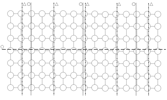
Figure 1: Controllability (observability) partition for a $7\times 15$ grid graph.

Clearly, all the nodes that are not crossed by any line are controllable (observable). Also, a subset of nodes from which the graph is controllable (observable) can be easily constructed by suitably combining the different symbols. Equivalently, given a set of control (observation) nodes, testing the associated symbols easily gives the controllability (observability) property from the given set of nodes. For example, from the pair of nodes $i_{1}=[1,2]$ and $i_{2}=[4,1]$ the grid is not controllable (observable). Indeed, the partitions are $O_{1}=[3,7]$ and $O_{2}=[3,7]\cup[5,7]$ whose intersection is $[3,7]$. The uncontrollable (unobservable) eigenvalues are, according to Theorem III.6, $1+(2-2\cos\frac{\pi}{7})$, $1+(2-2\cos\frac{3\pi}{7})$ and $1+(2-2\cos\frac{5\pi}{7})$. Following the same logic the grid is controllable (observable) form the set $[1,2]$ and $[1,3]$, but it is not controllable (observable) from $[1,2]$, $[1,8]$ and $[4,1]$ (and from any subset of them). We let the reader play with it and have fun.

IV Eigenstructure of general grid graphs

In order to characterize the controllability and observability of general grid graphs we need to exploit their eigenstructure. Indeed, the main difference with respect to the simple case analysis relies in the structure of the uncontrollable (unobservable) eigenvectors. While for simple grids they can be always written as the Kronecker product of two eigenvectors of the path (because the eigenvalues are all simple), this property does not hold for the eigenvectors of non-simple grids. Thus, the controllability (observability) analysis can not be performed by simply looking at how the zeros of the path eigenvectors propagate into the grid. Indeed, this analysis provides only necessary conditions for controllability (observability).

This section will be organized as follows. First, we characterize symmetries in the structure of the grid eigenvectors. This analysis allows us to recognize the components of the eigenvectors that have to be equal. Second, we provide conditions to show what are all and only the components that are zero when a given component is forced to zero. Thus, with this results in hand, we are able to provide necessary and sufficient conditions for controllability (observability).

We begin by characterizing symmetries of the path eigenvectors and then, using these results, we characterize symmetries of the grid eigenvectors by suitable grid partitions. For the sake of clarity we provide the analysis and results for two dimensional grids ($d=2$). The results for higher dimensions are based on the same arguments and will be discussed in a remark.

IV-A Symmetries of the path Laplacian eigenvectors

We provide results on the structure and symmetries of the Laplacian eigenvectors of a path graph. The next lemma characterizes the symmetry of the path Laplacian eigenvectors.

Lemma IV.1 (Symmetries of the path Laplacian eigenvectors)

Any eigenvector $v$ of the Laplacian of a path graph satisfies either $v=\Pi v$ or $v=-\Pi v$, with $\Pi$ the usual permutation matrix.

Proof:

Let $L\in{\mathbb{R}}^{n\times n}$ be the Laplacian of the path. Straightforward calculations show that $L$ satisfies $L=\Pi L\Pi$. Now, let $v$ be a Laplacian eigenvector, then $\Pi L\Pi v=\lambda v$. Multiplying both sides by $\Pi$ (and remembering that $\Pi^{2}=I$), we get $L\Pi v=\lambda\Pi v$, so that $\Pi v$ is also an eigenvector of $L$ associated to the eigenvalue $\lambda$. Since any eigenvalue of $L$ has multiplicity one, it must hold $v=\alpha\Pi v$, for some nonzero $\alpha\in{\mathbb{R}}$. Using the fact that the linear map $\Pi$ is an isometry (i.e. it preserves the norm), $||\Pi v||=||v||$, it follows straight that either $\alpha=1$ or $\alpha=-1$, which concludes the proof. ∎

In the rest of the paper we will denote $S^{+}$ (respectively $S^{-}$) the set of vectors satisfying $v=\Pi v$ (respectively $v=-\Pi v$). An important property of $S^{+}$ and $S^{-}$ is that one is the orthogonal complement of the other, i.e. $(S^{+})^{\perp}=S^{-}$.

The next lemma relates the eigenstructure of a given path $P$ to the eigenstructure of any path with length multiple of the length of $P$.

Lemma IV.2 (Laplacian eigenstructure of $P_{n}$ and $P_{kn}$)

Let $\lambda_{1},\ldots,\lambda_{n}$ be the eigenvalues of the Laplacian $L_{n}$ of a path $P_{n}$ of length $n$ and $v_{1},\ldots,v_{n}$ the corresponding eigenvectors. Then any path $P_{kn}$ of length $kn$, for some $k\in{\mathbb{N}}$, with Laplacian matrix $L_{kn}$ satisfies:

1. $\lambda_{1},\ldots,\lambda_{n}$ are eigenvalues of $L_{kn}$;

2. each eigenvector $w_{i}\in{\mathbb{R}}^{kn}$ of $L_{kn}$ associated to $\lambda_{i}$, $i\in\{1,\dots,n\}$, has the form

   $$w_{i}=\begin{bmatrix}v_{i}^{T}&(\Pi v_{i})^{T}&v_{i}^{T}&\ldots\end{bmatrix}^{T}.$$

Proof:

For the sake of clarity we prove the statement for $k=3$, but the proof for the general case is easily generalizable. The Laplacian $L_{kn}$ can be written in terms of $L_{n}$, whose structure is given in Appendix, as

$$L_{kn}=\begin{bmatrix}L_{n}+e_{n}e_{n}^{T}&-e_{n}e_{1}^{T}&0\\[5.16663pt] -e_{1}e_{n}^{T}&L_{n}+e_{1}e_{1}^{T}+e_{n}e_{n}^{T}&-e_{n}e_{1}^{T}\\[5.16663pt] 0&-e_{1}e_{n}^{T}&L_{n}+e_{1}e_{1}^{T}\end{bmatrix}.$$

Now, let us write the eigenvector $w_{i}$ associated to $\lambda_{i}$ as $w_{i}=\begin{bmatrix}v_{a}^{T}&v_{b}^{T}&v_{c}^{T}\end{bmatrix}^{T}$, with $v_{a}$, $v_{b}$ and $v_{c}$ in ${\mathbb{R}}^{n}$. Thus $w_{i}$ satisfies

$$L_{kn}w_{i}=\begin{bmatrix}L_{n}v_{a}+e_{n}\big{(}(v_{a})_{n}-(v_{b})_{1}\big{)}\\[5.16663pt] L_{n}v_{b}+e_{1}\big{(}(v_{b})_{1}-(v_{a})_{n}\big{)}+e_{n}\big{(}(v_{b})_{n}-(v_{c})_{1}\big{)}\\[5.16663pt] L_{n}v_{c}+e_{1}\big{(}(v_{c})_{1}-(v_{b})_{n}\big{)}\end{bmatrix}$$

Now let us take $v_{a}=v_{i}$, $v_{b}=\Pi v_{i}$ and $v_{c}=v_{i}$, then

$$\begin{split}L_{kn}w_{i}&=\lambda_{i}w_{i}+\begin{bmatrix}e_{n}\big{(}(v_{i})_{n}-(\Pi v_{i})_{1}\big{)}\\[5.16663pt] e_{1}\big{(}(\Pi v_{i})_{1}-(v_{i})_{n}\big{)}+e_{n}\big{(}(\Pi v_{i})_{n}-(v_{i})_{1}\big{)}\\[5.16663pt] e_{1}\big{(}(v_{i})_{1}-(\Pi v_{i})_{n}\big{)}\end{bmatrix}=\lambda_{i}w_{i}.\end{split}$$

Last equality follows by the fact that $(\Pi v_{i})_{1}=(v_{i})_{n}$ and $(\Pi v_{i})_{n}=(v_{i})_{1}$ (in general $(\Pi v_{i})_{\ell}=(v_{i})_{n-\ell+1}$ for any $\ell\in\{1,\dots,n\}$). ∎

Exploiting the result in the above lemma by using the result in Lemma IV.1, it follows easily that $w_{i}=\begin{bmatrix}v_{i}^{T}&v_{i}^{T}&v_{i}^{T}&\ldots\end{bmatrix}^{T}$ for $v_{i}=\Pi v_{i}$ (and thus $w_{i}=\Pi w_{i}$) and $w_{i}=~{}\begin{bmatrix}v_{i}^{T}&-v_{i}^{T}&v_{i}^{T}&\ldots\end{bmatrix}^{T}$ for $v_{i}=-\Pi v_{i}$ (and thus $w_{i}=-\Pi w_{i}$).

IV-B Symmetries of the grid eigenvectors

Next, we provide tools to recognize symmetries in the grid eigenvectors, based on the graph structure, which will play a key role in the controllability (observability) analysis.

Without loss of generality, let $\lambda=\lambda_{1,1}+\lambda_{1,2}=\ldots=\lambda_{\mu,1}+\lambda_{\mu,2}$ be an eigenvalue of geometric multiplicity $\mu\in{\mathbb{N}}$, with $\lambda_{1,1},\ldots,\lambda_{\mu,1}$ (respectively $\lambda_{1,2},\ldots,\lambda_{\mu,2}$) eigenvalues of $P_{1}$ (respectively $P_{2}$) and corresponding eigenvectors $v_{1},\ldots v_{\mu}$ (respectively $w_{1},\ldots,w_{\mu}$). The corresponding eigenspace $V_{\lambda}$ is given by

$$V_{\lambda}=\{v\in{\mathbb{R}}^{n_{1}\cdot n_{2}}|v=\sum_{i=1}^{\mu}\alpha_{i}(v_{i}\otimes w_{i}),\alpha_{i}\in{\mathbb{R}}\}.$$ (6)

As mentioned at the beginning of this section, it is worth noting that the eigenvectors in $V_{\lambda}$ do not necessarily have the structure of a Kronecker product of two eigenvectors (the set of vectors expressed as Kronecker product is not closed under linear combination). For this reason, in order identify all and only the zero components of these eigenvectors, we need to characterize their structure.

Remark IV.3

For each node $[\nu,\ell]$ such that the paths $P_{1}$ and $P_{2}$ are controllable (observable) from $\nu$ and $\ell$ respectively, all the basis eigenvectors of $V_{\lambda}$ have nonzero $[\nu,\ell]$ component. $\square$

Before stating the main results of this section, we need to introduce some useful notation. Given a path $P_{n}$ of length $n\in{\mathbb{N}}$, for $\{i,j\}\subset\{1,\dots,n\}$, $i<j$, we denote $P_{i:j}$ the sub-path of $P_{n}$ with node set $\{i,\dots,j\}$ (e.g., $P_{2:4}$ is the sub-path with node set {2,3,4}). Let $G=P_{l\cdot n_{1}}\Box P_{m\cdot n_{2}}$ with $P_{l\cdot n_{1}}$ of dimension $l\cdot n_{1}$ and $P_{m\cdot n_{2}}$ of dimension $m\cdot n_{2}$. We call $G_{ij}=P_{((i-1)n_{1}+1):(in_{1})}\Box P_{((j-1)n_{2}+1):(jn_{2})}$, for $i\in\{1,\dots,l\}$ and $j\in\{1,\dots,m\}$, an $n_{1}\times n_{2}$ sub-grid or a brick of $G$, see Figure 2.

Figure 2: Partition of a grid into bricks

Let $v\in{\mathbb{R}}^{l\cdot n_{1}\cdot m\cdot n_{2}}$ be a vector of $G$, we call the sub-vector of $v$ associated to $G_{ij}$ the vector $v_{ij}\in{\mathbb{R}}^{n_{1}\cdot n_{2}}$ with components $(v_{ij})_{[\nu,\,\ell]}$, $\nu\in\{1,\dots,n_{1}\}$ and $\ell\in\{1,\dots,n_{2}\}$, given by $(v_{ij})_{[\nu,\,\ell]}=(v)_{[(i\text{-}1)n_{1}\text{+}\nu,\,(j\text{-}1)n_{2}\text{+}\ell]}$. Informally, the sub-vector $v_{ij}$ of $v$ is constructed by selecting the components of $v$ that fall into the brick $G_{ij}$.

Next, given a grid $G=P_{n_{1}}\Box P_{n_{2}}$, with $P_{n_{1}}$ and $P_{n_{2}}$ paths of length $n_{1}$ and $n_{2}$ respectively, we introduce two useful operators that flip the components of a vector $v$ associated to a grid $G$. Formally, consider the matrices

$$(\Pi_{n_{1}}\otimes I_{n_{2}})=\begin{bmatrix}0_{n_{2}\times n_{2}}&\ldots&I_{n_{2}}\\[5.16663pt] &\iddots&\\[5.16663pt] I_{n_{2}}&\ldots&0_{n_{2}\times n_{2}}\\[5.16663pt] \end{bmatrix}\;\text{and}\;\;(I_{n_{1}}\otimes\Pi_{n_{2}})=\begin{bmatrix}\Pi_{n_{2}}&\ldots&0_{n_{2}\times n_{2}}\\[5.16663pt] &\ddots&\\[5.16663pt] 0_{n_{2}\times n_{2}}&\ldots&\Pi_{n_{2}}\\[5.16663pt] \end{bmatrix}.$$

These operators flip respectively the first and the second sets of components. Formally, given a vector $v\in{\mathbb{R}}^{n_{1}\cdot n_{2}}$ associated to the grid $G$, with components $(v)_{[\nu,\,\ell]}$, $\nu\in\{1,\dots,n_{1}\}$ and $\ell\in\{1,\dots,n_{2}\}$, let $v_{1}=(\Pi_{n_{1}}\otimes I_{n_{2}})v$ and $v_{2}=(I_{n_{1}}\otimes\Pi_{n_{2}})v$. The vectors $v_{1}$ and $v_{2}$ are related to $v$ by

$$(v_{1})_{[\nu,\,\ell]}=(v)_{[n_{1}-\nu+1,\,\ell]},\;\;\text{and}\;\;(v_{2})_{[\nu,\,\ell]}=(v)_{[\nu,\,n_{2}-\ell+1]},$$

for $\nu\in\{1,\dots,n_{1}\}$ and $\ell\in\{1,\dots,n_{2}\}$. Finally, the composition of the two operators satisfies $(\Pi_{n_{1}}\otimes I_{n_{2}})(I_{n_{1}}\otimes\Pi_{n_{2}})=(\Pi_{n_{1}}\otimes\Pi_{n_{2}})$. Thus, when applied to a vector $v$, the composed operator flips both sets of components. That is, denoting $v_{3}=(\Pi_{n_{1}}\otimes\Pi_{n_{2}})v$, we have

$$(v_{3})_{[\nu,\,\ell]}=(v)_{[n_{1}-\nu+1,\,n_{2}-\ell+1]},$$

for $\nu\in\{1,\dots,n_{1}\}$ and $\ell\in\{1,\dots,n_{2}\}$.

Lemma IV.4

Let $G_{0}=P_{n_{1}}\Box P_{n_{2}}$ with $P_{n_{1}}$ and $P_{n_{2}}$ paths of length respectively $n_{1}$ and $n_{2}$. Any eigenvalue $\lambda$ of the Laplacian $L_{0}$ of $G_{0}$ is an eigenvalue of the Laplacian $L$ of $G=P_{l\cdot n_{1}}\Box P_{m\cdot n_{2}}$ for any $l\in{\mathbb{N}}$ and $m\in{\mathbb{N}}$.

Proof:

From Lemma III.1, each eigenvalue $\lambda_{0}$ of $G_{0}$ (respectively $\lambda$ of $G$) can be written as $\lambda_{0}=\lambda_{01}+\lambda_{02}$ ($\lambda=\lambda_{1}+\lambda_{2}$) where $\lambda_{01}$ ($\lambda_{1}$) is an eigenvalue of $P_{n_{1}}$ ($P_{l\cdot n_{1}}$) and $\lambda_{02}$ ($\lambda_{2}$) of $P_{n_{2}}$ ($P_{m\cdot n_{2}}$). From Lemma IV.2 all the eigenvalues of $P_{n_{1}}$ ($P_{n_{2}}$) are eigenvalues of $P_{l\cdot n_{1}}$ ($P_{m\cdot n_{2}}$) so that the proof follows. ∎

We are now ready to characterize the eigenvector symmetries by suitable brick partitions.

Theorem IV.5 (Grid partition and eigenvector symmetries)

Let $G_{0}=P_{n_{1}}\Box P_{n_{2}}$ be a grid of dimension $n_{1}\times n_{2}$ with $P_{n_{1}}$ and $P_{n_{2}}$ paths of dimension respectively $n_{1}$ and $n_{2}$. Take any grid $G=P_{l\cdot n_{1}}\Box P_{m\cdot n_{2}}$ of dimension $ln_{1}\times mn_{2}$ and let $G_{ij}$, $i\in\{1,\dots,l\}$ and $j\in\{1,\dots,m\}$, be a partition into bricks of dimension $n_{1}\times n_{2}$.

Then for each eigenvalue (possibly non-simple) $\lambda$ of $L_{0}$:

1. $\lambda$ is an eigenvalue of $L$, and

2. any eigenvector $v$ of $L$ associated to $\lambda$ can be decomposed into sub-vectors $v_{ij}$ relative to the bricks $G_{ij}$ with

   $$v_{ij}=(\Pi_{n_{1}}\otimes I_{n_{2}})^{(i-1)}(I_{n_{1}}\otimes\Pi_{n_{2}})^{(j-1)}v_{0}$$

   for $i\in\{1,\dots,n_{1}\}$ and $j\in\{1,\dots,n_{2}\}$, where $v_{0}$ is an eigenvector of $L_{0}$ associated to $\lambda$.

Proof:

Statement (i) follows straight by Lemma IV.4. To prove statement (ii), first, let us recall that the matrices $(\Pi_{n_{1}}\otimes I_{n_{2}})$ and $(I_{n_{1}}\otimes\Pi_{n_{2}})$ applied to the vectors $v_{0}$ respectively flip the first and second components. Also, $(\Pi_{n_{1}}\otimes I_{n_{2}})^{(i-1)}w=w$ for $i$ odd (respectively $(I_{n_{1}}\otimes\Pi_{n_{2}})^{(j-1)}w=w$ for $j$ odd). Thus, we can just prove the result for $(i,j)=(0,1)$ and $(i,j)=(1,0)$.

Let $\mu$ be the geometric multiplicity of the eigenvalue $\lambda$ for the Laplacian $L$. Then, by Lemma III.1, a basis of the associated eigenspace $V_{\lambda}$ is given by $\mu$ vectors obtained as the Kronecker product of eigenvectors of the constitutive path graphs. That is,

$$V_{\lambda}=\{v\in{\mathbb{R}}^{n_{1}\cdot n_{2}}|v=\sum_{i=1}^{\mu}\alpha_{i}(v_{i}\otimes w_{i}),\alpha_{i}\in{\mathbb{R}}\},$$

where $v_{i}$ and $w_{i}$, $i\in\{1,\dots,\mu\}$ are eigenvectors of respectively $P_{n_{1}}$ and $P_{n_{2}}$ associated to eigenvalues $\lambda_{i,1}$ and $\lambda_{i,2}$ such that $\lambda_{i,1}+\lambda_{i,2}=\lambda$. Exploiting the Kronecker product and using the result in Lemma IV.2, we have

$$\begin{split}v=\sum_{i=1}^{\mu}\alpha_{i}\left[(v_{i})_{1}\begin{bmatrix}w_{i}\\ \Pi w_{i}\\ w_{i}\\ \vdots\end{bmatrix}^{T}\;\;\ldots\;\;(v_{i})_{n_{1}}\begin{bmatrix}w_{i}\\ \Pi w_{i}\\ w_{i}\\ \vdots\end{bmatrix}^{T}\;\;\vline\;\;\right.\left.(\Pi v_{i})_{1}\begin{bmatrix}w_{i}\\ \Pi w_{i}\\ w_{i}\\ \vdots\end{bmatrix}^{T}\;\;\ldots\;(\Pi v_{i})_{n_{1}}\begin{bmatrix}w_{i}\\ \Pi w_{i}\\ w_{i}\\ \vdots\end{bmatrix}^{T}\;\vline\ldots\right]^{T}.\end{split}$$

Clearly, the brick $G_{11}$ coincides with the grid $G_{0}$. Thus, we can compare the bricks $G_{ij}$ with the brick $G_{11}$. The sub-eigenvector corresponding to the “first row” of the brick $G_{11}$ is given by

$$(v_{11})_{[1,\,1:n_{1}]}:=\begin{bmatrix}(v_{11})_{[1,1]}\\ \vdots\\ (v_{11})_{[1,n_{1}]}\\ \end{bmatrix}=\alpha_{i}(v_{i})_{1}w_{i}$$

Using the definition of brick components, the sub-eigenvectors corresponding to the “first row” of the grid $G_{12}$ is

$$\begin{split}(v_{12})_{[1,\,1:n_{1}]}:=\begin{bmatrix}(v_{12})_{[1,1]}\\ \vdots\\ (v_{12})_{[1,n_{1}]}\\ \end{bmatrix}=\alpha_{i}(v_{i})_{1}\Pi w_{i}=\alpha_{i}(v_{i})_{1}\begin{bmatrix}(w_{i})_{n}\\ \vdots\\ (w_{i})_{1}\\ \end{bmatrix}=\begin{bmatrix}(v_{11})_{[1,n_{1}]}\\ \vdots\\ (v_{11})_{[1,1]}\\ \end{bmatrix}.\end{split}$$

The proof for the other components follows exactly the same arguments. ∎

The above theorem has a nice and intuitive graphical interpretation, as shown in Figure 3.

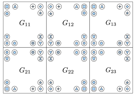
Figure 3: Graphical interpretation of Theorem IV.5

Given a grid $G$ and an eigenvector $v$ associated to an eigenvalue $\lambda$, we can associate a symbol to each node depending on the value of the eigenvector component. Then, we partition the grid $G$ into bricks of dimension $n_{1}\times n_{2}$. Given the symbols in the brick $G_{11}$, the symbols in a brick $G_{i,j}$, for $i\in\{1,\dots,l\}$ and $j\in\{2,\dots,m\}$, are obtained by a reflection of the brick $G_{i,j-1}$ with respect to the horizontal axis, while the symbols in a brick $G_{i,j}$, for $i\in\{2,\dots,l\}$ and $j\in\{1,\dots,m\}$, are obtained by a reflection of the brick $G_{i-1,j}$ with respect of the vertical axis.

Next, we analyze the eigenvector components of a brick whose dimensions are prime or, equivalently, the components of eigenvectors associated to eigenvalues that are not eigenvalues of smaller bricks. Recalling that any path eigenvector $v$ satisfies either $v=\Pi v$ ($v\in S^{+}$) or $v=-\Pi v$ ($v\in S^{-}$), we show how: (i) each basis eigenvector has a symmetry induced by the symmetry of the path eigenvectors, and (ii) the structure of a general grid eigenvector is influenced by the symmetry of the basis eigenvectors.

Proposition IV.6

Let $G_{0}=P_{n_{1}}\Box P_{n_{2}}$ be a grid of dimension $n_{1}\times n_{2}$. For any eigenvalue $\lambda$, let $V_{\lambda}$ be the associated eigenspace, with structure as in equation (6). Then, each basis eigenvector generating $V_{\lambda}$, $(v_{i}\otimes w_{i})$, satisfies one of the four relations:

$$\begin{split}(v_{i}\otimes w_{i})&=\phantom{-}(\Pi\otimes I)(v_{i}\otimes w_{i})=\phantom{-}(I\otimes\Pi)(v_{i}\otimes w_{i})\\ (v_{i}\otimes w_{i})&=\phantom{-}(\Pi\otimes I)(v_{i}\otimes w_{i})=-(I\otimes\Pi)(v_{i}\otimes w_{i})\\ (v_{i}\otimes w_{i})&=-(\Pi\otimes I)(v_{i}\otimes w_{i})=\phantom{-}(I\otimes\Pi)(v_{i}\otimes w_{i})\\ (v_{i}\otimes w_{i})&=-(\Pi\otimes I)(v_{i}\otimes w_{i})=-(I\otimes\Pi)(v_{i}\otimes w_{i}).\\ \end{split}$$

Proof:

Using the result in Lemma IV.1, $v_{i}$ and $w_{i}$ belong either to $S^{+}$ or $S^{-}$, that is, e.g., either $v_{i}=\Pi v_{i}$ or $v_{i}=-\Pi v_{i}$. Suppose that, for example, $v_{i}\in S^{+}$ and $w_{i}\in S^{-}$. Under this assumption $(v_{i}\otimes w_{i})=(\Pi v_{i}\otimes w_{i})=(\Pi v_{i}\otimes Iw_{i})$ and, using the distributive property of the Kronecker product $(v_{i}\otimes w_{i})=(\Pi\otimes I)(v_{i}\otimes w_{i})$. Also, $(v_{i}\otimes w_{i})=(v_{i}\otimes-\Pi w_{i})=(Iv_{i}\otimes-\Pi w_{i})=-(I\otimes\Pi)(v_{i}\otimes w_{i})$. This gives the second of the four relations. The other three cases follow by the other three possible combinations of the symmetries of $v_{i}$ and $w_{i}$, thus concluding the proof. ∎

In the following we denote the set of vectors satisfying each one of the four relations in the proposition respectively as $S^{++}$, $S^{+-}$, $S^{-+}$ and $S^{--}$. A graphical representation of the four sets is given in Figure 4.

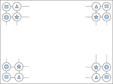
(a) symmetry class $S^{++}$

(b) symmetry class $S^{+-}$

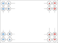
(c) symmetry class $S^{-+}$

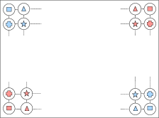
(d) symmetry class $S^{--}$

Figure 4: Graphical interpretation of Proposition IV.6

We associate a symbol to each node depending on the value of the eigenvector component. Also, we denote with the same symbol but different colors nodes that have components of opposite sign. The result in Proposition IV.6 can be easily explained by using this graphical interpretation. Namely, each of the four cases in the proposition correspond to a scheme in Figure 4.

The next remark gives an insight on the eigenvector components of the “central” nodes of a grid with odd dimensions.

Remark IV.7 (Symmetries for grids with prime dimensions)

If the grid has odd dimensions, $n_{1}$ and $n_{2}$, the above symmetries have interesting implications for the nodes with components respectively $[\frac{n_{1}+1}{2},\ell]$, $\ell\in\{1,\dots,n_{1}\}$, and $[\nu,\frac{n_{2}+1}{2}]$, $\nu\in\{1,\dots,n_{2}\}$. Indeed, the first set of components is zero for $S^{-+}$ and $S^{--}$, while the second one is zero for $S^{+-}$ and $S^{--}$. $\square$

This proposition has an important impact on the symmetries of general eigenvectors belonging to the same eigenspace (and in particular for each brick of a general grid). Clearly, if an eigenvalue is simple, then any associated eigenvector has the structure of a Kronecker product and thus one of the four symmetries. For a non-simple eigenvalue, any eigenvector of $V_{\lambda}$ can be written as a linear combination of the basis vectors, and thus, using the proposition, by the sum of at most four vectors each one having one of the four symmetries. Thus, in order to identify the symmetries of a general vector, we need to “suitably combine” nodes with the same symbol and color in different classes. Three cases are possible: (i) if basis vectors of at least three different classes are present, by inspection in Figure 4, no symmetries are present, (ii) if all basis vectors belong to the same class, then also the linear combination does, and (iii) if the basis vectors belong to two of the four classes, a general eigenvector $v$ (obtained as their linear combination) satisfies the following symmetries:

• $(v)_{[\nu,\ell]}=\pm(v)_{[n_{1}-\nu+1,\ell]}$ if the two classes share the first symbol (e.g., $S^{++}$ and $S^{+-}$);

• $(v)_{[\nu,\ell]}=\pm(v)_{[\nu,n_{2}-\ell+1]}$ if the two classes share the second symbol (e.g., $S^{++}$ and $S^{-+}$);

• $(v)_{[\nu,\ell]}=\pm(v)_{[n_{1}-\nu+1,n_{2}-\ell+1]}$ if the two classes share no symbol (e.g., $S^{++}$ and $S^{--}$).

A graphical representation of the above three symmetries is depicted in Figure 5. We associate the same symbol to nodes having the same absolute value of the eigenvector component. It is worth noting that we are interested in the absolute values because we want to classify all the components that can be zeroed simultaneously.

(a) first symbol in common

(b) second symbol in common

(c) no symbol in common

Figure 5: Symmetries of eigenvectors obtained as the sum of basis vectors of two different classes.

V Controllability and observability analysis of general grid graphs

In this section we provide necessary and sufficient conditions to characterize all and only the nodes from which the network system is controllable (observable). First, we need a well known result in linear systems theory, see, e.g., [33]. We state it for the controllability property.

Lemma V.1

If a state matrix $A\in{\mathbb{R}}^{n\times n}$, $n\in{\mathbb{N}}$, has an eigenvalue with geometric multiplicity $\mu\in{\mathbb{N}}$, then for any $B\in{\mathbb{R}}^{n\times m}$ with $m<\mu$ the pair $(A,B)$ is uncontrollable. $\square$

The previous lemma applied to the grid Laplacian says that, in case the grid is non simple with maximum eigenvalue multiplicity $\mu$, then the grid is not controllable (observable) from a set of control (observation) nodes of cardinality less than $\mu$.

Using Lemma II.1, it follows straight that we can study the controllability (observability) properties of the grid separately for each eigenvalue. Namely, to guarantee controllability (observability), we need to show that for each eigenvalue of the grid Laplacian $L$, there does not exist any eigenvector satisfying the condition in (2), i.e. having zero in some components.

If $\lambda$ is simple, the corresponding eigenspace $V_{\lambda}$ in (6) is given by $V_{\lambda}=\{v\in{\mathbb{R}}^{n_{1}\cdot n_{2}}|v=\alpha_{1}(v_{1}\otimes w_{1}),\alpha_{1}\in{\mathbb{R}}\}.$ Thus, finding the zeros of any eigenvector in $V_{\lambda}$ is equivalent to finding the zeros of the eigenvectors $v_{1}$ and $w_{1}$ and propagate them according to the Kronecker product structure. Clearly, with this observation in hand, the analysis of any simple eigenvalue can be performed by using the tools provided in Section III.

For eigenvalues with multiplicity greater than one, next two considerations are important. First, not all the eigenvectors of $\lambda$ have the structure of a Kronecker product. Second, consistently with Lemma V.1, it is always possible to find an eigenvector $v\in V_{\lambda}$ with an arbitrary component equal to zero, for a suitable choice of the coefficients $\alpha_{i}$ in (6). Thus, the controllability (observability) analysis does not depend only on the zero components of the path eigenvectors, but also on the symmetries in the grid eigenvector components. That is, for the eigenvalue under investigation, we want to answer to the following question. If we find an eigenvector with zero in an arbitrary component $\ell$, what are all and only the other components that are zero in the chosen eigenvector? We provide the analysis for non-simple eigenvalues of multiplicity two and discuss the generalization in a remark.

On the basis of the eigenvector symmetries identified in Theorem IV.5, we can study the controllability (observability) of a brick.

Next lemma provides useful properties of the eigenvector components in a brick.

Lemma V.2 (Polynomial structure of the eigenvector components)

Let $G_{0}=P_{n_{1}}\Box P_{n_{2}}$ be a grid of dimension $n_{1}\times n_{2}$. Then, any Laplacian eigenvector $u=v\otimes w$ of the grid, with $v$ and $w$ respectively eigenvectors of $P_{n_{1}}$ and $P_{n_{2}}$ associated to eigenvalues $\lambda_{v}$ and $\lambda_{w}$, has components $(u)_{[\nu,\ell]}$, $\nu\in\{1,\dots,n_{1}\}$ and $\ell\in\{1,\dots,n_{2}\}$ satisfying

1. $(u)_{[\nu,\ell]}=p_{\nu}(\lambda_{v})\cdot p_{\ell}(\lambda_{w})\cdot(v)_{1}\cdot(w)_{1}$, where $p_{r}(s)$ is the polynomial of degree $(r-1)$ defined as $p_{2}(s)=1-s$ for $r=2$ and, denoting $p_{1}(s)=1$, by the recursion

   $$p_{r}(s)=(2-s)p_{r-1}(s)-p_{r-2}(s)$$ (7)

   for $r\geq 3$;

2. if $n_{1}$ and $n_{2}$ prime, then $p_{\nu}(\lambda_{v})\neq 0$ and $p_{\ell}(\lambda_{w})\neq 0$ for any $\nu\in\{1,\dots,\frac{n_{1}-1}{2}\}$ and $\ell\in\{1,\dots,\frac{n_{2}-1}{2}\}$.

Proof:

First, notice that $(u)_{[\nu,\ell]}=(v)_{\nu}\cdot(w)_{\ell}$. To prove statement (i), we need to prove that for a path of length $n_{1}$, any eigenvector $v$ satisfies $(v)_{\nu}=p_{\nu}(\lambda_{v})(v)_{1}$ for $\nu\in\{1,\dots,n_{1}\}$. We prove the statement by induction. We exploit the eigenvector relation $L_{n_{1}}v=\lambda_{v}v$ by using the structure of the path Laplacian given in Appendix. From the first row, it follows that $(v)_{1}-(v)_{2}=\lambda_{v}(v)_{1}$, so that $(v)_{2}=(1-\lambda_{v})(v)_{1}$. Then, from the $r$th row of the relation, we have $-(v)_{r-1}+2(v)_{r}-(v)_{r+1}=\lambda_{v}(v)_{r}$ and thus $(v)_{r+1}=(2-\lambda_{v})(v)_{r}-(v)_{r-1}$. Plugging in the inductive assumption $(v)_{r}=p_{r}(\lambda_{v})(v)_{1}$ and $(v)_{r-1}=p_{r-1}(\lambda_{v})(v)_{1}$, we have $(v)_{r+1}=p_{r+1}(\lambda_{v})(v)_{1}$ with $p_{r+1}(\lambda_{v})=(2-\lambda_{v})p_{r}(\lambda_{v})-p_{r-1}(\lambda_{v})$ which concludes the first part of the proof.

Statement (ii) can be proven by showing that, for a path graph of length $n_{1}$ with $n_{1}$ prime, any eigenvector $v$ has non zero components $(v)_{1}$, $\ldots$, $(v)_{\frac{n_{1}-1}{2}}$. This result is proven in [7], thus concluding the proof. ∎

Next theorem gives necessary and sufficient conditions for two eigenvector components to be both zero in a brick.

Theorem V.3 (Simultaneous zeroing of eigenvector components)

Let $G_{0}=P_{n_{1}}\Box P_{n_{2}}$ be a grid of dimension $n_{1}\times n_{2}$. Let $\lambda=\lambda_{1,1}+\lambda_{1,2}=\lambda_{2,1}+\lambda_{2,2}$ be an eigenvalue of multiplicity two, with $\lambda_{1,1}$ and $\lambda_{2,1}$ ($\lambda_{1,2}$ and $\lambda_{2,2}$) eigenvalues of $P_{n_{1}}$ ($P_{n_{2}}$). Let $V_{\lambda}$ be the associated eigenspace. Then there exists an eigenvector $v\in V_{\lambda}$ with zero components $[\nu_{1},\ell_{1}]$ and $[\nu_{2},\ell_{2}]$, $\nu_{1},\nu_{2}\in\{1,\dots,n_{1}\}$ and $\ell_{1},\ell_{2}\in\{1,\dots,n_{2}\}$, if and only if

$$p_{\nu_{1}}(\lambda_{1,1})\cdot p_{\ell_{1}}(\lambda_{1,2})\cdot p_{\nu_{2}}(\lambda_{2,1})\cdot p_{\ell_{2}}(\lambda_{2,2})=\;p_{\nu_{1}}(\lambda_{2,1})\cdot p_{\ell_{1}}(\lambda_{2,2})\cdot p_{\nu_{2}}(\lambda_{1,1})\cdot\;p_{\ell_{2}}(\lambda_{1,2}),$$ (8)

where $p_{r}(s)$ is the polynomial of degree $r-1$ defined by the recursion in equation (7).

Proof:

To prove the statement, we look for an eigenvector $v=\alpha_{1}(v_{1}\otimes w_{1})+\alpha_{2}(v_{2}\otimes w_{2})$ with $\alpha_{1}$ and $\alpha_{2}$ such that $(v)_{[\nu_{1},\ell_{1}]}=0$ and $(v)_{[\nu_{2},\ell_{2}]}=0$. The condition $(v)_{[\nu_{1},\ell_{1}]}=0$ is equivalent to $\alpha_{1}(v_{1})_{\nu_{1}}(w_{1})_{\ell_{1}}+\alpha_{2}(v_{2})_{\nu_{1}}(w_{2})_{\ell_{1}}=0$. From Lemma V.2 (i) we have $\alpha_{1}\,p_{\nu_{1}}(\lambda_{1,1})\cdot(v_{1})_{1}\cdot p_{\ell_{1}}(\lambda_{2,1})\cdot(w_{1})_{1}+\alpha_{2}\,p_{\nu_{1}}(\lambda_{1,2})\cdot(v_{2})_{1}\cdot p_{\ell_{1}}(\lambda_{2,2})\cdot(w_{2})_{1}=0$. Using the same calculations for the condition $(v)_{[\nu_{2},\ell_{2}]}=0$, we can write the matrix equation

$$\begin{bmatrix}p_{\nu_{1}}(\lambda_{1,1})p_{\ell_{1}}(\lambda_{1,2})(v_{1})_{1}(w_{1})_{1}\;&\;p_{\nu_{1}}(\lambda_{2,1})p_{\ell_{1}}(\lambda_{2,2})(v_{2})_{1}(w_{2})_{1}\\[5.16663pt] p_{\nu_{2}}(\lambda_{1,1})p_{\ell_{2}}(\lambda_{1,2})(v_{1})_{1}(w_{1})_{1}\;&\;p_{\nu_{2}}(\lambda_{2,1})p_{\ell_{2}}(\lambda_{2,2})(v_{2})_{1}(w_{2})_{1}\end{bmatrix}\begin{bmatrix}\alpha_{1}\\ \alpha_{2}\end{bmatrix}=0.$$ (9)

Since $v$ is an eigenvector, $\alpha_{1}$ and $\alpha_{2}$ can not be zero simultaneously. Thus, the above equation is satisfied if and only if the matrix is singular. Imposing the condition that the determinant be zero gives equation (8). ∎

Remark V.4 (Extensions to higher grid dimension and eigenvalue multiplicity)

If the grid is of dimension $d>2$ the above theorem extends in a straightforward manner. Indeed, the result in Lemma V.2 (i) can be easily generalized as $(u)_{[i_{1},\ldots,i_{d}]}=p_{i_{1}}(\lambda_{i_{1}})\cdot\ldots\cdot p_{i_{d}}(\lambda_{i_{d}})\cdot(v_{1})_{1}\cdot\ldots\cdot(v_{d})_{1}$, with suitable adaptation of the notation, so that the condition in equation (8) follows straight.

If the grid has an eigenvalue of multiplicity $\mu>2$, then the theorem generalizes by considering $\mu$ nodes. The condition in equation (8) follows by setting to zero the determinant of a $\mu\times\mu$ version of the matrix in (9) with elements $(i,j)\in\{1,\dots,\mu\}\times\{1,\dots,\mu\}$ given by $p_{\nu_{i}}(\lambda_{j,1})p_{\ell_{i}}(\lambda_{j,2})(v_{j})_{1}(w_{j})_{1}$. $\square$

Next, we show a graphical interpretation of the controllability (observability) results obtained by combining the results of Theorem III.6, Theorem IV.5, Proposition IV.6 and Theorem V.3. We present it through an example. In Figure 6 we show a two dimensional grid of length $4\times 6$. The analysis for the simple eigenvalues can be performed as explained in Section III. This gives the cross symbol in the set of nodes $[2,i]$ and $[5,i]$, $i\in\{1,\dots,4\}$ in Figure 6 (b). Then, we partition the grid into bricks of dimensions $2\times 2$ and $2\times 3$. The eigenvalue $\lambda_{1}=2$ (respectively $\lambda_{2}=3$) is an eigenvalue of multiplicity two in the brick $2\times 2$ ($2\times 3$). The eigenvectors generating $V_{\lambda_{1}}$ ($V_{\lambda_{2}}$) belong to $S^{+-}$ and $S^{-+}$ ($S^{++}$ and $S^{--}$). This gives the symmetries in Figure 6 (a) according to Proposition IV.6 and the subsequent discussion. Using Theorem V.3 it is easy to verify that all different symbols in Figure 6 (a) correspond, in fact, to distinct component values. Replicating the brick symbols according to Theorem IV.5 we get the structure in Figure 6 (b). Notice that in this particular case we have used the same cross symbol both for the non-simple eigenvalue $\lambda=3$ and for the simple eigenvalues. Finally, it can be easily tested that $\lambda_{1}=2$ and $\lambda_{2}=3$ are the only two non-simple eigenvalues. Given a set of control (observation) nodes, the grid is controllable (observable) if and only if the nodes do not have any symbol in common. If, for example, the control (observation) nodes share the top symbol, then the eigenvalue $\lambda=2$ (of the brick $2\times 2$) is uncontrollable (unobservable). As for the simple case we let the reader play with the rule.

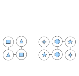
(a) bricks $2$x$2$ & $2$x$3$

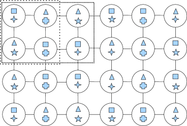
(b) brick partition

Figure 6: Graphical interpretation of the controllability and observability analysis.

To conclude, we provide a discussion on the importance and the effectiveness of the proposed methodologies in studying the controllability and observability (in general the dynamics) of grid graph induced systems. First, we want to stress the fact that the proposed tools give strong insights on the structure and symmetries of the grid eigenvectors and of the controllable (unobservable) subspaces, as shown, e.g., in the above example. Furthermore, the proposed tools represent, clearly, an effective alternative to the standard tests in checking the controllability and observability properties. Notice that, the PBH test in Lemma II.1 (to be performed for each eigenvalue) becomes prohibitive as the dimensions of the grid grow. Similarly, inspecting the rank of the controllability (observability) matrix is an operation that is ill-conditioned as the matrix dimension grows. As opposed to it, our tools involve the following operations. The test on the simple eigenvalues can be done simultaneously by using the tools in Section III and involves only arithmetic operations from number theory. The analysis for non-simple eigenvalues involves the following operations. First, using Theorem IV.5, the grid can be partitioned into bricks of prime dimensions. This operation is based on a straightforward prime number factorization. Second, one has to compute the non simple eigenvalues for each brick. This can be done by using Lemma III.1 and the closed form expression for the path eigenvalues given in Appendix. Third, for each multiple eigenvalue, one has to inspect the symmetries in each brick (again with simple operations on the brick dimensions according to Proposition IV.6) and the possible coincidence of symbols (by means of polynomial evaluations from Theorem V.3). Finally, one should verify if there are multiple eigenvalues of the main grid that are not eigenvalues of smaller bricks. However, so far we have never found such a case in simulations, so that we conjecture that this is unlike or even impossible to happen.

VI Conclusions

In this paper we have characterized the controllability (by duality the observability) of linear time-invariant systems whose dynamics are induced by the Laplacian of a grid (or lattice) graph. We have shown that these systems arise in several fields of application as, in particular, distributed control and estimation, quantum computation and approximate solution of partial differential equations. We have characterized the eigenstructure of the grid Laplacian in terms of suitable graph decompositions and symmetries, and in terms of simple rules from number theory. Based on this analysis, we have shown what are all and only the uncontrollable (unobservable) set of nodes and provided simple routines to choose a set of control (observation) nodes that guarantee controllability (observability).

Appendix A Previous results on the controllability and observability of path and cycle graphs

In this section we briefly recall the results in [6], see also [7], on the controllability (observability) of path graphs. The characterization of the controllability (observability) for grid graphs relies on these results.

Since it is extensively used in the paper, we provide the expression of the path Laplacian, $L_{n}$, and of its distinct eigenvalues $\lambda_{1},\ldots,\lambda_{n}$

$$L_{n}=\begin{bmatrix}\;1&\text{-}1&0&\dots&\;0\\ \text{-}1&\;2&\text{-}1&\dots&\;0\\ \vdots&&\ddots&&\\ \;0&&\text{-}1&\;2&\text{-}1\\ \;0&&\;0&\text{-}1&\;1\\ \end{bmatrix}\quad\text{and}\quad\lambda_{k}=2-2\cos\left((k-1)\frac{\pi}{n}\right),k=1,\ldots,n.$$

The controllability (observability) of the path can be analyzed by using the PBH lemma in the form expressed in Lemma II.1. First, it is known, [35], that a path graph is always controllable (observable) from an external node ($1$ or $n$). Next theorem, which is Theorem 4.4 in [7], completely characterizes the controllability (observability) of a path by means of simple rules from number theory.

Theorem A.1 (Path controllability and observability)

Given a path graph of length $n$, let $n=2^{n_{0}}\prod_{\nu=1}^{k}p_{\nu}$ be a prime number factorization for some $k\in{\mathbb{N}}$ and distinct (odd) prime numbers $p_{1},\ldots,p_{k}$. The following statements hold:

1. the path is not completely controllable (observable) from a node $i\in\{2,\dots,n-1\}$ if and only if

   $$(n-i)\;{\buildrel\rm mod\,p\over{=}}\;(i-1)$$

   for some odd prime $p$ dividing $n$;

2. the path is not completely controllable (observable) from a set of nodes $I_{s}=\{i_{1},\ldots,i_{m}\}\subset\{2,\dots,n-1\}$ if and only if

   $$\begin{split}2(i_{1}-1)+1{\buildrel\rm mod\,p\over{=}}(i_{2}-i_{1}){\buildrel\rm mod\,p\over{=}}\ldots{\buildrel\rm mod\,p\over{=}}i_{m}-i_{m-1}&{\buildrel\rm mod\,p\over{=}}2(n-i_{m})+1,\end{split}$$

   for some odd prime $p$ dividing $n$;

3. for each odd prime factor $p\in\{p_{1},\ldots,p_{k}\}$ of $n$, the path is not controllable (observable) from each set of nodes $I_{s}^{p}=\{\ell p-\frac{p-1}{2}\}_{\ell\in\{1,\dots,\frac{n}{p}\}}$ with the following uncontrollable (unobservable) eigenvalues

   $$\begin{split}\lambda_{\nu}=2-2\cos\!\left(\!\!(2\nu-1)\frac{\pi}{{p}}\!\right)\!,\;\nu\in\{1,\dots,\frac{p-1}{2}\};\end{split}$$ (10)

   and uncontrollable (unobservable) eigenvectors

   $$\begin{split}V_{\nu}=\begin{bmatrix}v_{\nu}^{T}&\!\!0&\!\!-(\Pi v_{\nu})^{T}&\!\!-v_{\nu}^{T}&\!\!0&\!\!\!\ldots&\!\!\!(-1)^{\frac{n}{p}}(\Pi v_{\nu})^{T}\end{bmatrix}^{T}\end{split}$$ (11)

   where $v_{\nu}\in{\mathbb{R}}^{(p-1)/2}$ is the eigenvector of $N_{(p-1)/2}$ corresponding to the eigenvalue $\lambda_{\nu}$ for $\nu\in\{1,\dots,(p-1)/2\}$; and

4. if node $i$ belongs to $I_{s}^{q_{j}}=\{\ell q_{j}-\frac{q_{j}-1}{2}\}_{\ell\in\{1,\dots,\frac{n}{q_{j}}\}}$ for $l\leq k$ distinct prime factors $q_{1}\neq\ldots\neq q_{l}$ of $n$, then the set of uncontrollable (unobservable) eigenvalues from node $i$ is given by

   $$\begin{split}\lambda_{\nu}=2-2&\cos\left((2\nu-1)\frac{\pi}{{q_{1}\cdot\ldots\cdot q_{l}}}\right),\qquad\nu\in\{1,\dots,\frac{(q_{1}\cdot\ldots\cdot q_{l})-1}{2}\}.\end{split}$$

   Also, the orthogonal complement to the controllable subspace, $(X_{c})^{\perp}$, (respectively the unobservable subspace, $X_{no}$) is spanned by all the corresponding eigenvectors of the form

   $$\begin{split}V_{\nu}=\begin{bmatrix}v_{\nu}^{T}&\!\!0&\!\!-(\Pi v_{\nu})^{T}&\!\!-v_{\nu}^{T}&\!\!0&\!\!\!\ldots&\!\!\!(-1)^{\frac{n}{p}}(\Pi v_{\nu})^{T}\end{bmatrix}^{T}\end{split}$$

   where $v_{\nu}\in{\mathbb{R}}^{((q_{1}\cdot\ldots\cdot q_{l})-1)/2}$ is the eigenvector of $N_{((q_{1}\cdot\ldots\cdot q_{l})-1)/2}$ corresponding to the eigenvalue $\lambda_{\nu}$ for $\nu\in\{1,\dots,((q_{1}\cdot\ldots\cdot q_{l})-1)/2\}$.

$\square$

Remark A.2 (General version of Theorem A.1)

In the general case of a path graph of length $n=2^{n_{0}}\prod_{\nu=1}^{k}p_{\nu}$, where $p_{1},\ldots,p_{k}$ are not all distinct, statement (i) and (ii) of Theorem A.1 continue to hold in the same form. As regards statement (iii), it still holds in the same form, but it can also be strengthen with a slight modification. That is, for each multiple factor $\bar{p}$ with multiplicity $\bar{k}$, the statement continues to hold if $\bar{p}$ is replaced by $\bar{p}^{\alpha}$ with $\alpha\in\{1,\dots,\bar{k}\}$. Statement (iv) holds if for each prime factor $\bar{p}$ with multiplicity $\bar{k}$ we check if node $i$ belongs not only to $I_{s}^{\bar{p}}$, but also to each $I_{s}^{\bar{p}^{\alpha}}$ with $\alpha\in\{1,\dots,\bar{k}\}$. Consistently the uncontrollable (unobservable) eigenvalues and eigenvectors considered in the statement must be constructed by using $\bar{p}^{\bar{\alpha}}$ instead of $\bar{p}$, where $\bar{\alpha}=\max_{\alpha}\{\alpha\in\{1,\dots,\bar{k}\}|i\in I_{s}^{\bar{p}^{\alpha}}\}$. $\square$

References

- [1] G. Notarstefano and G. Parlangeli, “Reachability and observability of simple grid and torus graphs,” in IFAC World Congress, Milan, Italy, August 2011.
- [2] ——, “Observability and reachability of grid graphs via reduction and symmetries,” in IEEE Conf. on Decision and Control, Orlando, FL, USA, December 2011.
- [3] Y. Y. Liu, J. J. Slotine, and A. L. Barabasi, “Controllability of complex networks,” Nature, vol. 473, no. 7346, pp. 167–173, May 2011.
- [4] R. Olfati-Saber, J. A. Fax, and R. M. Murray, “Consensus and cooperation in networked multi-agent systems,” Proceedings of the IEEE, vol. 95, no. 1, pp. 215–233, Jan. 2007.
- [5] H. G. Tanner, “On the controllability of nearest neighbor interconnections,” in IEEE Conf. on Decision and Control, Dec. 2004, pp. 2467–2472.
- [6] G. Parlangeli and G. Notarstefano, “On the reachability and observability of path and cycle graphs,” IEEE Transactions on Automatic Control, 2012, available online at http://ieeexplore.ieee.org.
- [7] ——, “On the observability of path and cycle graphs,” in IEEE Conf. on Decision and Control, Atlanta, GA, USA, December 2010, pp. 1492–1497.
- [8] A. Rahmani, M. Ji, M. Mesbahi, and M. Egerstedt, “Controllability of multi-agent systems from a graph-theoretic perspective,” SIAM Journal on Control and Optimization, vol. 48, no. 1, pp. 162–186, Feb 2009.
- [9] S. Martini, M. Egerstedt, and A. Bicchi, “Controllability analysis of networked systems using equitable partitions,” Int. Journal of Systems, Control and Communications, vol. 2, no. 1-3, pp. 100–121, 2010.
- [10] M. Mesbahi and M. Egerstedt, Graph Theoretic Methods in Multiagent Networks. Princeton University Press, 2010.
- [11] B. Liu, T. Chu, L. Wang, and G. Xie, “Controllability of a leader-follower dynamic network with switching topology,” IEEE Transactions on Automatic Control, vol. 53, no. 4, pp. 1009–1013, May 2008.
- [12] Z. Ji, Z. Wang, H. Lin, and Z. Wang, “Controllability of multi-agent systems with time-delay in state and switching topology,” International Journal of Control, vol. 83, no. 2, pp. 371–386, Feb 2010.
- [13] Z. Ji, H. Lin, T. H. Lee, and Q. Ling, “Multi-agent controllability with tree topology,” in American Control Conference, Baltimore, MD, USA, June 2010, pp. 850–855.
- [14] M. Ji and M. Egerstedt, “Observability and estimation in distributed sensor networks,” in IEEE Conf. on Decision and Control, Dec. 2007, pp. 4221–4226.
- [15] M. Zamani and H. Lin, “Structural controllability of multi-agent systems,” in American Control Conference, June 2009, pp. 5743 –5748.
- [16] S. Jafari, A. Ajorlou, and A. G. Aghdam, “Leader localization in multi-agent systems subject to failure: A graph-theoretic approach,” Automatica, vol. 47, no. 8, pp. 1744 – 1750, 2011.
- [17] S. Sundaram and C. N. Hadjicostis, “Distributed function calculation and consensus using linear iterative strategies.” IEEE Journal on Selected Areas in Communications: Issue on Control and Communications, vol. 26, no. 4, pp. 650–660, May 2008.
- [18] F. Pasqualetti, A. Bicchi, and F. Bullo, “Consensus computation in unreliable networks: A system theoretic approach,” IEEE Transactions on Automatic Control, vol. 57, no. 1, pp. 90 –104, Jan 2012.
- [19] F. Pasqualetti, R. Carli, A. Bicchi, and F. Bullo, “Identifying cyber attacks under local model information,” in IEEE Conf. on Decision and Control, Atlanta, GA, USA, December 2010.
- [20] M. Ji, A. Muhammad, and M. Egerstedt, “Leader-based multi-agent coordination: Controllability and optimal control,” in IEEE Conf. on Decision and Control, New Orleans, LA, Dec. 2007, pp. 5594–5599.
- [21] J. Kempe, “Quantum random walks: An introductory overview,” Contemporary Physics, vol. 44, no. 4, pp. 307–327, 2003.
- [22] C. Godsil, “State transfer on graphs,” Discrete Mathematics, vol. 312, no. 1, pp. 129–147, January 2012.
- [23] D. Burgarth, D. D’Alessandro, L. Hogben, S. Severini, and M. Young, “Zero forcing, linear and quantum controllability for systems evolving on networks,” arXiv:1111.1475v1 [quant-ph], November 2011.
- [24] C. Godsil and S. Severini, “Control by quantum dynamics on graphs,” Physical Review A, vol. 81, May 2010.
- [25] F. Albertini and D. D’Alessandro, “Controllability of quantum walks on graphs,” arXiv:1006.2405v1 [quant-ph], June 2010.
- [26] ——, “Analysis of quantum walks with time-varying coin on d-dimensional lattices,” Journal of Mathematical Physics, vol. 50, no. 12, 2009.
- [27] A. N. Tikhonov and A. A. Samarskij, Equations of mathematical physics. Macmillan, 1963, translation of Uravnenija Matematicheskoi Fiziki.
- [28] R. Merris, “Laplacian graph eigenvectors,” Linear Algebra and its Applications, vol. 278, pp. 221–236, 1998.
- [29] S. Alotaibi, M. Sen, B. Goodwine, and K. T. Yang, “Controllability of cross-flow heat exchangers,” International Communications in Heat and Mass Transfer, vol. 47, pp. 913–924, 2004.
- [30] J. S. Respondek, “Numerical analysis of controllability of diffusive-convective system with limited manipulating variables,” International Communications in Heat and Mass Transfer, vol. 34, pp. 934–944, 2007.
- [31] T. Meurer, “Flatness-based trajectory planning for diffusion‚Äìreaction systems in a parallelepipedon. a spectral approach,” Automatica, vol. 47, no. 5, pp. 935 – 949, 2011.
- [32] T. Meurer and M. Krstic, “Finite-time multi-agent deployment: A nonlinear pde motion planning approach,” Automatica, vol. 47, no. 11, pp. 2534 – 2542, 2011.
- [33] P. J. Antsaklis and A. N. Michel, Linear Systems. McGraw-Hill, New York, 1997.
- [34] H. Gerhardt and J. Watrous, “Continuous-time quantum walks on the symmetric group,” in Approximation, Randomization, and Combinatorial Optimization. Algorithms and Techniques, ser. Lecture Notes in Computer Science. Springer Berlin / Heidelberg, 2003, vol. 2764, pp. 845–859.
- [35] G. Parlangeli and G. Notarstefano, “Graph reduction based observability conditions for network systems running average consensus algorithms,” in Mediterranean Conf. on Control and Automation, Marrakech, Morocco, 2010.