A Diagrammer’s Note on Superconducting Fluctuation Transport for Beginners:
II. Hall and Nernst Effects
with Perturbational Treatment
of Magnetic Field

Abstract

A diagrammatic approach based on thermal Green function to superconducting fluctuation transport is reviewed focusing on Hall and Nernst effects. The treatment of weak magnetic field is carefully discussed within the linear order perturbation.

In the Appendix the linear response theory for the DC Hall conductivity of the Dirac fermion in 2+1 space-time dimensions is reviewed. One focus is the Chern-Simons effective action for the gauge field. Another is the exact formula by Ishikawa and Matsuyama.

1 Introduction

This Note is the second part of the series and I expect that you have already read the first one [I]. In this second Note I shall discuss the effect of the magnetic field perturbationally in the weak field limit. The finite magnetic field shall be discussed non-perturbationally in the third Note. The symbols that have appeared in [I] are used here without explanations. Since the introduction to the series has been given in [I], let us start at once.

2 Boltzmann Transport: Relaxation-Time Approximation

In the relaxation-time approximation of the Boltzmann transport the expectation value of the charge current ${\bf J}^{e}$ and the heat current ${\bf J}^{Q}$ in the linear order of the uniform electric field ${\bf E}$ and the uniform magnetic field ${\bf H}$ are given as

$${\bf J}^{e}=-2{e^{3}\over m}\sum_{\bf p}v_{x}^{2}\tau^{2}\Big{(}-{\partial f(\xi_{\bf p})\over\partial\xi_{\bf p}}\Big{)}\big{(}{\bf H}\times{\bf E}\big{)},$$ (1)

and

$${\bf J}^{Q}=-2{e^{2}\over m}\sum_{\bf p}v_{x}^{2}\tau^{2}\xi_{\bf p}\Big{(}-{\partial f(\xi_{\bf p})\over\partial\xi_{\bf p}}\Big{)}\big{(}{\bf H}\times{\bf E}\big{)},$$ (2)

where both ${\bf E}$ and ${\bf H}$ are static. These describe the currents in Hall and Nernst effects. Although formally exact results have been obtained, I shall only discuss the results within the relaxation-time approximation in the following.

3 Quasi-particle Transport: Relaxation-Time Approximation

We consider the linear response to electric field in the presence of magnetic field. The effect of the magnetic field is treated perturbationally in the weak-field limit.

The expectation value of the charge current ${\bf J}^{e}$ is expressed as the linear response to electric field

$$J^{e}_{\mu}({\bf k},\omega)=\sum_{\nu}\sigma_{\mu\nu}({\bf k},\omega)E_{\nu}({\bf k}\!=\!0,\omega),$$ (3)

where the electric field ${\bf E}$ is uniform and the ${\bf k}$-dependence comes from the vector potential ${\bf A}({\bf x})$ introduced as

$${\bf A}({\bf x})={\bf A}e^{i{\bf k}\cdot{\bf x}},$$ (4)

with a constant vector ${\bf A}$. The magnetic field ${\bf H}$ in the limit of ${\bf k}\rightarrow 0$ is expressed as

$${\bf H}=\nabla\times{\bf A}({\bf x})=i({\bf k}\times{\bf A}).$$ (5)

The conductivity tensor is given by the Kubo formula (linear response theory)

$$\sigma_{\mu\nu}({\bf k},\omega)={1\over i\omega}\big{[}\Phi_{\mu\nu}^{e}({\bf k},\omega+i\delta)-\Phi_{\mu\nu}^{e}({\bf k},i\delta)\big{]},$$ (6)

where

$$\Phi_{\mu\nu}^{e}({\bf k},i\omega_{\lambda})=\int_{0}^{\beta}d\tau\,e^{i\omega_{\lambda}\tau}\big{\langle}T_{\tau}\big{\{}\,j^{H}_{\mu}({\bf k};\tau)\,j^{H}_{\nu}({\bf k}\!=\!0)\big{\}}\big{\rangle}.$$ (7)

Here ${\bf J}^{H}$ is the charge current in the presence of the magnetic field and its Fourier component is given by

$$j^{H}_{\mu}({\bf q})=j^{e}_{\mu}({\bf q})-{e\over m}\rho({\bf q}-{\bf k})A_{\mu},$$ (8)

where

$${\bf j}^{e}({\bf q}) =e\sum_{\sigma}\sum_{\bf p}{1\over 2}\big{(}{\bf v}_{\bf p}+{\bf v}_{\bf p+q}\big{)}c_{{\bf p}\sigma}^{\dagger}c_{{\bf p+q}\sigma}$$

$$={e\over m}\sum_{\sigma}\sum_{\bf p}\Big{(}{\bf p}+{{\bf q}\over 2}\Big{)}c_{{\bf p}\sigma}^{\dagger}c_{{\bf p+q}\sigma},$$ (9)

and

$$\rho({\bf q})=e\sum_{\sigma}\sum_{\bf p}c_{{\bf p}\sigma}^{\dagger}c_{{\bf p+q}\sigma}.$$ (10)

In this note $e$ is chosen to be negative $e<0$. It should be noted that in (7) the ${\bf k}$-independence of $j^{H}_{\nu}({\bf k}\!=\!0)$ results from the coupling to the uniform electric field and the ${\bf k}$-dependence of $j^{H}_{\mu}({\bf k};\tau)$ represents the magnetic-field dependence of the observed current.

The (imaginary) time-dependence is introduced by

$$j^{H}_{\mu}({\bf k};\tau)=e^{K\tau}\,j^{H}_{\mu}({\bf k})\,e^{-K\tau},$$ (11)

where the coupling to the magnetic field

$$-{\bf j}^{e}(-{\bf k})\cdot{\bf A},$$ (12)

is added to $K$ in (1) of [I]. By the coupling to the vector potential the momentum of the electron increases by ${\bf k}$ as seen from (9). Thus the coupling leads to the electron propagator off-diagonal in the momentum.

In the following we focus on the case of nearly free electrons where the electron propagator in the absence of magnetic field is given by

$$G({\bf p},i\varepsilon_{n})={1\over i{\tilde{\varepsilon}_{n}}-\xi_{\bf p}},$$ (13)

with

$${\tilde{\varepsilon}_{n}}\equiv\varepsilon_{n}+{1\over 2\tau}{\rm sgn}(\varepsilon_{n}).$$ (14)

Here $\tau$ is the life-time due to quasi-elastic scatterings.

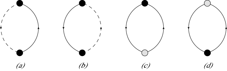
Figure 1: Diagrams with ${\bf A}$-linear contributions: (a) The solid line in upward direction represents the electron propagator $-G({\bf p+k/2},i\varepsilon_{n}+i\omega_{\lambda})$ and the broken line in downward direction represents $-G({\bf p+k/2}\leftarrow{\bf p-k/2},i\varepsilon_{n})$. Throughout the series of three Notes the Zeeman splitting is neglected so that the propagators for up-spin electrons and for down-spin electrons are degenerate. The upper black circle represents a component of $j^{e}_{\mu}({\bf k})$ where the momentum of the electron changes from ${\bf p+k/2}$ to ${\bf p-k/2}$ and the lower black circle represents a component of $j^{e}_{\nu}(0)$ where the momentum does not change. (b) The broken line in upward direction is $-G({\bf p+k/2}\leftarrow{\bf p-k/2},i\varepsilon_{n}+i\omega_{\lambda})$ and the solid line in downward direction is $-G({\bf p-k/2},i\varepsilon_{n})$. The upper black circle is $j^{e}_{\mu}({\bf k})$ and the lower black circle is $j^{e}_{\nu}(0)$. (c) The solid line in upward direction is $-G({\bf p+k/2},i\varepsilon_{n}+i\omega_{\lambda})$ and the solid line in downward direction is $-G({\bf p-k/2},i\varepsilon_{n})$. The upper black circle is $j^{e}_{\mu}({\bf k})$ and the lower gray circle is $-(e/m)\rho(-{\bf k})A_{\nu}$ where the momentum changes from ${\bf p-k/2}$ to ${\bf p+k/2}$. (d) The solid line in upward direction is $-G({\bf p},i\varepsilon_{n}+i\omega_{\lambda})$ and the solid line in downward direction is $-G({\bf p},i\varepsilon_{n})$. The upper gray circle is $-(e/m)\rho(0)A_{\mu}$, where the momentum does not change, and the lower gray circle is $j^{e}_{\nu}(0)$. The integral of this diagram in terms of ${\bf p}$ is odd under the variable change $p_{\nu}\rightarrow-p_{\nu}$ and vanishes so that (d) does not contribute to the conductivity.

The Feynman diagrams for the current-current correlation function in (7) are drawn in Fig. 1 where we only need the first order contributions in ${\bf A}$ to obtain the conductivity linear in ${\bf H}$ and the second order one has been neglected. The product of $j^{H}_{\mu}({\bf k})$ and $j^{H}_{\nu}(0)$ leads to four kinds of terms: (i) $j^{e}_{\mu}({\bf k})\cdot j^{e}_{\nu}(0)$, (ii) $j^{e}_{\mu}({\bf k})\cdot\rho(-{\bf k})A_{\nu}$, (iii) $\rho(0)A_{\mu}\cdot j^{e}_{\nu}(0)$, and (iv) $\rho(0)A_{\mu}\cdot\rho(-{\bf k})A_{\nu}$. In the case of (i) two current vertices can be connected by two ways as Figs. 1-(a) and (b) within the linear order of ${\bf A}$. In the cases of (ii) and (iii) one of the vertices is already proportional to ${\bf A}$ so that the vertices are connected by the electron propagator diagonal in momentum as Figs. 1-(c) and (d). The case (iv) is not considered here, because it is the second order contribution in ${\bf A}$.

Here $G({\bf p+k/2}\leftarrow{\bf p-k/2},i\varepsilon_{n})$ is the Fourier transform of the off-diagonal propagator in momentum variable

$$G({\bf p+k/2}\leftarrow{\bf p-k/2},\tau)=-\big{\langle}T_{\tau}\big{\{}c_{{\bf p+k/2}\sigma}(\tau)\ c_{{\bf p-k/2}\sigma}^{\dagger}\big{\}}\big{\rangle},$$ (15)

and evaluated by

$$G({\bf p+k/2}\leftarrow{\bf p-k/2},i\varepsilon_{n}) \fallingdotseq G({\bf p+k/2},i\varepsilon_{n})\cdot\big{(}-e{\bf v}_{\bf p}\cdot{\bf A}\big{)}\cdot G({\bf p-k/2},i\varepsilon_{n})$$

$$\fallingdotseq G({\bf p},i\varepsilon_{n})\cdot\big{(}-e{\bf v}_{\bf p}\cdot{\bf A}\big{)}\cdot G({\bf p},i\varepsilon_{n}),$$ (16)

which is the first order perturbation in terms of (12) in the limit of ${\bf k}\rightarrow 0$.

In order to obtain the conductivity proportional to the magnetic field defined in (5), which is linear in both ${\bf A}$ and ${\bf k}$, we have to extract the ${\bf k}$-linear contribution from the processes shown in Figs. 1-(a), (b), (c). A ${\bf k}$-linear contribution comes from the propagators diagonal in momentum variable ${\bf p\pm k/2}$ represented by the solid line. It also comes from $j^{e}_{\nu}(0)$ but does not from $j^{e}_{\mu}({\bf k})$.

The ${\bf k}$-linear part $\Phi^{e}_{(1)}(i\omega_{\lambda})$ of $\Phi_{xy}^{e}({\bf k},i\omega_{\lambda})$ is the summation of the ${\bf k}$-linear contributions, $\Phi_{(a)}$, $\Phi_{(b)}$, $\Phi_{(c)}$, which are extracted from the processes shown in Fig. 1-(a), (b), (c). Since $j^{e}_{x}({\bf k})$ leads to the factor $(e/m)p_{x}$, $j^{e}_{y}(0)$ to $(e/2m)k_{y}$, and $G({\bf p+k/2}\leftarrow{\bf p-k/2},i\varepsilon_{n})$ to $G({\bf p},i\varepsilon_{n})\cdot[-(e/m){\bf p}\cdot{\bf A}]\cdot G({\bf p},i\varepsilon_{n})$,

$$\Phi_{(a)}=-2T\sum_{n}\sum_{\bf p}{-1\over 2}\Big{(}{e\over m}\Big{)}^{3}p_{x}^{2}G({\bf p},i\varepsilon_{n}+i\omega_{\lambda})G({\bf p},i\varepsilon_{n})^{2}k_{y}A_{x},$$ (17)

where the product of the fermion-loop factor and the spin-degeneracy factor, -2, has been included. Since $j^{e}_{y}(0)$ leads to the factor $-(e/2m)k_{y}$,

$$\Phi_{(b)}=-2T\sum_{n}\sum_{\bf p}{1\over 2}\Big{(}{e\over m}\Big{)}^{3}p_{x}^{2}G({\bf p},i\varepsilon_{n}+i\omega_{\lambda})^{2}G({\bf p},i\varepsilon_{n})k_{y}A_{x}.$$ (18)

Since $\rho(-{\bf k})$ leads to the factor $-(e^{2}/m)A_{y}$, and $G({\bf p+k/2},i\varepsilon_{n}+i\omega_{\lambda})$ to $G({\bf p},i\varepsilon_{n}+i\omega_{\lambda})\cdot[+(1/2m){\bf p}\cdot{\bf k}]\cdot G({\bf p},i\varepsilon_{n}+i\omega_{\lambda})$, and $G({\bf p-k/2},i\varepsilon_{n})$ to $G({\bf p},i\varepsilon_{n})\cdot[-(1/2m){\bf p}\cdot{\bf k}]\cdot G({\bf p},i\varepsilon_{n})$,

$$\Phi_{(c)}=-2T\sum_{n}\sum_{\bf p}\Big{[}{-1\over 2} \Big{(}{e\over m}\Big{)}^{3}p_{x}^{2}G({\bf p},i\varepsilon_{n}+i\omega_{\lambda})^{2}G({\bf p},i\varepsilon_{n})k_{x}A_{y}$$

$$+{1\over 2} \Big{(}{e\over m}\Big{)}^{3}p_{x}^{2}G({\bf p},i\varepsilon_{n}+i\omega_{\lambda})G({\bf p},i\varepsilon_{n})^{2}k_{x}A_{y}\Big{]}.$$ (19)

Thus we obtain

$$\Phi_{(a)}+\Phi_{(b)}+\Phi_{(c)} =-{1\over 2}\Big{(}{e\over m}\Big{)}^{3}\big{(}k_{x}A_{y}-k_{y}A_{x}\big{)}T\sum_{n}\sum_{\bf p}p_{x}^{2}$$

$$\times\Big{[}G({\bf p},i\varepsilon_{n}+i\omega_{\lambda})G({\bf p},i\varepsilon_{n})^{2}-G({\bf p},i\varepsilon_{n}+i\omega_{\lambda})^{2}G({\bf p},i\varepsilon_{n})\Big{]}.$$ (20)

If we set ${\bf H}=(0,0,H)$ so that $H=i(k_{x}A_{y}-k_{y}A_{x})$, (20) leads to

$$\Phi^{e}_{(1)}(i\omega_{\lambda}) =-{H\over i}\Big{(}{e\over m}\Big{)}^{3}T\sum_{n}\sum_{\bf p}p_{x}^{2}$$

$$\times\Big{[}G({\bf p},i\varepsilon_{n}+i\omega_{\lambda})G({\bf p},i\varepsilon_{n})^{2}-G({\bf p},i\varepsilon_{n}+i\omega_{\lambda})^{2}G({\bf p},i\varepsilon_{n})\Big{]}.$$ (21)

Figure 2: Diagrams for a fixed gauge ${\bf A}=(A_{x},0,0)$: The left diagram corresponds to the one in Fig. 1-(a) and the right to Fig. 1-(b). The broken line represents the coupling to the magnetic field (12). (left) The solid line in upward direction is $-G({\bf p},i\varepsilon_{n}+i\omega_{\lambda})$. The downward process is the product $[-G({\bf p},i\varepsilon_{n})]\cdot[-(-J_{x}A_{x})]\cdot[-G({\bf p},i\varepsilon_{n})]$. The upper black circle is $J_{x}$ and the lower black circle is $(\partial J_{y}/\partial p_{y})k_{y}/2$. (right) The solid line in downward direction is $-G({\bf p},i\varepsilon_{n})$. The upward process is the product $[-G({\bf p},i\varepsilon_{n}+i\omega_{\lambda})]\cdot[-(-J_{x}A_{x})]\cdot[-G({\bf p},i\varepsilon_{n}+i\omega_{\lambda})]$. The upper black circle is $J_{x}$ and the lower black circle is $-(\partial J_{y}/\partial p_{y})k_{y}/2$. Here $J_{x}\equiv(e/m)p_{x}$ and $\partial J_{y}/\partial p_{y}\equiv e/m$.

If we choose the gauge ${\bf A}=(A_{x},0,0)$, we do not have to consider the contribution $\Phi_{(c)}$ of the diamagnetic current. Such a choice make the calculation simpler. The relevant processes leading to ${\bf H}$-linear contribution are summarized in Fig. 2. The expressions (17) and (18) are rewritten as

$$-{1\over 2}\Phi_{(a)}=T\sum_{n}\sum_{\bf p}J_{x}{\partial J_{y}\over\partial p_{y}}{k_{y}\over 2}G(i\varepsilon_{n})\big{(}-J_{x}A_{x}\big{)}G(i\varepsilon_{n})G(i\varepsilon_{n}+i\omega_{\lambda}),$$ (22)

$$-{1\over 2}\Phi_{(b)}=T\sum_{n}\sum_{\bf p}J_{x}{\partial J_{y}\over\partial p_{y}}\Big{(}-{k_{y}\over 2}\Big{)}G(i\varepsilon_{n})G(i\varepsilon_{n}+i\omega_{\lambda})\big{(}-J_{x}A_{x}\big{)}G(i\varepsilon_{n}+i\omega_{\lambda}),$$ (23)

where $J_{\mu}\equiv(e/m)p_{\mu}$ and $G(i\varepsilon_{n})\equiv G({\bf p},i\varepsilon_{n})$. In this case (21) is rewritten as

$$-{1\over 2}\Phi^{e}_{(1)}(i\omega_{\lambda}) ={H\over 2i}T\sum_{n}\sum_{\bf p}\big{(}J_{x}\big{)}^{2}{\partial J_{y}\over\partial p_{y}}$$

$$\times\Big{[}G(i\varepsilon_{n}+i\omega_{\lambda})G(i\varepsilon_{n})^{2}-G(i\varepsilon_{n}+i\omega_{\lambda})^{2}G(i\varepsilon_{n})\Big{]},$$ (24)

where the fermion-loop factor and the spin-degeneracy factor are moved to the left-hand side. Here $H=-ik_{y}A_{x}$.

In the following I adopt a shortcut calculation along [FEW] for

$$I^{e}(i\omega_{\lambda})\equiv-{1\over\beta}\sum_{n}X(i\varepsilon_{n})Y(i\varepsilon_{n}+i\omega_{\lambda}),$$ (25)

where $X(i\varepsilon_{n})\equiv[G({\bf p},i\varepsilon_{n})]^{a}$ and $Y(i\varepsilon_{n}+i\omega_{\lambda})\equiv[G({\bf p},i\varepsilon_{n}+i\omega_{\lambda})]^{b}$ with $a$ and $b$ being positive integers, because the calculation along §11 of [I] is cumbersome. By repeating the transformation which leads to (159) in [I] and neglecting the contributions from $C_{1}$ and $C_{4}$ we obtain

$$I^{e}(i\omega_{\lambda})\fallingdotseq\int_{-\infty}^{\infty}{d\epsilon\over 2\pi i}f(\epsilon)\Big{[}-X^{A}(\epsilon)Y^{R}(\epsilon+i\omega_{\lambda})+X^{A}(\epsilon-i\omega_{\lambda})Y^{R}(\epsilon)\Big{]},$$ (26)

where the first integrand is the contribution along $C_{2}$ and the second along $C_{3}$. The contours of the integral, $C_{1}$, $C_{2}$, $C_{3}$ and $C_{4}$, are defined in Fig. 5 of [I]. To calculate the DC conductivity we only need the $\omega$-linear contribution

$$I^{e}(\omega+i\delta)-I^{e}(i\delta) \fallingdotseq-\omega\int_{-\infty}^{\infty}{d\epsilon\over 2\pi i}f(\epsilon)\bigg{[}X^{A}(\epsilon){\partial Y^{R}(\epsilon)\over\partial\epsilon}+{\partial X^{A}(\epsilon)\over\partial\epsilon}Y^{R}(\epsilon)\bigg{]}$$

$$=-\omega\int_{-\infty}^{\infty}{d\epsilon\over 2\pi i}\Big{(}-{\partial f(\epsilon)\over\partial\epsilon}\Big{)}X^{A}(\epsilon)Y^{R}(\epsilon),$$ (27)

where we have employed the integration by parts. By the same approximation leading to (164) in [I], the application of (27) to (21) results in

$$\Phi^{e}_{(1)}(\omega+i\delta)-\Phi^{e}_{(1)}(i\delta)$$

$$\sim-i\omega{e^{3}\over m}\sum_{\bf p}v_{x}^{2}\Big{(}-{\partial f(\xi_{\bf p})\over\partial\xi_{\bf p}}\Big{)}\int_{-\infty}^{\infty}{d\epsilon\over 2\pi i}\Big{[}G^{A}({\bf p},\epsilon)G^{R}({\bf p},\epsilon)^{2}-G^{A}({\bf p},\epsilon)^{2}G^{R}({\bf p},\epsilon)\Big{]},$$ (28)

where

$$G^{R}({\bf p},\epsilon)={1\over\epsilon-\xi_{\bf p}+i/2\tau},\ \ \ \ \ \ \ \ \ \ G^{A}({\bf p},\epsilon)={1\over\epsilon-\xi_{\bf p}-i/2\tau},$$ (29)

which is the analytic continuation of the thermal propagator (13). The integral over $\epsilon$ is performed by evaluating the residue so that we finally obtain

$$\sigma_{xy} \equiv\lim_{\omega\rightarrow 0}\lim_{{\bf k}\rightarrow 0}{1\over i\omega}\big{[}\Phi_{xy}^{e}({\bf k},\omega+i\delta)-\Phi_{xy}^{e}({\bf k},i\delta)\big{]}$$

$$\sim 2{e^{3}\over m}H\sum_{\bf p}\Big{(}-{\partial f(\xi_{\bf p})\over\partial\xi_{\bf p}}\Big{)}v_{x}^{2}\tau^{2},$$ (30)

which coincides with the result of the Boltzmann transport (1) taking into account that ${\bf H}=(0,0,H)$ and ${\bf E}=(0,E,0)$.

The expectation value of the heat current ${\bf J}^{Q}$ is expressed as the linear response to electric field

$$J^{Q}_{\mu}({\bf k},\omega)=\sum_{\nu}{\tilde{\alpha}}_{\mu\nu}({\bf k},\omega)E_{\nu}({\bf k}\!=\!0,\omega),$$ (31)

with

$${\tilde{\alpha}}_{\mu\nu}({\bf k},\omega)={1\over i\omega}\big{[}\Phi_{\mu\nu}^{Q}({\bf k},\omega+i\delta)-\Phi_{\mu\nu}^{Q}({\bf k},i\delta)\big{]}.$$ (32)

As has been discussed in the above, in order to extract the contribution proportional to $H$, we only need the heat current $j^{Q}_{\mu}({\bf k})$ in the absence of the magnetic field so that only the difference between $\Phi^{e}_{\mu\nu}({\bf k},i\omega_{\lambda})$ and $\Phi^{Q}_{\mu\nu}({\bf k},i\omega_{\lambda})$ is the factor $(i\varepsilon_{n}+i\omega_{\lambda}/2)/e$ as in the case of §11 in [I].

By repeating the above shortcut calculation for

$$I^{Q}(i\omega_{\lambda})\equiv-{1\over\beta}\sum_{n}\Big{(}i\varepsilon_{n}+{i\omega_{\lambda}\over 2}\Big{)}X(i\varepsilon_{n})Y(i\varepsilon_{n}+i\omega_{\lambda}),$$ (33)

we obtain

$$I^{Q}(\omega+i\delta)\fallingdotseq\int_{-\infty}^{\infty}{d\epsilon\over 2\pi i}f(\epsilon)\Big{[}-\Big{(}\epsilon+{\omega\over 2}\Big{)}X^{A}(\epsilon)Y^{R}(\epsilon+\omega)+\Big{(}\epsilon-{\omega\over 2}\Big{)}X^{A}(\epsilon-\omega)Y^{R}(\epsilon)\Big{]}.$$ (34)

The $\omega$-linear contribution becomes

$$I^{Q}(\omega+i\delta)-I^{Q}(i\delta) \fallingdotseq-\omega\int_{-\infty}^{\infty}{d\epsilon\over 2\pi i}f(\epsilon)\bigg{\{}\epsilon\bigg{[}X^{A}(\epsilon){\partial Y^{R}(\epsilon)\over\partial\epsilon}+{\partial X^{A}(\epsilon)\over\partial\epsilon}Y^{R}(\epsilon)\bigg{]}+X^{A}(\epsilon)Y^{R}(\epsilon)\bigg{\}}$$

$$=-\omega\int_{-\infty}^{\infty}{d\epsilon\over 2\pi i}\Big{(}-{\partial f(\epsilon)\over\partial\epsilon}\Big{)}\ \epsilon\ X^{A}(\epsilon)Y^{R}(\epsilon),$$ (35)

by the integration by parts.

Thus the ${\bf k}$-linear part $\Phi^{Q}_{(1)}(i\omega_{\lambda})$ of $\Phi_{xy}^{Q}({\bf k},i\omega_{\lambda})$ is obtained as

$$\Phi^{Q}_{(1)}(\omega+i\delta)-\Phi^{Q}_{(1)}(i\delta)$$

$$\sim-i\omega{e^{2}\over m}\sum_{\bf p}v_{x}^{2}\Big{(}-{\partial f(\xi_{\bf p})\over\partial\xi_{\bf p}}\Big{)}\xi_{\bf p}\int_{-\infty}^{\infty}{d\epsilon\over 2\pi i}\Big{[}G^{A}({\bf p},\epsilon)G^{R}({\bf p},\epsilon)^{2}-G^{A}({\bf p},\epsilon)^{2}G^{R}({\bf p},\epsilon)\Big{]},$$ (36)

where we have pulled out the factor $-(\partial f(\epsilon)/\partial\epsilon)\cdot\epsilon$ from the integral over $\epsilon$ as in the case of §11 in [I]. Finally we obtain

$${\tilde{\alpha}}_{xy} \equiv\lim_{\omega\rightarrow 0}\lim_{{\bf k}\rightarrow 0}{1\over i\omega}\big{[}\Phi_{xy}^{Q}({\bf k},\omega+i\delta)-\Phi_{xy}^{Q}({\bf k},i\delta)\big{]}$$

$$\sim 2{e^{2}\over m}H\sum_{\bf p}\Big{(}-{\partial f(\xi_{\bf p})\over\partial\xi_{\bf p}}\Big{)}v_{x}^{2}\tau^{2}\xi_{\bf p},$$ (37)

which coincides with the result of the Boltzmann transport (2).

4 GL Transport

The linearized GL transport theory gives

$$\sigma_{xy}={e^{2}\over 48d}{\tau_{2}\over\tau_{1}}{h\over\epsilon^{2}},$$ (38)

and

$$\alpha_{xy}={|e|\over 4\pi d}{h\over\epsilon},$$ (39)

where $h\equiv 2|e|H\xi_{0}^{2}$. The derivation of these results shall be discussed by the non-perturbational treatment of the magnetic field in the third Note.

5 Cooper-Pair Transport: AL Process

The calculations for electrons in §3 are translated into those for Cooper pairs straightforwardly. The contribution of the left diagram in Fig. 3 is

$$\Phi_{(a)}=T\sum_{m}\sum_{\bf q}{\tilde{\Delta}}_{x}^{e}{\partial{\tilde{\Delta}}_{y}^{e}\over\partial q_{y}}{k_{y}\over 2}L(i\omega_{m})\big{(}-{\tilde{\Delta}}_{x}^{e}A_{x}\big{)}L(i\omega_{m})L(i\omega_{m}+i\omega_{\lambda}),$$ (40)

which corresponds to (22) and that of the right diagram is

$$\Phi_{(b)}=T\sum_{m}\sum_{\bf q}{\tilde{\Delta}}_{x}^{e}{\partial{\tilde{\Delta}}_{y}^{e}\over\partial q_{y}}\Big{(}-{k_{y}\over 2}\Big{)}L(i\omega_{m})L(i\omega_{m}+i\omega_{\lambda})\big{(}-{\tilde{\Delta}}_{x}^{e}A_{x}\big{)}L(i\omega_{m}+i\omega_{\lambda}),$$ (41)

which corresponds to (23) where ${\tilde{\Delta}}_{\mu}^{e}\equiv 4eN(0)\xi_{0}^{2}q_{\mu}$ and $L(i\omega_{m})\equiv L({\bf q},i\omega_{m})$.

Figure 3: AL process for a fixed gauge ${\bf A}=(A_{x},0,0)$: These diagrams correspond to those in Fig. 2. The broken line represents the coupling to the magnetic field (12). (left) The wavy line in right-side is $-L({\bf q},i\omega_{m}+i\omega_{\lambda})$. The left-side process is the product $[-L({\bf q},i\omega_{m})]\cdot[-(-{\tilde{\Delta}}^{e}_{x}A_{x})]\cdot[-L({\bf q},i\omega_{m})]$. The upper black circle is ${\tilde{\Delta}}^{e}_{x}$ and the lower black circle is $(\partial{\tilde{\Delta}}^{e}_{y}/\partial q_{y})k_{y}/2$. (right) The wavy line in left-side is $-L({\bf q},i\omega_{m})$. The right-side process is the product $[-L({\bf q},i\omega_{m}+i\omega_{\lambda})]\cdot[-(-{\tilde{\Delta}}^{e}_{x}A_{x})]\cdot[-L({\bf q},i\omega_{m}+i\omega_{\lambda})]$. The upper black circle is ${\tilde{\Delta}}^{e}_{x}$ and the lower black circle is $-(\partial{\tilde{\Delta}}^{e}_{y}/\partial q_{y})k_{y}/2$. Here ${\tilde{\Delta}}^{e}_{x}\equiv 4eN(0)\xi_{0}^{2}q_{x}$ and $\partial{\tilde{\Delta}}^{e}_{y}/\partial q_{y}\equiv 4eN(0)\xi_{0}^{2}$.

Thus (24) is translated into

$$\Phi^{e}_{(1)}(i\omega_{\lambda}) ={H\over 2i}T\sum_{m}\sum_{\bf q}\big{(}{\tilde{\Delta}}_{x}^{e}\big{)}^{2}{\partial{\tilde{\Delta}}_{y}^{e}\over\partial q_{y}}$$

$$\times\Big{[}L(i\omega_{m}+i\omega_{\lambda})L(i\omega_{m})^{2}-L(i\omega_{m}+i\omega_{\lambda})^{2}L(i\omega_{m})\Big{]}.$$ (42)

This result is rewritten as

$$\Phi^{e}_{(1)}(i\omega_{\lambda})=32{H\over i}\big{(}e\xi_{0}^{2}\big{)}^{3}\sum_{\bf q}q_{x}^{2}{\tilde{I}}^{e}(i\omega_{\lambda}),$$ (43)

with

$${\tilde{I}}^{e}(i\omega_{\lambda})\equiv T\sum_{m}\Big{[}{\tilde{L}}(i\omega_{m}+i\omega_{\lambda})^{2}{\tilde{L}}(i\omega_{m})-{\tilde{L}}(i\omega_{m}+i\omega_{\lambda}){\tilde{L}}(i\omega_{m})^{2}\Big{]},$$ (44)

where $L(i\omega_{m})\equiv-{\tilde{L}}(i\omega_{m})/N(0)$. Analytical continuation of this discrete summation becomes

$${\tilde{I}}^{e}(\omega+i\delta)=\int_{-\infty}^{\infty}{dx\over\pi}n(x)\Big{\{}\big{[}R(+)^{2}-A(-)^{2}\big{]}{\rm Im}R-\big{[}R(+)-A(-)\big{]}{\rm Im}R^{2}\Big{\}},$$ (45)

where

$$R={1\over\eta-i\tau_{0}x},\ \ \ \ \ \ \ \ \ \ A={1\over\eta+i\tau_{0}^{*}x},$$ (46)

$$R(+)={1\over\eta-i\tau_{0}(x+\omega)},\ \ \ \ \ \ \ \ \ \ A(-)={1\over\eta+i\tau_{0}^{*}(x-\omega)}.$$ (47)

Here $\tau_{0}$ is complex, $\tau_{0}\equiv\tau_{1}+i\tau_{2}$, and $\tau_{1}\gg|\tau_{2}|$. The $\omega$-linear contribution is evaluated as

$${\tilde{I}}^{e}(\omega+i\delta)-{\tilde{I}}^{e}(i\delta) \fallingdotseq\omega\int_{-\infty}^{\infty}{dx\over\pi}n(x)\Big{\{}\Big{[}2R{\partial R\over\partial x}+2A{\partial A\over\partial x}\Big{]}{\rm Im}R-\Big{[}{\partial R\over\partial x}+{\partial A\over\partial x}\Big{]}{\rm Im}R^{2}\Big{\}}$$

$$=\omega\int_{-\infty}^{\infty}{dx\over 2\pi i}n(x)\big{(}R-A\big{)}\Big{\{}R{\partial R\over\partial x}+A{\partial A\over\partial x}-R{\partial A\over\partial x}-A{\partial R\over\partial x}\Big{\}},$$ (48)

where ${\rm Im}R=(R-A)/2i$ and ${\rm Im}R^{2}=(R+A)(R-A)/2i$. Employing the high-temperature expansion, $n(x)\fallingdotseq T/x$,

$${\tilde{I}}^{e}(\omega+i\delta)-{\tilde{I}}^{e}(i\delta)\fallingdotseq\omega T\cdot J,$$ (49)

with

$$J\equiv\int_{-\infty}^{\infty}{dx\over 2\pi i}{R-A\over x}\Big{\{}R{\partial R\over\partial x}+A{\partial A\over\partial x}-R{\partial A\over\partial x}-A{\partial R\over\partial x}\Big{\}}.$$ (50)

Here we have picked up

$${R-A\over ix}=(\tau_{0}^{*}+\tau_{0})RA,$$ (51)

in the integrand, because ${\rm Im}L^{R}(x)/x$ is proportional to the Lorentz function in $x$ and basic quantity. Using

$${\partial R\over\partial x}=i\tau_{0}R^{2},\ \ \ \ \ \ \ \ \ \ {\partial A\over\partial x}=-i\tau_{0}^{*}A^{2},$$ (52)

we obtain

$$J=\int_{-\infty}^{\infty}{dx\over 2\pi i}(\tau_{0}^{*}+\tau_{0})RA\big{\{}-\tau_{0}R^{3}+\tau_{0}^{*}A^{3}\big{\}}.$$ (53)

The integral is evaluated by the residue so that

$$J=-i{\tau_{0}^{*}\tau_{0}(\tau_{0}-\tau_{0}^{*})\over(\tau_{0}^{*}+\tau_{0})^{2}}{1\over\eta^{4}}\fallingdotseq{\tau_{2}\over 2}{1\over\eta^{4}}.$$ (54)

Therefore

$$\Phi^{e}_{(1)}(\omega+i\delta)-\Phi^{e}_{(1)}(i\delta)\fallingdotseq 16{H\over i}e^{3}\omega T\tau_{2}\sum_{\bf q}{\xi_{0}^{6}q_{x}^{2}\over(\epsilon+\xi_{0}^{2}{\bf q}^{2})^{4}},$$ (55)

and this leads to

$$\sigma_{xy}=-16He^{3}T\tau_{2}\sum_{\bf q}{\xi_{0}^{6}q_{x}^{2}\over(\epsilon+\xi_{0}^{2}{\bf q}^{2})^{4}}.$$ (56)

In 2D the ${\bf q}$-summation is performed as

$$\sum_{\bf q}{\xi_{0}^{4}q_{x}^{2}\over(\epsilon+\xi_{0}^{2}{\bf q}^{2})^{4}}={1\over 8\pi d}\int_{0}^{\infty}dx{x\over(x+\epsilon)^{4}}={1\over 48\pi d}{1\over\epsilon^{2}}.$$ (57)

Finally we obtain (38) by using $\tau_{1}=\pi/8T$.

Only the difference between $\Phi^{e}_{\mu\nu}({\bf k},i\omega_{\lambda})$ and $\Phi^{Q}_{\mu\nu}({\bf k},i\omega_{\lambda})$ is the factor $(i\omega_{m}+i\omega_{\lambda}/2)/2e$ as has been discussed in §3 so that we readily obtain

$$\Phi^{Q}_{(1)}(i\omega_{\lambda})=32{H\over i}\big{(}e\xi_{0}^{2}\big{)}^{3}\sum_{\bf q}q_{x}^{2}{1\over 2e}{\tilde{I}}^{Q}(i\omega_{\lambda}),$$ (58)

with

$${\tilde{I}}^{Q}(i\omega_{\lambda})\equiv T\sum_{m}\Big{(}i\omega_{m}+{i\omega_{\lambda}\over 2}\Big{)}\Big{[}{\tilde{L}}(i\omega_{m}+i\omega_{\lambda})^{2}{\tilde{L}}(i\omega_{m})-{\tilde{L}}(i\omega_{m}+i\omega_{\lambda}){\tilde{L}}(i\omega_{m})^{2}\Big{]}.$$ (59)

Analytical continuation of this discrete summation becomes

$${\tilde{I}}^{Q}(\omega+i\delta) =\int_{-\infty}^{\infty}{dx\over\pi}n(x)\Big{(}x+{\omega\over 2}\Big{)}\Big{\{}R(+)^{2}\cdot{\rm Im}R-R(+)\cdot{\rm Im}R^{2}\Big{\}}$$

$$+\int_{-\infty}^{\infty}{dx\over\pi}n(x)\Big{(}x-{\omega\over 2}\Big{)}\Big{\{}{\rm Im}R^{2}\cdot A(-)-{\rm Im}R\cdot A(-)^{2}\Big{\}}$$

$$\equiv{\tilde{I}}_{1}^{Q}(\omega+i\delta)+{\tilde{I}}_{2}^{Q}(\omega+i\delta),$$ (60)

where

$${\tilde{I}}_{1}^{Q}(\omega+i\delta)=\int_{-\infty}^{\infty}{dx\over\pi}n(x)\ x\ \Big{\{}\big{[}R(+)^{2}-A(-)^{2}\big{]}{\rm Im}R-\big{[}R(+)-A(-)\big{]}{\rm Im}R^{2}\Big{\}},$$ (61)

$${\tilde{I}}_{2}^{Q}(\omega+i\delta)={\omega\over 2}\int_{-\infty}^{\infty}{dx\over\pi}n(x)\Big{\{}\big{[}R(+)^{2}+A(-)^{2}\big{]}{\rm Im}R-\big{[}R(+)+A(-)\big{]}{\rm Im}R^{2}\Big{\}}.$$ (62)

In the following the imaginary part of $\tau_{0}$ is neglected: $\tau_{0}^{*}=\tau_{0}$ or $\tau_{2}=0$. Employing the high-temperature expansion, $n(x)\fallingdotseq T/x$, we obtain

$${\tilde{I}}_{1}^{Q}(\omega+i\delta)-{\tilde{I}}_{1}^{Q}(i\delta) \fallingdotseq{T\over\pi}\omega\int_{-\infty}^{\infty}dx\Big{\{}\Big{[}2R{\partial R\over\partial x}+2A{\partial A\over\partial x}\Big{]}{\rm Im}R-\Big{[}{\partial R\over\partial x}+{\partial A\over\partial x}\Big{]}{\rm Im}R^{2}\Big{\}}$$

$$={T\over\pi}\omega\int_{-\infty}^{\infty}dx{\tau_{0}\over 2}\big{(}R+A\big{)}\big{(}R-A\big{)}^{3}=0,$$ (63)

$${\tilde{I}}_{2}^{Q}(\omega+i\delta)-{\tilde{I}}_{2}^{Q}(i\delta) \fallingdotseq{T\over 2\pi}\omega\int_{-\infty}^{\infty}{dx\over x}\Big{\{}\Big{(}R^{2}+A^{2}\Big{)}{\rm Im}R-\Big{(}R+A\Big{)}{\rm Im}R^{2}\Big{\}}$$

$$={T\over 2\pi}\omega\int_{-\infty}^{\infty}dx\big{(}-2\tau_{0}\big{)}R^{2}A^{2}$$

$$=-{T\over 2}\omega{1\over\eta^{3}}.$$ (64)

Therefore

$$\Phi^{Q}_{(1)}(\omega+i\delta)-\Phi^{Q}_{(1)}(i\delta)\fallingdotseq 8He^{2}i\omega T\sum_{\bf q}{\xi_{0}^{6}q_{x}^{2}\over(\epsilon+\xi_{0}^{2}{\bf q}^{2})^{3}}.$$ (65)

In 2D the ${\bf q}$-summation is performed as

$$\sum_{\bf q}{\xi_{0}^{4}q_{x}^{2}\over(\epsilon+\xi_{0}^{2}{\bf q}^{2})^{3}}={1\over 8\pi d}\int_{0}^{\infty}dx{x\over(x+\epsilon)^{3}}={1\over 16\pi d}{1\over\epsilon}.$$ (66)

Finally we obtain (39) via

$${\tilde{\alpha}}_{xy}=T{e^{2}\over 2\pi d}H\xi_{0}^{2}{1\over\epsilon}.$$ (67)

The calculations in the absence of the magnetic field are also performed in the same manner. The integral (207) in [I] with real $\tau_{0}$ is evaluated as

$$I^{e}(\omega+i\delta)-I^{e}(i\delta) \fallingdotseq{1\over N(0)^{2}}{T\over\pi}\omega\int_{-\infty}^{\infty}dx\Big{[}{\partial R\over\partial x}-{\partial A\over\partial x}\Big{]}{R-A\over 2ix}$$

$$={1\over N(0)^{2}}{T\over\pi}i\omega\tau_{0}^{2}\int_{-\infty}^{\infty}dx\big{(}R^{2}+A^{2}\big{)}RA$$

$$={T\over 2N(0)^{2}}i\omega\tau_{0}{1\over\eta^{3}}.$$ (68)

The integral (216) in [I] with complex $\tau_{0}$ is evaluated as

$$I^{Q}(\omega+i\delta)-I^{Q}(i\delta) \fallingdotseq{1\over N(0)^{2}}{T\over\pi}\omega\int_{-\infty}^{\infty}dx\Big{[}{\partial R\over\partial x}-{\partial A\over\partial x}\Big{]}{R-A\over 2i}$$

$$+{1\over N(0)^{2}}{T\over\pi}{\omega\over 2}\int_{-\infty}^{\infty}dx\big{(}R-A\big{)}{R-A\over 2ix},$$ (69)

to give (220) in [I].

6 Remarks

The sections of Exercise and Acknowledgements are common to [I] so that I do not repeat here. Some typographic errors in [I] are listed below.

• The thermodynamic relation in p. 11 should be $dQ=dU-\mu dN$.

• The electric field in (68) and (78) should be $E_{\nu}({\bf k}\!=\!0,\omega)$.

• The factor $e$ in the first line of (73) should be $e/m$.

• In Fig. 5 the subscript $\lambda$ for the lower cut $C_{\lambda}$ has dropped by the font-error at $\mathsf{arXiv}$.

• In the footnote 47 the first term in the right-hand side of the complex GL equation should be $(1+ic_{0}){\tilde{\Psi}}$.

Appendix

The linear response theory for the DC Hall conductivity of the Dirac fermion in 2+1 space-time dimensions is reviewed. One focus is the Chern-Simons effective action for the gauge field. Another is the exact formula by Ishikawa and Matsuyama.

A1. Introduction

The topological nature of the DC Hall conductivity in 2+1 space-time dimensions was intensively discussed in 1980’s in the context of the quantum Hall effect. The discussion based on the Dirac fermion was a major topic in those days. In the study of topological insulators there is a revival of interest in the description by the Dirac fermion in these days. Thus this review of the linear response theory for the DC Hall conductivity of the Dirac fermion might be useful to beginners in the 21st century.

In the section 2 the details of the perturbational derivation of the Chern-Simons effective action for the gauge field at zero temperature are given.

In the section 3 a brief discussion on the exact formula at zero temperature by Ishikawa and Matsuyama is given.

A2. Chern-Simons action

We consider the coupled system of the Dirac fermion and the gauge field in 2+1 space-time dimensions. By tracing out the fermion field we obtain the Chern-Simons effective action for the gauge field.

The Lagrangian density for the Dirac fermion is given by

$${\cal L}={\bar{\psi}}(i\gamma_{\mu}\partial^{\mu}-m)\psi,$$ (70)

where ${\bar{\psi}}=\psi^{\dagger}\gamma^{0}$ and $\gamma_{\mu}\partial^{\mu}=\gamma_{0}\partial_{0}-\gamma_{1}\partial_{1}-\gamma_{2}\partial_{2}$.

Since

$$\gamma_{0}=\sigma_{z},\ \ \ \gamma_{1}=i\sigma_{x},\ \ \ \gamma_{2}=i\sigma_{y},$$ (71)

the properties of the gamma matrices are those of the Pauli matrices.

The free propagator of the Dirac fermion is given by the matrix

$$G(p)={1\over{\not{p}}-m+i\delta}={{\not{p}}+m\over p^{2}-m^{2}+i\delta},$$ (73)

where $\not{p}=\gamma_{\mu}p^{\mu}=p_{0}\gamma_{0}-p_{1}\gamma_{1}-p_{2}\gamma_{2}$, $p^{2}=p_{0}^{2}-p_{1}^{2}-p_{2}^{2}$ and $\delta=+0$. The component proportional to $\gamma_{0}$ is

$${1\over 2}\Big{(}{1\over p_{0}-E_{\bf p}+i\delta^{\prime}}+{1\over p_{0}+E_{\bf p}-i\delta^{\prime}}\Big{)},$$ (74)

where $E_{\bf p}=\sqrt{p_{1}^{2}+p_{2}^{2}+m^{2}}$ with ${\bf p}=(p_{1},p_{2})$. In my notation $m>0$ and $E_{\bf p}>0$.

The coupling between the fermion and the gauge fields is given by the interaction Lagrangian

$${\cal L}_{\rm int}=-ej_{\mu}(x)A^{\mu}(x),$$ (75)

where

$$j_{\mu}(x)={\bar{\psi}}(x)\gamma_{\mu}\psi(x).$$ (76)

The effective action $S$ for the gauge field is obtained as

$$iS={i^{2}\over 2!}\int{d^{3}x}\int{d^{3}y}A^{\mu}(x)\big{\langle}0\big{|}T\big{\{}J_{\mu}(x)J_{\nu}(y)\big{\}}\big{|}0\big{\rangle}A^{\nu}(y),$$ (77)

within the second order perturbation in ${\cal L}_{\rm int}$. Assuming the translational invariance,

$$\big{\langle}0\big{|}T\big{\{}J_{\mu}(x)J_{\nu}(y)\big{\}}\big{|}0\big{\rangle}=i\Pi_{\mu\nu}(x-y),$$ (78)

and introducing the Fourier transform

$$\Pi_{\mu\nu}(x-y)=\int{d^{3}q\over(2\pi)^{3}}\Pi_{\mu\nu}(q)\exp[-iq(x-y)],$$ (79)

$S$ is expressed as

$$S=-{1\over 2}\int{d^{3}q\over(2\pi)^{3}}A^{\mu}(-q)\Pi_{\mu\nu}(q)A^{\nu}(q),$$ (80)

where

$$\Pi_{\mu\nu}(q)=ie^{2}\int{d^{3}p\over(2\pi)^{3}}{\rm tr}\big{[}\gamma_{\mu}G\big{(}p+{q\over 2}\big{)}\gamma_{\nu}G\big{(}p-{q\over 2}\big{)}\big{]},$$ (81)

in the perturbational calculation.

The Chern-Simons action is the $q$-linear contribution of (80). The integrand of (81) is

$${{\rm tr}\big{[}\gamma_{\mu}({\not{p}}+{\not{q}}/2+m)\gamma_{\nu}({\not{p}}-{\not{q}}/2+m)\big{]}\over\big{[}(p+q/2)^{2}-m^{2}+i\delta\big{]}\big{[}(p-q/2)^{2}-m^{2}+i\delta\big{]}},$$ (82)

The $q$-linear contributions from $(p+q/2)^{2}$ and $(p-q/2)^{2}$ cancel out. The $q$-linear contribution from the trace over the gamma matrix is

$${m\over 2}{\rm tr}\big{[}\gamma_{\mu}{\not{q}}\gamma_{\nu}\big{]}-{m\over 2}{\rm tr}\big{[}\gamma_{\mu}\gamma_{\nu}{\not{q}}\big{]}=m{\rm tr}\big{[}\gamma_{\mu}\gamma_{\lambda}\gamma_{\nu}\big{]}q^{\lambda}.$$ (83)

Thus

$$S=-{i\over 2}\kappa\int{d^{3}q\over(2\pi)^{3}}A^{\mu}(-q)q^{\lambda}A^{\nu}(q)\epsilon_{\mu\lambda\nu},$$ (84)

where

$$\kappa=e^{2}\int{d^{3}p\over(2\pi)^{3}}{-2im\over(p^{2}-m^{2}+i\delta)^{2}}=-2ime^{2}\int_{0}^{\infty}{|{\bf p}|d|{\bf p}|\over 2\pi}I(|{\bf p}|),$$ (85)

with

$$I(|{\bf p}|)=\int_{-\infty}^{\infty}{dp_{0}\over 2\pi}{1\over(p_{0}-E_{\bf p}+i\delta^{\prime})^{2}(p_{0}+E_{\bf p}-i\delta^{\prime})^{2}},$$ (86)

and $|{\bf p}|=\sqrt{p_{1}^{2}+p_{2}^{2}}$. The integral $I(|{\bf p}|)$ is evaluated by the contour consisting of the real axis and the semi-circle with infinitely large radius in the upper half of the complex $p_{0}$-plane and results in

$$I(|{\bf p}|)={i\over 4}E_{\bf p}^{-3}.$$ (87)

As the contribution from the occupied branch $-E_{\bf p}$ we obtain

$$\kappa={me^{2}\over 4\pi}\int_{-\infty}^{-m}{-\epsilon_{\bf p}d\epsilon_{\bf p}\over(-\epsilon_{\bf p})^{3}}={e^{2}\over 4\pi}.$$ (88)

With this $\kappa$ the effective action $S$ in the coordinate representation becomes

$$S={\kappa\over 2}\int{d^{3}x}A^{\mu}(x)\partial^{\lambda}A^{\nu}(x)\epsilon_{\mu\lambda\nu},$$ (89)

where $\partial^{\lambda}=\partial/\partial x_{\lambda}$.

The expectation value of the electric current is given as

$$\overline{J_{1}(x)}={\delta S\over\delta A^{1}(x)}=\kappa\big{(}\partial^{2}A^{0}-\partial^{0}A^{2}\big{)}=\kappa E^{2}.$$ (90)

Namely,

$$\overline{J^{1}(x)}=\sigma_{xy}E^{2},$$ (91)

with the DC Hall conductivity

$$\sigma_{xy}=-{e^{2}\over 4\pi}.$$ (92)

In the presence of the chemical potential $\mu$ the Lagrangian density becomes

$${\cal L}+\mu\psi^{\dagger}\psi={\cal L}+\mu{\bar{\psi}}\gamma^{0}\psi,$$ (93)

since $(\gamma_{0})^{2}=I$. Then the pole of the propagator in the complex $p_{0}$-plane is located at

$$p_{0}+\mu=\epsilon_{\bf p}-i\delta^{\prime}{\rm sign}(\epsilon_{\bf p}-\mu),$$ (94)

where $\epsilon_{\bf p}=E_{\bf p}$ or $\epsilon_{\bf p}=-E_{\bf p}$. We only pick up the contribution of the pole in the upper plane.

When $-m<\mu<m$, the branch $-E_{\bf p}$ is fully occupied so that $\kappa$ ie equal to (88).

When $\mu<-m$, the branch $-E_{\bf p}$ is partially occupied so that

$$\kappa={me^{2}\over 4\pi}\int_{-\infty}^{\mu}{-\epsilon_{\bf p}d\epsilon_{\bf p}\over(-\epsilon_{\bf p})^{3}}={e^{2}\over 4\pi}{m\over|\mu|}.$$ (95)

When $m<\mu$, the branch $-E_{\bf p}$ is fully occupied and the branch $+E_{\bf p}$ is partially occupied so that

$$\kappa={me^{2}\over 4\pi}\biggl{(}\int_{-\infty}^{-m}{-\epsilon_{\bf p}d\epsilon_{\bf p}\over(-\epsilon_{\bf p})^{3}}-\int_{m}^{\mu}{\epsilon_{\bf p}d\epsilon_{\bf p}\over\epsilon_{\bf p}^{3}}\biggr{)}={e^{2}\over 4\pi}{m\over|\mu|}.$$ (96)

The absolute value of the Hall conductivity $\kappa$ shows Mt. Fuji shape as a function of the chemical potential $\mu$.

A3. Ishikawa-Matsuyama formula

As discussed above the DC Hall conductivity is determined by the $q$-linear contribution of

$${\rm tr}\big{[}\gamma_{\mu}G(p+q)\gamma_{\nu}G(p)\big{]}.$$ (97)

In the following we consider the case with zero chemical potential. Since

$${1\over{\not{p}}+{\not{q}}-m}={1\over{\not{p}}-m}-{1\over{\not{p}}-m}{\not{q}}{1\over{\not{p}}-m}+\cdot\cdot\cdot,$$ (98)

the $q$-linear contribution is

$$-{\rm tr}\big{[}\gamma_{\mu}G(p)\gamma_{\lambda}G(p)\gamma_{\nu}G(p)\big{]}q^{\lambda}.$$ (99)

This is the result for free fermions.

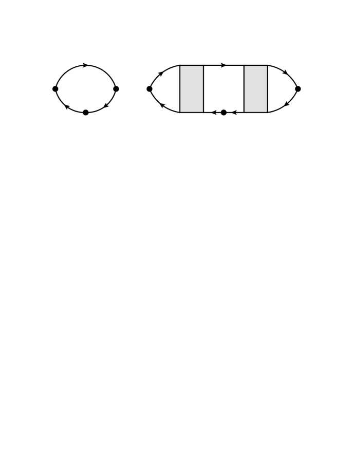
Figure 4: (Left): Insulator and (Right): Metal.

In the case of interacting fermions the propagator $G(p)$ is renormalized into ${\tilde{G}}(p)$ and $\gamma$ into $\Gamma$ so that the DC Hall conductivity is determined by

$$-{\rm tr}\big{[}\Gamma_{\mu}{\tilde{G}}(p)\Gamma_{\lambda}{\tilde{G}}(p)\Gamma_{\nu}{\tilde{G}}(p)\big{]}q^{\lambda},$$ (100)

whose diagrammatic representation is given as Fig. 4-(Left). The Ward identity tells us

$$\Gamma_{\mu}={\partial{\tilde{G}}(p)^{-1}\over\partial p^{\mu}},$$ (101)

so that (100) becomes

$$-{\rm tr}\biggl{[}{\partial{\tilde{G}}(p)^{-1}\over\partial p^{\mu}}{\tilde{G}}(p){\partial{\tilde{G}}(p)^{-1}\over\partial p^{\lambda}}{\tilde{G}}(p){\partial{\tilde{G}}(p)^{-1}\over\partial p^{\nu}}{\tilde{G}}(p)\biggr{]}q^{\lambda}.$$ (102)

If the renormalized propagator is given as ${\tilde{G}}(p)=Z_{2}G(p)$ with a constant $Z_{2}$, (102) becomes

$$-{\rm tr}\biggl{[}{\partial G(p)^{-1}\over\partial p^{\mu}}G(p){\partial G(p)^{-1}\over\partial p^{\lambda}}G(p){\partial G(p)^{-1}\over\partial p^{\nu}}G(p)\biggr{]}q^{\lambda}.$$ (103)

Since

$$\gamma_{\mu}={\partial G(p)^{-1}\over\partial p^{\mu}},$$ (104)

(103) is equal to (99). Namely, the DC Hall conductivity is not renormalized by the interaction.

This absence of interaction-renormalization occurs for insulators where the energy spectrum has the mass gap. On the other hand, in the case of metals where the chemical potential is out of the mass gap and in the continuum, we have to consider the effect of damping whose diagrammatic representation is given as Fig. 4-(Right). The damping relevant to the DC conductivity is dominantly determined by the process with zero-energy excitation at the chemical potential. In the case of insulators such an excitation is absent so that the conductivity is not renormalized.

A4. Remarks

The success of the Ishikawa-Matsuyama formula results from the cancelation between the self-energy and vertex corrections. On the other hand, the FLEX approximation violates such a cancelation as criticized in arXiv:1406.5831.