Bayesian matching of unlabeled marked point sets using random fields, with an application to molecular alignment

Abstract

Statistical methodology is proposed for comparing unlabeled marked point sets, with an application to aligning steroid molecules in chemoinformatics. Methods from statistical shape analysis are combined with techniques for predicting random fields in spatial statistics in order to define a suitable measure of similarity between two marked point sets. Bayesian modeling of the predicted field overlap between pairs of point sets is proposed, and posterior inference of the alignment is carried out using Markov chain Monte Carlo simulation. By representing the fields in reproducing kernel Hilbert spaces, the degree of overlap can be computed without expensive numerical integration. Superimposing entire fields rather than the configuration matrices of point coordinates thereby avoids the problem that there is usually no clear one-to-one correspondence between the points. In addition, mask parameters are introduced in the model, so that partial matching of the marked point sets can be carried out. We also propose an adaptation of the generalized Procrustes analysis algorithm for the simultaneous alignment of multiple point sets. The methodology is illustrated with a simulation study and then applied to a data set of 31 steroid molecules, where the relationship between shape and binding activity to the corticosteroid binding globulin receptor is explored.

T1Supported by an EPSRC/University of Nottingham studentship and a Leverhulme Research Fellowship.

, and

1 Introduction

In many application areas it is of interest to compare marked point sets, where measurements (marks) are available at various point locations, and often the configurations of points are unlabeled in the sense that there is no natural correspondence between the points in each configuration. The task of comparing unlabeled marked point sets has been of recent interest in statistical shape analysis, for example, Green and Mardia (2006), Dryden, Hirst and Melville (2007) and Schmidler (2007). As opposed to these previous approaches, our method does not aim to model point correspondences. Instead, the objects are compared by assuming a common underlying reference field which gives rise to the spatial distribution of the marks.

One example where the alignment of unlabeled marked point sets is of practical importance comes from the fields of structural bioinformatics and chemoinformatics, where it is of great interest to align molecules. However, the task is often very difficult. The motivating application in this paper is a data set comprising 31 steroid molecules which bind to the corticosteroid binding globulin (CBG) receptor. For each molecule, the Cartesian coordinates of the atom positions, as well as the associated van der Waals radii, and the partial atomic charge values at the atom positions are provided. Here the marks at each point (atom) are either the van der Waals radii or the partial charges. The steroids fall into three activity classes with respect to their binding activity to the CBG receptor [Good, So and Richards (1993)], and the main objective in this application is to compare the molecules in order to obtain the common features in each of the three groups and to examine whether these features are associated with the type of binding activity.

We consider a simple model under which spatial prediction of a reference field is carried out using the observed marks in each configuration. A measure of similarity between the two predicted fields is then used to describe the similarity, taking into account an unknown transformation between the point sets which gave rise to the actually observed point coordinates. The parsimonious model does not attempt to model accurately all aspects of the molecules in our application. It is rather used to develop a Bayesian algorithm based on Markov chain Monte Carlo (MCMC) simulations for matching, which is demonstrated to work well in our applications. In this setting it is also possible to introduce additional parameters (mask vectors) which allow for the fact that only part of the point sets may be similar. By determining and aligning only the similar parts of the given point sets, a meaningful comparison can be carried out.

In Section 2 we motivate and describe our newly developed measure of similarity for comparing unlabeled marked point sets. The Bayesian framework for the pairwise alignment and similarity calculation is introduced in Section 3. An extension of this methodology to the simultaneous alignment of multiple point sets is described in Section 3.3. In Section 4 we carry out simulation studies in two and three dimensions to validate our method. In Section 5 we apply our methods to the steroids data and assess the results with respect to their chemical relevance. Finally, Section 6 concludes the paper with a discussion.

2 Similarity measures using spatial prediction

2.1 Random field model

The starting point for our model is an underlying reference random field $\{Z(\mathbf{x})\dvtx\mathbf{x}\in\mathbb{R}^{m}\}$ which is assumed to be second-order stationary with a constant mean $E(Z(\mathbf{x}))=\mu$ and a positive definite covariance function $\sigma(\mathbf{h})=\operatorname{Cov}(Z(\mathbf{x}),Z(\mathbf{x}+\mathbf{h}))=\sigma(-\mathbf{h})$. Consider two marked point sets $A$ and $B$, say, which are $z$-values at point locations in the field given by $\mathbf{x}^{\prime\mathrm{A}}_{i}\in\mathbb{R}^{m},i=1,\ldots,k_{A}$, and $\mathbf{x}^{\prime\mathrm{B}}_{j}\in\mathbb{R}^{m},j=1,\ldots,k_{B}$. In a vector representation, the marked point sets $A$ and $B$ can therefore be written as

$$\mathbf{z}^{\mathrm{A}}=\{z^{\mathrm{A}}(\mathbf{x}^{\prime\mathrm{A}}_{1}),\ldots,z^{\mathrm{A}}(\mathbf{x}^{\prime\mathrm{A}}_{k_{\mathrm{A}}})\},\qquad\mathbf{z}^{\mathrm{B}}=\{z^{\mathrm{B}}(\mathbf{x}^{\prime\mathrm{B}}_{1}),\ldots,z^{\mathrm{B}}(\mathbf{x}^{\prime\mathrm{B}}_{k_{\mathrm{B}}})\},$$

respectively. Note that the relative position of $A$ and $B$ as given by $\{\mathbf{x}^{\prime\mathrm{A}}_{1},\ldots,\allowbreak\mathbf{x}^{\prime\mathrm{A}}_{k_{\mathrm{A}}}\}$ and $\{\mathbf{x}^{\prime\mathrm{B}}_{1},\ldots,\mathbf{x}^{\prime\mathrm{B}}_{k_{\mathrm{B}}}\}$ is special because the spatial distribution of the marks within each point set and also the spatial distribution of the joint set of marks $\mathbf{z}^{\mathrm{AB}}=\{z^{\mathrm{A}}(\mathbf{x}^{\prime\mathrm{A}}_{1}),\ldots,z^{\mathrm{A}}(\mathbf{x}^{\prime\mathrm{A}}_{k_{\mathrm{A}}}),z^{\mathrm{B}}(\mathbf{x}^{\prime\mathrm{B}}_{1}),\ldots,z^{\mathrm{B}}(\mathbf{x}^{\prime\mathrm{B}}_{k_{\mathrm{B}}})\}$ directly reflect the properties of $\{Z(\mathbf{x})\dvtx\mathbf{x}\in\mathbb{R}^{m}\}$. In that sense it can be regarded as the true relative position.

However, in real-life data sets the given marked point sets are often provided in arbitrary locations, that is, before being recorded each point set is transformed to new locations $\mathbf{x}^{\mathrm{A}}_{i}=\Phi_{\mathrm{A}}(\mathbf{x}^{\prime\mathrm{A}}_{i}),i=1,\ldots,k_{\mathrm{A}}$, and $\mathbf{x}^{\mathrm{B}}_{j}=\Phi_{\mathrm{B}}(\mathbf{x}^{\prime\mathrm{B}}_{j}),j=1,\ldots,k_{\mathrm{B}}$, where $\Phi_{\mathrm{A}}\dvtx\mathbb{R}^{m}\to\mathbb{R}^{m}$ and $\Phi_{\mathrm{B}}\dvtx\mathbb{R}^{m}\to\mathbb{R}^{m}$ are unknown transformation functions which are assumed to be 1–1 and onto. Hence, the inverse transformations $\Phi_{\mathrm{A}}^{-1}$ and $\Phi_{\mathrm{B}}^{-1}$ exist and satisfy $\Phi_{\mathrm{A}}^{-1}\{\Phi_{\mathrm{A}}(\mathbf{x})\}=\mathbf{x}=\Phi_{\mathrm{A}}\{\Phi_{\mathrm{A}}^{-1}(\mathbf{x})\}$ and $\Phi_{\mathrm{B}}^{-1}\{\Phi_{\mathrm{B}}(\mathbf{x})\}=\mathbf{x}=\Phi_{\mathrm{B}}\{\Phi_{\mathrm{B}}^{-1}(\mathbf{x})\}$, respectively.

The basic inference problem we consider in this paper can now be formulated as follows: if we are given the two marked point sets $A$ and $B$ with $\mathbf{z}^{\mathrm{A}}$ recorded at locations $\{\mathbf{x}^{\mathrm{A}}_{1},\ldots,\mathbf{x}^{\mathrm{A}}_{k_{\mathrm{A}}}\}$ and $\mathbf{z}^{\mathrm{B}}$ recorded at locations $\{\mathbf{x}^{\mathrm{B}}_{1},\ldots,\mathbf{x}^{\mathrm{B}}_{k_{\mathrm{B}}}\}$, can we measure how similar they are, taking into account the unknown transformation $\Phi=\Phi_{\mathrm{A}}\Phi_{\mathrm{B}}^{-1}$ from $B$ to $A$? The method involves aligning the point sets by estimating the transformation parameters in $\Phi$.

The particular choice of the set of potential transformations will depend on the application. In our case the marked point sets are the partial charges or the van der Waals radii of the steroid molecules which are recorded in arbitrary positions and orientations. As steroid molecules in general are rigid (the word is derived from “stereos”${}={}$“rigid” in Greek), we consider the rigid body transformations of translation and rotation, that is,

$$\Phi(\mathbf{x})=\bolds\Gamma\mathbf{x}+\bolds\gamma,\qquad\bolds\Gamma\in\operatorname{SO}(m),\bolds\gamma\in\mathbb{R}^{m},$$ (1)

where the space of special orthogonal matrices $\operatorname{SO}(m)$ contains the rotation matrices which satisfy $\bolds\Gamma^{T}\bolds\Gamma=\bolds\Gamma\bolds\Gamma^{T}=\mathbf{I}_{m}$ and $|\bolds\Gamma|=1$. Other more complicated transformations could be used, such as when more dynamic aspects of molecule shape need to be taken into account. For example, movement around rotatable bonds could be added if desired in other applications. The choice of $\mu$ and $\sigma(\mathbf{h})$ in the random field will also depend on the application.

In order to estimate the transformation parameters in $\Phi$, we first consider predicting the underlying reference field $Z(\mathbf{x})$ using each point set separately. A similarity measure is then defined which measures how close the two predicted fields are in a certain relative position. Finally, we can estimate the unknown transformation by maximizing the similarity measure or, alternatively, by developing a statistical model based on the similarity measure.

2.2 Kriging

In order to predict the underlying reference random field from each point set, we consider simple kriging [e.g., Cressie (1993), page 110] which assumes the mean field $\mu=0$. For the steroid molecules with partial charge or van der Waals radius marks, it makes sense to fix $\mu=0$, so that a long way from the molecular skeleton the predicted field is zero. We will use a sample variogram to help suggest an appropriate covariance function.

Consider a general marked point set $\mathbf{z}=\{z(\mathbf{x}_{1}),\ldots,z(\mathbf{x}_{k})\}$. If simple kriging is used to predict the value of the underlying random field $\{Z(\mathbf{x})\dvtx\mathbf{x}\in\mathbb{R}^{m}\}$ at a location of interest $\mathbf{x}_{0}$, say, a weighted average of the form $\hat{Z}(\mathbf{x}_{0})=\sum_{i=1}^{k}u_{i}z(\mathbf{x}_{i})$ is sought so as to minimize the prediction mean squared error $\operatorname{PMSE}(\mathbf{u})=\mathrm{E}[(\hat{Z}(\mathbf{x}_{0})-Z(\mathbf{x}_{0}))^{2}]$ with respect to the weight vector $\mathbf{u}=(u_{1},\allowbreak\ldots,u_{k})^{T}$. Given the observed values in $\mathbf{z}$, the corresponding system of equations has the solution $\mathbf{u}=\bolds\Sigma^{-1}\bolds\sigma$, and the predicted value for $Z(\mathbf{x}_{0})$ is given by $\hat{Z}(\mathbf{x}_{0})=\bolds\sigma(\mathbf{x}_{0})^{T}\bolds\Sigma^{-1}\mathbf{z}=\mathbf{u}^{T}\mathbf{z}$, where $\bolds\sigma(\mathbf{x}_{0})=(\sigma(\mathbf{x}_{1}-\mathbf{x}_{0}),\ldots,\sigma(\mathbf{x}_{k}-\mathbf{x}_{0}))^{T}$ and $(\bolds\Sigma)_{ij}=\sigma(\mathbf{x}_{i}-\mathbf{x}_{j})$, $1\leq i,j\leq k$. For a general location $\mathbf{x}$ this yields the predicted field

$$\hat{Z}(\mathbf{x})=\mathbf{z}^{T}\bolds\Sigma^{-1}\bolds\sigma(\mathbf{x})=\sum_{i=1}^{k}w_{i}\sigma(\mathbf{x}_{i}-\mathbf{x}),$$ (2)

where the weight vector $\mathbf{w}=(w_{1},\ldots,w_{k})^{T}=\bolds\Sigma^{-1}\mathbf{z}$ is optimal in terms of minimizing the PMSE if the underlying assumptions are met. Note that in some applications it may not be appropriate to assume $\mu=0$, in which case one would work with the mean corrected field $Z(\mathbf{x})-\mu$, where $\mu$ is either known or estimated using generalized least squares from each marked point set.

Using (2) and based on the observed data vectors $\mathbf{z}^{\mathrm{A}}$ and $\mathbf{z}^{\mathrm{B}}$, we can obtain a different prediction of the underlying reference random field from each of the two marked point sets $A$ and $B$, and the resulting predicted fields $\hat{Z}_{\mathrm{A}}(\mathbf{x})$ and $\hat{Z}_{\mathrm{B}}(\mathbf{x})$ then need to be compared.

2.3 Function similarity and the Kernel Carbo index

In order to measure the similarity of the predicted fields $\hat{Z}_{\mathrm{A}}(\mathbf{x})$ and $\hat{Z}_{\mathrm{B}}(\mathbf{x})$, we require a metric space where the notion of similarity can be defined by means of the corresponding inner product. A commonly used metric space for functions is the space of Lebesgue square-integrable functions $L_{2}$, where the inner product has the form

$$\langle f,g\rangle_{L_{2}}=\int f(\mathbf{x})g(\mathbf{x})\,d\mathbf{x}.$$ (3)

Based on (3), an intuitive measure of similarity between two functions $f$ and $g$ can be formulated which does not depend on the scales of $f$ and $g$, that is,

$$R_{\mathrm{fg}}=\frac{\int f(\mathbf{x})g(\mathbf{x})\,d\mathbf{x}}{(\int f(\mathbf{x})^{2}\,d\mathbf{x})^{1/2}(\int g(\mathbf{x})^{2}\,d\mathbf{x})^{1/2}}=\frac{\langle f,g\rangle_{L_{2}}}{(\langle f,f\rangle_{L_{2}}\langle g,g\rangle_{L_{2}})^{1/2}},$$

and so $R_{\mathrm{fg}}=1$ if $f=cg$, where $c>0$ is a positive constant, and $R_{\mathrm{fg}}=-1$ if $c<0$. Note that $R_{\mathrm{fg}}$ is a generalization of Pearson’s correlation coefficient for comparing two functions. Also note that, in general, calculation of $R_{\mathrm{fg}}$ would involve numerical integration over the domain, which may be computationally demanding.

An alternative metric space for functions is a reproducing kernel Hilbert space (RKHS) that, for a given reproducing kernel, can easily be constructed and is much simpler and quicker to use in practice. This alternative is very useful for our model because the covariance function $\sigma$ of the reference random field can be viewed as a reproducing kernel on $\mathbb{R}^{m}\times\mathbb{R}^{m}$ due to the properties of a general covariance function (e.g., symmetric and positive definite). Hence, the corresponding RKHS exists [Aronszajn (1950)] and can be written as $\mathcal{H}_{\sigma}=\{f|f(\mathbf{x})=\sum_{i=1}^{k_{\mathrm{A}}}\alpha_{i}\sigma(\mathbf{x}_{i}^{\mathrm{A}}-\mathbf{x})\}$. In this space the inner product of $f(\mathbf{x})=\sum_{i=1}^{k_{\mathrm{A}}}\alpha_{i}\sigma(\mathbf{x}_{i}^{\mathrm{A}}-\mathbf{x})\in\mathcal{H}_{\sigma}$ and $g(\mathbf{x})=\sum_{j=1}^{k_{\mathrm{B}}}\beta_{j}\sigma(\mathbf{x}_{j}^{\mathrm{B}}-\mathbf{x})\in\mathcal{H}_{\sigma}$ has the form

$$\langle f,g\rangle_{\mathcal{H}_{\sigma}}=\sum_{i=1}^{k_{\mathrm{A}}}\sum_{j=1}^{k_{\mathrm{B}}}\alpha_{i}\beta_{j}\sigma(\mathbf{x}_{i}^{\mathrm{A}}-\mathbf{x}_{j}^{\mathrm{B}}),$$

which can be evaluated without expensive numerical integration.

Note that we can view the kriging predictor (2) as a member of $\mathcal{H}_{\sigma}$, and, hence, we can use the RKHS inner product $\langle\cdot,\cdot\rangle_{\mathcal{H}_{\sigma}}$ to measure the similarity between the predicted fields of $A$ and $B$. Let $\hat{Z}_{\mathrm{A}}(\mathbf{x})=\sum_{i=1}^{k_{\mathrm{A}}}w^{\mathrm{A}}_{i}\sigma(\mathbf{x}_{i}^{\mathrm{A}}-\mathbf{x})$ and $\hat{Z}_{\mathrm{B}}(\mathbf{x})=\sum_{j=1}^{k_{\mathrm{B}}}w^{\mathrm{B}}_{j}\sigma(\Phi(\mathbf{x}_{j}^{\mathrm{B}})-\mathbf{x})$ denote the predicted fields of the marked point sets $A$ and $B$ in the relative position defined by $\Phi=\Phi_{A}\Phi_{B}^{-1}$. The similarity measure we propose in this paper has the form

$$C_{\mathrm{AB}}(\bolds\phi)=\frac{\langle\hat{Z}_{\mathrm{A}},\hat{Z}_{\mathrm{B}}\rangle_{\mathcal{H}_{\sigma}}}{\|\hat{Z}_{\mathrm{A}}\|_{\mathcal{H}_{\sigma}}\|\hat{Z}_{\mathrm{B}}\|_{\mathcal{H}_{\sigma}}},$$ (4)

where $\|\hat{Z}_{\mathrm{M}}\|^{2}_{\mathcal{H}_{\sigma}}=\langle\hat{Z}_{\mathrm{M}},\hat{Z}_{\mathrm{M}}\rangle_{\mathcal{H}_{\sigma}}$ $(M\in\{A,B\})$, and $\bolds\phi$ denotes the parameter vector of the unknown transformation $\Phi$. The numerator term measures the “overlap” of the fields (in a certain relative position), whereas the denominator is a transformation invariant normalizing constant which ensures that $C_{\mathrm{AB}}(\bolds\phi)\in[-1,1]$. Note that (4) can also be interpreted as the cosine of the angle between the two predicted fields in a certain relative position.

We shall call the above similarity function the “Kernel Carbo function,” as it is a modification of a similarity function proposed by Carbo, Leyda and Arnau (1980) in the context of field-based molecular alignment. The fields considered in that original paper are the electron densities of the two molecules under study, and the similarity was defined in terms of the $L_{2}$ inner product given in (3). As both fields in our setting are members of the RKHS $\mathcal{H}_{\sigma}$, the Carbo similarity function can be “kernelized” by replacing $\langle\cdot,\cdot\rangle_{L_{2}}$ with $\langle\cdot,\cdot\rangle_{\mathcal{H}_{\sigma}}$, which has the advantage that calculating (4) does not require evaluation of overlap integrals over $\mathbb{R}^{m}$ for any choice of positive definite covariance function.

For the reproducing kernel we shall consider the istropic Matérn covariance function, where the covariance of the field between any pair of points $\mathbf{x},\mathbf{y}$ is given by

$$\sigma(\mathbf{x}-\mathbf{y})=\frac{1}{2^{\nu-1}\Gamma(\nu)}\biggl{(}\frac{2\nu^{1/2}\|\mathbf{x}-\mathbf{y}\|}{\rho}\biggr{)}^{\nu}K_{\nu}\biggl{(}\frac{2\nu^{1/2}\|\mathbf{x}-\mathbf{y}\|}{\rho}\biggr{)}.$$ (5)

This provides a flexible family of stationary covariance functions [Stein (1999), page 31]. With this particular parameterization [e.g., Handcock and Wallis (1994)], $\rho$ is a range parameter and $\nu$ determines the smoothness of the random field. Moreover, $K_{\nu}(\cdot)$ is the modified Bessel function of the third kind of order $\nu$ and $\Gamma(\cdot)$ is the Gamma function. Note that $\nu\to\infty$ corresponds to the Gaussian covariance function

$$\sigma(\mathbf{x}-\mathbf{y})=\exp\{-\|\mathbf{x}-\mathbf{y}\|^{2}/\rho^{2}\},$$ (6)

and in this particular case the $L_{2}$-Carbo index of our predicted fields could be calculated analytically.

Optimizing (4) with respect to the transformation parameters yields the “Kernel Carbo index”

$$C(A,B)=\sup_{\bolds\phi}C_{\mathrm{AB}}(\bolds\phi)=\sup_{\bolds\phi}\frac{\langle\hat{Z}_{\mathrm{A}},\hat{Z}_{\mathrm{B}}\rangle_{\mathcal{H}_{\sigma}}}{\|\hat{Z}_{\mathrm{A}}\|_{\mathcal{H}_{\sigma}}\|\hat{Z}_{\mathrm{B}}\|_{\mathcal{H}_{\sigma}}},$$ (7)

in which configuration $B$ is transformed (by the relative transformation function $\Phi$) to be as similar as possible to configuration $A$. In the case (1) where the rigid body transformations in $\mathbb{R}^{m}$ are considered, the parameter vector $\bolds\phi$ contains $m(m-1)/2$ Euler angles for rotation and $m$ translation parameters, and in this case the Kernel Carbo index is invariant under the rigid body transformations of $A$ and $B$.

Note that the optimization in (7) is not straightforward in practice due to local maxima. As an approximation to using the Kernel Carbo index in (7), we will therefore propose a Bayesian model and find the value of the similarity index (4) at the maximum a posteriori (MAP) estimates of the transformation parameters. Also note that, in situations where a dissimilarity rather than a similarity measure is required, (4) can be uniquely mapped into the appropriate codomain using

$$D_{\mathrm{AB}}(\bolds\phi)=\frac{1-C_{\mathrm{AB}}(\bolds\phi)}{1+C_{\mathrm{AB}}(\bolds\phi)}\in[0,\infty),$$ (8)

and applying the same transformation to (7) or its MAP equivalent then yields a transformation invariant dissimilarity index between two marked point sets.

2.4 Masks

In many applications it is of interest to match parts of objects rather than the entire configurations. Our steroids application is one such example because only a part of each molecule may fit into the binding pocket of the common receptor and is hence relevant for the binding mechanism. As a tool for matching only parts of the given configurations, we consider a set of masks (indicator parameters) which signify if individual points are included in the predicted field or not. The masks therefore allow for the possibility that only parts of the structures match, whereas other parts may have been generated by different underlying reference fields or may be largely affected by noise.

From now on we will just consider rigid body transformations between the point sets, with rotation matrix $\bolds\Gamma$ and translation vector $\bolds\gamma$, although, as mentioned above, the approach can be extended to other transformations.

Let $\bolds\lambda_{\mathrm{M}}\,{=}\,(\lambda^{\mathrm{M}}_{1},\ldots,\lambda^{\mathrm{M}}_{k_{M}})^{T}$ be the mask vector for point set $M$ ($M\,{\in}\,\{A,B\}$). Each entry of the mask vector is an indicator function, that is, $\lambda^{\mathrm{M}}_{i}\in\{0,1\}$ which determines if the $i$th point of set $M$ is considered to contribute to the matching parts $(\lambda^{\mathrm{M}}_{i}=1)$ or not $(\lambda^{\mathrm{M}}_{i}=0)$, $i=1,\ldots,k_{M}$. Taking the mask vector into account, the predicted version of the common reference field based on $M$ then has the form $\hat{Z}_{\mathrm{M}}(\mathbf{x};\bolds\lambda_{\mathrm{M}})=\sum_{i\dvtx\lambda^{\mathrm{M}}_{i}=1}w^{\mathrm{M}}_{i}(\bolds\lambda_{\mathrm{M}})\sigma(\mathbf{x}_{i}^{\mathrm{M}}-\mathbf{x})$, and the resulting partial Kernel Carbo function for two masked fields $\hat{Z}_{\mathrm{A}}(\mathbf{x};\bolds\lambda_{\mathrm{A}})$ and $\hat{Z}_{\mathrm{B}}(\mathbf{x};\bolds\lambda_{\mathrm{B}})$ in a certain relative position becomes

$$C_{\mathrm{AB}}(\bolds\Gamma,\bolds\gamma,\bolds\lambda_{\mathrm{A}},\bolds\lambda_{\mathrm{B}})=\sum_{i\dvtx\lambda^{\mathrm{A}}_{i}=1}\sum_{j\dvtx\lambda^{\mathrm{B}}_{j}=1}\tilde{w}^{\mathrm{A}}_{i}(\bolds\lambda_{\mathrm{A}})\tilde{w}^{\mathrm{B}}_{j}(\bolds\lambda_{\mathrm{B}})\sigma\bigl{(}\mathbf{x}_{i}^{\mathrm{A}}-(\bolds\Gamma\mathbf{x}_{j}^{\mathrm{B}}+\bolds\gamma)\bigr{)},$$ (9)

where the tilde indicates that the kriging weights are normalized by the corresponding term in the normalizing constant, that is, $\tilde{w}^{\mathrm{M}}_{i}(\bolds\lambda_{\mathrm{M}})=w^{\mathrm{M}}_{i}(\bolds\lambda_{\mathrm{M}})/\allowbreak N_{\mathrm{M}}(\bolds\lambda_{\mathrm{M}})$, with $N_{\mathrm{M}}(\bolds\lambda_{\mathrm{M}})=\|\hat{Z}_{\mathrm{M}}(\mathbf{x};\bolds\lambda_{\mathrm{M}})\|_{\mathcal{H}_{\sigma}}$. The partial Kernel Carbo index can then be obtained by maximizing (9) over the transformation and mask parameters.

Optimizing the similarity measure (9) over all possible subsets is very challenging due to the combinatorial nature of the search space. Instead we use a Bayesian model to obtain the MAP estimates of the similarity transformations and masks and then evaluate (9) at the MAP, which approximates the maximization of (9). Rather than trying to develop a realistic probabilistic model for the data, we therefore view the Bayesian model and the resulting MCMC scheme as a practical approach for generating an algorithm to match two spatial point patterns. Also, apart from transforming the problem into a more tractable one, the Bayesian setting allows the introduction of prior information about the parameters which will be useful, for example, to prevent excessive masking.

3 Bayesian pairwise alignment of marked point sets

3.1 Likelihood

With the assumption that the similar parts of the two point sets are noisy pointwise observations of the same underlying reference field, we define the likelihood for the two marked point sets $\mathbf{z}^{\mathrm{A}}=\{z^{\mathrm{A}}(\mathbf{x}^{\mathrm{A}}_{1}),\ldots,z^{\mathrm{A}}(\mathbf{x}^{\mathrm{A}}_{k_{\mathrm{A}}})\}$ and $\mathbf{z}^{\mathrm{B}}=\{z^{\mathrm{B}}(\mathbf{x}^{\mathrm{B}}_{1}),\ldots,z^{\mathrm{B}}(\mathbf{x}^{\mathrm{B}}_{k_{\mathrm{B}}})\}$ in the relative position defined by $\bolds\Gamma$ and $\bolds\gamma$ as

$$L(\mathbf{z}^{\mathrm{A}},\mathbf{z}^{\mathrm{B}}|\bolds\theta,\bolds\gamma,\bolds\lambda_{\mathrm{A}},\bolds\lambda_{\mathrm{B}},\tau)\propto\tau\exp(-\tau D_{\mathrm{AB}}(\bolds\Gamma,\bolds\gamma,\bolds\lambda_{\mathrm{A}},\bolds\lambda_{\mathrm{B}})),$$ (10)

where $\bolds\theta$ denotes the vector of the Euler angles which specifies a rotation matrix $\bolds\Gamma(\bolds\theta)$, $\bolds\gamma$ denotes a displacement vector between $A$ and $B$, $\tau\in\mathbb{R}^{+}$ is a precision parameter, and $D_{\mathrm{AB}}(\bolds\Gamma,\bolds\gamma,\bolds\lambda_{\mathrm{A}},\bolds\lambda_{\mathrm{B}})$ is the dissimilarity function based on (8) and (9). Here, the mask vectors play a similar role as the labeling matrices in Green and Mardia (2006), Dryden, Hirst and Melville (2007) and Schmidler (2007), except in our framework there is no need to establish correspondences between points in $A$ and $B$. Instead, the mask vectors are defined separately for each point set. The pairwise correspondence does not need be estimated because all possible pairs of atoms are considered in the model, and the pairs are weighted according to how far apart they are during the matching.

Note that if $\tau$ is fixed, the likelihood is maximized at the same rotation, translation and mask parameter estimates that give the maximum value of the partial Kriged Carbo index (9). This, and the fact that it performed well in pilot simulations, provides the motivation for the use of this likelihood. Other choices include the half-normal likelihood

$$L(A,B|\bolds\theta,\bolds\gamma,\bolds\lambda_{\mathrm{A}},\bolds\lambda_{\mathrm{B}},\tau)\propto\tau^{1/2}\exp(-\tau D^{2}_{\mathrm{AB}}(\bolds\Gamma,\bolds\gamma,\bolds\lambda_{\mathrm{A}},\bolds\lambda_{\mathrm{B}})),$$

which is less accommodating of outliers but might be preferable in some situations.

3.2 Prior distributions and posterior sampling

We do not have any prior information about the rigid body parameters $\bolds\theta$ and $\bolds\gamma$ so that they are treated as uniformly distributed on $\operatorname{SO}(m)$ and on a large bounded region in $\mathbb{R}^{m}$, respectively. The uniform distribution on $\operatorname{SO}(m)$ is determined by the probability measure which is invariant under the group action. In the two-dimensional case, $f_{U}(\bolds\theta)\propto 1$. For $m=3$, the appropriate density with respect to the Lebesgue measure depends on the parametrization of $\operatorname{SO}(3)$, and in this paper we use the Euler angles in the so-called $x$-convention where

$$\bolds\Gamma(\bolds\theta)=\pmatrix{\cos\theta_{3}\!&\!\sin\theta_{3}\!&\!0\cr-\sin\theta_{3}\!&\!\cos\theta_{3}\!&\!0\cr 0\!&\!0\!&\!1\!}\!\pmatrix{1\!&\!0\!&\!0\cr 0\!&\!\cos\theta_{2}\!&\!\sin\theta_{2}\cr 0\!&\!-\sin\theta_{2}\!&\!\cos\theta_{2}}\!\pmatrix{\cos\theta_{1}\!&\!\sin\theta_{1}\!&\!0\cr-\sin\theta_{1}\!&\!\cos\theta_{1}\!&\!0\cr 0\!&\!0\!&\!1}.$$

In that case, $f_{U}(\bolds\theta)\propto\cos(\theta_{2})$ and with the domains $-\pi\leq\theta_{1},\theta_{3}<\pi$ and $-\pi/2\leq\theta_{2}<\pi/2$, every $\bolds\Gamma\in\operatorname{SO}(3)$ is uniquely determined apart from a singularity at $\theta_{2}=-\pi/2$.

To prevent the situation where only very few points are used in the field comparison, we introduce a (fixed) penalty parameter $\zeta\geq 0$ and a (fixed) interaction parameter $\zeta_{I}\geq 0$ to define the joint prior density of the mask vectors as

$$\pi(\bolds\lambda_{\mathrm{A}},\bolds\lambda_{\mathrm{B}}|\zeta,\zeta_{I})\propto\zeta^{\sum_{i}\lambda_{i}^{\mathrm{A}}+\sum_{i}\lambda_{i}^{\mathrm{B}}}+\zeta_{I}^{\sum_{i\stackrel{{\scriptstyle\mathrm{A}}}{{\sim}}j}|\lambda_{i}^{\mathrm{A}}-\lambda_{j}^{\mathrm{A}}|+\sum_{i\stackrel{{\scriptstyle\mathrm{B}}}{{\sim}}j}|\lambda_{i}^{\mathrm{B}}-\lambda_{j}^{\mathrm{B}}|},$$

where $i\stackrel{{\scriptstyle\mathrm{M}}}{{\sim}}j$ means that points $i$ and $j$ are neighbors within $M$ ($M\in\{A,B\}$), for example, if $\|\mathbf{x}^{\mathrm{M}}_{i}-\mathbf{x}^{\mathrm{M}}_{j}\|<\delta$. Note that the dimensions of $\bolds\lambda_{\mathrm{A}}\in\{0,1\}^{k_{\mathrm{A}}}$ and $\bolds\lambda_{\mathrm{B}}\in\{0,1\}^{k_{\mathrm{B}}}$ are fixed. The penalty parameter $\zeta$ inherently comprises prior assumptions about the extent of the matching parts of $A$ and $B$, with higher $\zeta$ indicating more prior matching points. Also, if the interaction parameter $\zeta_{I}$ is strictly greater than 1, this indicates clustering so that nearby points within a point set are expected to be included (or excluded) together in the matching. Thus, a large positive $\zeta_{I}$ would be used when we wish to encourage contiguous regions to be included in the matching, although we shall use $\zeta_{I}=1$ in our applications.

With the further assumptions that the precision parameter is Gamma distributed a priori, that is, $\tau\sim\Gamma(\alpha,\beta)$, and that all unknown parameters are independent a priori, the joint posterior conditioned on the given data is

$$\pi(\bolds\theta,\bolds\gamma,\bolds\lambda_{\mathrm{A}},\bolds\lambda_{\mathrm{B}},\tau|\mathbf{z}^{A},\mathbf{z}^{B},\alpha,\beta,\zeta,\zeta_{I})$$

$$\qquad\propto\tau^{\alpha}\exp\bigl{\{}-\tau\bigl{(}D_{\mathrm{AB}}(\bolds\Gamma,\bolds\gamma,\bolds\lambda_{\mathrm{A}},\bolds\lambda_{\mathrm{B}})+\beta\bigr{)}\bigr{\}}\cdot\pi(\bolds\lambda_{\mathrm{A}},\bolds\lambda_{\mathrm{B}}|\zeta,\zeta_{I})\cdot f_{U}(\bolds\theta).$$

Note that this can be regarded as a mixture model over $\{0,1\}^{k_{\mathrm{A}}}\times\{0,1\}^{k_{\mathrm{B}}}$.

We use MCMC to sample from the posterior distribution. The resulting point estimates for the rigid body parameters and the mask vectors can then be substituted into $D_{\mathrm{AB}}(\bolds\Gamma,\bolds\gamma,\bolds\lambda_{\mathrm{A}},\bolds\lambda_{\mathrm{B}})$ to yield a point estimate of the dissimilarity measure

$$\hat{D}_{\mathrm{AB}}=D_{\mathrm{AB}}(\hat{\bolds\Gamma},\hat{\bolds\gamma},\hat{\bolds\lambda}_{\mathrm{A}},\hat{\bolds\lambda}_{\mathrm{B}}).$$ (11)

In the MCMC scheme, $\tau$ is updated with a Gibbs step. Updated versions of the other parameters are obtained in four blocks, each using a Metropolis–Hastings step. For the rigid body parameters, we use independent normal proposals, and a proposal distribution for the masks vectors $\bolds\lambda_{\mathrm{A}}$ and $\bolds\lambda_{\mathrm{B}}$ can be obtained by choosing an entry at random and then switching its value from zero to one or vice versa.

The algorithm we use ensures that the defined Markov chain is irreducible, aperiodic and positive recurrent, and, hence, after a large number of iterations the simulated value is approximately generated from the posterior distribution. Due to the symmetry of the proposal distributions, convergence to and sampling from the limiting distribution in practice thereby results in an approximate stochastic minimization of the dissimilarity term, and this behavior can be emphasized by choosing a prior distribution with a large mean for $\tau$. In fact, if one is mainly interested in obtaining point estimates of the model parameters which provide a good superposition, simulated annealing [Kirkpatrick, Gelatt and Vecchi (1983)] can be employed so that the MCMC algorithm simulates from $\pi(\bolds\theta,\bolds\gamma,\bolds\lambda_{\mathrm{A}},\bolds\lambda_{\mathrm{B}},\tau|A,B,\alpha,\beta,\zeta,\zeta_{I})^{1/T},$ where $T>0$ is slowly reduced deterministically.

As with any MCMC scheme for a complicated high-dimensional problem, there is a possibility that the chain will become stuck in a local region of maximum posterior probability, and our application is no exception. Hence, judicious use of proposal distributions is required to escape such regions, for example, the use of occasional large proposal variances.

Note that the partial Kriged Carbo index and the Bayesian model are symmetric in terms of which point set is denoted as $A$ and which point set is denoted as $B$. However, for a practical implementation one of the points sets is chosen as $B$ and transformed to be as close as possible to the other point set $A$. As our method is simulation based, slightly different estimates will be obtained in matching $A$ to $B$ and then $B$ to $A$. Hence, in our application we carry out both matches and then take an appropriately symmetrized average of the estimated distance measures, for example, their geometric mean.

3.3 Multiple alignment

In the multiple alignment problem, the objective is to simultaneously superimpose a set of $n$ marked point sets $M_{1},\ldots,M_{n}$. Previous approaches to this problem include Dryden, Hirst and Melville (2007) and Ruffieux and Green (2009). Here, we adapt the generalized Procrustes analysis (GPA) algorithm for discrete landmark data [e.g., Dryden and Mardia (1998), page 90] to our field-based approach. In the classical GPA context it is of interest to find an alignment of the given objects which minimizes the sum of their pairwise squared distances. A similar goodness-of-fit criterion for the multiple superposition of $n$ predicted masked fields can be formulated in terms of their overall similarity as

$$C(\bolds\theta,\bolds\gamma,\bolds\lambda)$$

$$\qquad=\sum_{i=1}^{n-1}\sum_{j=i+1}^{n}\biggl{\{}\sum_{l\dvtx\lambda^{i}_{l}=1}\sum_{l^{\prime}\dvtx\lambda^{j}_{l^{\prime}}=1}\tilde{w}^{i}_{l}(\bolds\lambda_{i})\tilde{w}^{j}_{l^{\prime}}(\bolds\lambda_{j})\sigma\bigl{(}(\bolds\Gamma_{i}\mathbf{x}_{l}^{i}+\bolds\gamma_{i})$$ (12)

$$\hskip 213.5pt{}-(\bolds\Gamma_{j}\mathbf{x}_{l^{\prime}}^{j}+\bolds\gamma_{j})\bigr{)}\biggr{\}},$$

where $\bolds\lambda^{T}=(\bolds\lambda_{1}^{T},\ldots,\bolds\lambda^{T}_{n})\in\{0,1\}^{\sum_{i}k_{i}}$, $\bolds\theta^{T}=(\bolds\theta_{1}^{T},\ldots,\bolds\theta_{n}^{T})\in\mathbb{R}^{m(m-1)n/2}$ and $\bolds\gamma^{T}=(\bolds\gamma_{1}^{T},\ldots,\bolds\gamma_{n}^{T})\in\mathbb{R}^{mn}$ denote the stacked vectors of the involved mask, rotation and translation parameters, respectively, and $\bolds\Gamma_{i}\,{=}\,\bolds\Gamma_{i}(\bolds\theta_{i}),i\,{=}\,1,\ldots,n$. Moreover, $\lambda_{l}^{i}$ denotes the $l$th entry of the mask vector $\bolds\lambda_{i}$, $\mathbf{x}_{l}^{i}$ is the Cartesian coordinate vector of the $l$th landmark in the $i$th point set, and $\tilde{w}_{l}^{i}(\bolds\lambda_{i})$ denotes the corresponding normalized kriging weight. For the multiple alignment of $M_{1},\ldots,M_{n}$ we want to maximize (3.3) with respect to the $m(m-1)n/2+mn+\sum_{i}k_{i}$ parameters.

Define a “normalized mean field” of all but the $i$th point set as

$$\tilde{Z}_{(i)}\bigl{(}\mathbf{x};\bolds\lambda_{(i)},\bolds\theta_{(i)},\bolds\gamma_{(i)}\bigr{)}=\frac{1}{n-1}\sum_{j\neq i}\sum_{l\dvtx\lambda_{l}^{j}=1}\tilde{w}_{l}^{j}(\bolds\lambda_{j})\sigma\bigl{(}(\bolds\Gamma_{j}\mathbf{x}_{l}^{j}+\bolds\gamma_{j})-\mathbf{x}\bigr{)},$$

where $\bolds\theta_{(i)}^{T}=(\bolds\theta_{1}^{T},\ldots,\bolds\theta^{T}_{i-1},\bolds\theta^{T}_{i+1},\ldots,\bolds\theta^{T}_{n})$, $\bolds\gamma_{(i)}^{T}=(\bolds\gamma_{1}^{T},\ldots,\bolds\gamma^{T}_{i-1},\bolds\gamma^{T}_{i+1},\ldots,\bolds\gamma^{T}_{n})$ and $\bolds\lambda_{(i)}^{T}=(\bolds\lambda_{1}^{T},\ldots,\bolds\lambda^{T}_{i-1},\bolds\lambda^{T}_{i+1},\ldots,\bolds\lambda^{T}_{n})$ and let $C_{(i)}(\bolds\theta_{i},\bolds\gamma_{i},\bolds\lambda_{i};\bolds\theta_{(i)},\bolds\gamma_{(i)},\bolds\lambda_{(i)})$ denote the inner product of $\tilde{Z}_{(i)}(\mathbf{x};\bolds\lambda_{(i)},\bolds\theta_{(i)},\bolds\gamma_{(i)})$ and $\tilde{Z}_{i}(\mathbf{x};\bolds\lambda_{i},\bolds\theta_{i},\bolds\gamma_{i})$. It can be seen that (3.3) has the property

$$C(\bolds\theta,\bolds\gamma,\bolds\lambda)\propto\frac{1}{n}\sum_{i=1}^{n}C_{(i)}\bigl{(}\bolds\theta_{i},\bolds\gamma_{i},\bolds\lambda_{i};\bolds\theta_{(i)},\bolds\gamma_{(i)},\bolds\lambda_{(i)}\bigr{)}.$$

Due to this decomposition, the optimization can be carried out stepwise by maximizing $C_{(i)}(\bolds\theta_{i},\bolds\gamma_{i},\bolds\lambda_{i};\bolds\theta_{(i)},\bolds\gamma_{(i)},\bolds\lambda_{(i)})$ in turn. The vectors $\bolds\theta_{(i)}$, $\bolds\gamma_{(i)}$ and $\bolds\lambda_{(i)}$ are thereby kept fixed at each step.

An optimization of the overall Kernel Carbo index $C(\bolds\theta,\bolds\gamma,\bolds\lambda)$ is numerically difficult. However, we can replace it by posterior inference within the MCMC scheme developed for the pairwise alignment. As before, the choice of the prior distribution for the precision parameter $\tau$ determines how much the algorithm pushes the estimates of the other model parameters toward the posterior mode. An iterative stochastic optimization of the normalized fields $\tilde{Z}_{i}(\mathbf{x})$ can therefore be formulated by employing a “large precision version” of the MCMC algorithm for the pairwise alignment and then using the obtained MAP estimates to determine a new mean field. This procedure will in practice decrease $C(\bolds\theta,\bolds\gamma,\bolds\lambda)$ at every step and can be repeated until a convergence criterion is met.

1:  choose the smallest point set as reference and superimpose the $n-1$ remaining configurations onto it

2:  define $d\leftarrow d_{0},$ where $d_{0}>\mathrm{tol}$ and $\mathrm{tol}$ is a positive tolerance threshold

3:  calculate the multiple Carbo index $C(\bolds\theta,\bolds\gamma,\bolds\lambda)$

4:  while $d>\mathrm{tol}$ do

5:     for $i$ in $(1\dvtx n)$ do

6:        using the current parameter values for rotation, translation and mask vectors, calculate a normalized mean field $\tilde{Z}_{(i)}(\mathbf{x})$ omitting the $i$th configuration

7:        based on the dissimilarity $D_{(i)}(\bolds\theta_{i},\bolds\gamma_{i},\bolds\lambda_{i})$, superimpose the $i$th predicted field onto $\tilde{Z}_{(i)}(\mathbf{x})$; $\tilde{Z}_{(i)}(\mathbf{x})$ thereby takes the role of the reference field and $\bolds\lambda_{(i)}$, $\bolds\theta_{(i)}$ and $\bolds\gamma_{(i)}$ are treated as fixed

8:        record the MAP estimates for position and mask of the $i$th configuration

9:     end for

10:     calculate the updated Carbo index $C^{*}(\bolds\theta,\bolds\gamma,\bolds\lambda)$

11:     $d\leftarrow C^{*}(\bolds\theta,\bolds\gamma,\bolds\lambda)-C(\bolds\theta,\bolds\gamma,\bolds\lambda)$

12:     $C(\bolds\theta,\bolds\gamma,\bolds\lambda)\leftarrow C^{*}(\bolds\theta,\bolds\gamma,\bolds\lambda)$

13:  end while

Algorithm 1 Stochastic field GPA for unlabeled marked point sets

Our field GPA algorithm is displayed as Algorithm 1. As the objective of the multiple alignment of the given marked point sets is to find the features common to all or most of the objects, the algorithm superimposes each point set on the smallest (in terms of the number of points) one in the data set as a first step. Contrary to the pairwise alignment which started at a random place in the parameter space, this initialization will be close to the global optimum which justifies the use of the large prior mean for the precision values. All the methods described in this paper have been implemented in R [R Development Core Team (2011)], and the code can be found in the supplementary materials [Czogiel, Dryden and Brignell (2011a)].

Note that the multiple alignment method assumes a common underlying reference field for all point sets. However, in our steroid application the molecules may exhibit different binding mechanisms even with the same receptor. In this case, several reference fields could underlie the matching parts of the molecules. As we discuss below, we therefore consider distinct sub-groups of molecules (e.g., based on chemical properties or from cluster analysis) and then look for common reference fields in various subgroups. In other applications, a similar subgroups based approach may also be suitable.

4 Simulation studies

4.1 Simulation of marked point sets in two dimensions

We first carry out a two-dimensional simulation study to illustrate the methodology and examine the performance of the algorithms for different choices of parameters. We simulate marked point sets $A=\{z^{\mathrm{A}}(\mathbf{x}^{\mathrm{A}}_{1}),\ldots,z^{\mathrm{A}}(\mathbf{x}^{\mathrm{A}}_{k_{\mathrm{A}}})\}$ and $B=\{z^{\mathrm{B}}(\mathbf{x}^{\mathrm{B}}_{1}),\ldots,z^{\mathrm{B}}(\mathbf{x}^{\mathrm{B}}_{k_{\mathrm{B}}})\}$ which share a common underlying reference field. As a reference field, we use a realization of a zero-mean Gaussian random field with an isotropic Matérn covariance function defined on a grid of 961 regularly spaced points $\mathbf{y}_{i}$ within the unit square, that is, we simulate from $\tilde{\mathbf{Z}}=(\tilde{Z}(\mathbf{y}_{1}),\ldots,\tilde{Z}(\mathbf{y}_{961}))^{T}\sim\mathrm{N}(\mathbf{0},\bolds\Sigma)$, where $\bolds\Sigma_{ij}=\sigma(\|\mathbf{y}_{i}-\mathbf{y}_{j}\|)$ is given in (5). For our simulations we use $\rho=0.2$ and $\nu=1$. Figure 1(middle) shows a realization $\tilde{\mathbf{z}}$ of $\tilde{\mathbf{Z}}$.

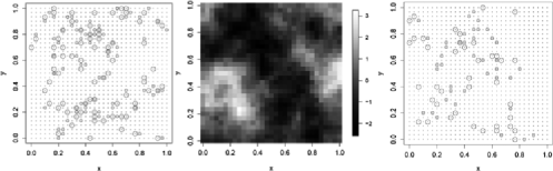
Figure 1: Example of an underlying reference field and two sampling schemes: the underlying reference field (middle) is a realization of a zero-mean isotropic Gaussian random field with a Matérn covariance function ($\nu=1$ and $\rho=0.2$). The other plots show two sampling schemes for $B^{\mathrm{true}}$ (big circles) and $A^{\mathrm{true}}$ (small circles): $n_{\mathrm{B}}=n_{\mathrm{A}}=80$ and $\kappa=1$ on the left-hand side and $n_{\mathrm{B}}=n_{\mathrm{A}}=40$ and $\kappa=4$ on the right-hand side. The dots correspond to the 961 possible point locations.

Let $A=\{A^{\mathrm{true}},A^{\mathrm{cont}}\}$ and $B=\{B^{\mathrm{true}},B^{\mathrm{cont}}\}$, where “true” denotes the part of each point set which stems from the underlying reference field $\tilde{\mathbf{z}}$ and “cont” denotes the contaminated part. The term “contaminated” refers to the points which do not follow the field model well and so will not be helpful in the alignment. Hence, the contaminated points should be masked in the matching algorithm.

We obtain $B^{\mathrm{true}}$ by randomly choosing $k^{\mathrm{true}}_{\mathrm{B}}$ entries $i_{1},\ldots,i_{k^{\mathrm{true}}_{\mathrm{B}}}$ from $\tilde{\mathbf{z}}$ and adding independent Gaussian noise with standard deviation $\sigma_{\varepsilon}$ to the corresponding marks. For $B^{\mathrm{cont}}$, $k^{\mathrm{cont}}_{\mathrm{B}}=k_{\mathrm{B}}-k^{\mathrm{true}}_{\mathrm{B}}$ locations on the grid are chosen at random and the corresponding marks are random values from a uniform distribution on $[-c,c]$. To obtain $A^{\mathrm{true}}$, we introduce a nearness parameter $\kappa\in\mathbb{N}$ and define a set of grid points $\mathcal{U}_{\kappa}$ as the union of neighborhoods around the points $\mathbf{x}^{\mathrm{B}}_{i}$ ($i=1,\ldots,k^{\mathrm{true}}_{\mathrm{B}}$), where each neighborhood contains the vertically, horizontally and diagonally adjacent grid points in a $(2\kappa+1)\times(2\kappa+1)$-box around the corresponding $\mathbf{x}^{\mathrm{B}}_{i}$. The parameter $\kappa$ therefore measures the nearness between points in terms of grid point locations rather than Euclidean distance which is further demonstrated in Figure 1. The point locations $\mathbf{x}^{\mathrm{A}}_{j}$ ($i=1,\ldots,k^{\mathrm{true}}_{\mathrm{A}}$) which belong to the matching part of $A$ are then chosen at random from $\mathcal{U}_{\kappa}$ and $A^{\mathrm{true}}$ is obtained by adding independent Gaussian noise with standard deviation $\sigma_{\varepsilon}$ to the corresponding marks $\tilde{z}(\mathbf{x}^{\mathrm{A}}_{j})$ ($i=1,\ldots,k^{\mathrm{true}}_{\mathrm{A}}$). Finally, the $k^{\mathrm{cont}}_{\mathrm{A}}=k_{\mathrm{A}}-k^{\mathrm{true}}_{\mathrm{A}}$ points in $A^{\mathrm{cont}}$ are obtained in the same way as the contamination points in $B$.

Note that this simulation scheme does not create pairwise correspondences between points in $A^{\mathrm{true}}$ and $B^{\mathrm{true}}$. Although we have used a nearness criterion in our simulation method, we have not estimated point correspondences in the course of the MCMC algorithm.

For our simulation study we consider three realizations of $\tilde{\mathbf{Z}}$, and for each of these realizations we define 12 different pairs of marked point sets by varying the parameters $k^{\mathrm{true}}=k^{\mathrm{true}}_{\mathrm{A}}=k^{\mathrm{true}}_{\mathrm{B}}\in\{40,80\}$, $k^{\mathrm{cont}}=k^{\mathrm{cont}}_{\mathrm{A}}=k^{\mathrm{cont}}_{\mathrm{B}}\in\{0.05k^{\mathrm{true}},0.1k^{\mathrm{true}},0.15k^{\mathrm{true}}\}$ and $\kappa\in\{1,4\}$. Moreover, we choose $c=7$ and $\sigma_{\varepsilon}=\sqrt{0.02}$. Generated as above, the 36 pairs $A$ and $B$ are recorded in the optimal relative position, and the optimal mask vectors are $\bolds\lambda_{\mathrm{A}}^{T}=(\mathbf{1}_{k^{\mathrm{true}}_{\mathrm{A}}}^{T},\mathbf{0}_{k^{\mathrm{cont}}_{\mathrm{A}}}^{T})$ and $\bolds\lambda_{\mathrm{B}}^{T}=(\mathbf{1}_{k^{\mathrm{true}}_{\mathrm{B}}}^{T},\mathbf{0}_{k^{\mathrm{cont}}_{\mathrm{B}}}^{T})$.

4.2 Hyperparameter settings

For each pairwise superposition 50,000MCMC iterations are carried out, and each iteration contains five blocks updating the rotation parameter (proposal standard deviation: $0.75^{\circ}$), the translation vector (proposal standard deviation: 0.01), the precision parameter and the two mask vectors, respectively. The Kernel Carbo similarity calculations are based on the exponential kernel, that is, (5) with $\nu=0.5$ (whereas $\nu=1$ was used for simulating the data). Initially we use $\rho=0.6$, but, within the first 1,000 iterations, this value is dynamically reduced to $\rho=0.2$. This initial phase allows the algorithm to home in on a good alignment even if the two points sets are far away from their optimal relative position. Moreover, we use $\beta=0.05$ and $\alpha=200$, and these values ensure a desirable interaction between the obtained dissimilarity values and the proposed precision values at each iteration. We include $\zeta$ as a variable parameter in our simulation study and consider $\zeta\in\{10,50,90\}$, and we fix $\zeta_{I}=1$.

To overcome the difficulty of getting trapped in local modes, we propose a big change of the rigid body parameters by using increased values for the standard deviations of the random walk proposals every 125 iterations. Moreover, we restart the algorithm if the Carbo distance exceeds 0.3 after 7,500 iterations.

4.3 Results

For each of the 108 (36 pairs of point sets $\times$ 3 values of $\zeta$) considered MCMC runs, the starting position of the movable point set $B$ is obtained by rotating and translating it from its original (simulated) position using $\bolds\Gamma(\theta_{0})$ and $\bolds\gamma_{0}$ where ${\theta_{0}}$ and ${\gamma_{0}}_{i}$ $(i=1,2)$ are uniformly distributed on $[-20^{\circ},20^{\circ}]^{3}$ and $[-0.1,0.1]$, respectively. Moreover, both mask vectors are initiated using $\lambda_{i}^{\mathrm{M}}\sim\operatorname{Bernoulli}(0.5)$ ($i=1,\ldots,k_{\mathrm{M}}$, $M\in\{A,B\}$). The performance of each run is then assessed in terms of the root mean square deviation (RMSD) between the original position of $B$ and its MAP position.

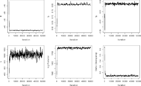
Figure 2: Top row: trace plot of the rigid-body parameters (in terms of the initial relative position of the two points sets under consideration). Bottom row: trace plots of the precision parameter, the log-posterior (up to a constant) and the Kriged Carbo distance. In all plots, every 100th simulated value is displayed.

Figures 2–4 show the typical output of a successful run. Figures 2 and 3 indicate that the algorithm converges quickly, and from Figure 2 it can be seen that there is an interplay between the precision parameter $\tau$ and the Kernel Carbo distance: until a good alignment is obtained, small distances lead to larger precision values which in turn yield small distances. Figure 3 shows the trace plots for the number of points which are involved in the field calculation and are hence considered to belong to $A^{\mathrm{true}}$ and $B^{\mathrm{true}}$, respectively, and a (post burn-in) summary of the two mask vectors is displayed in the bottom row of Figure 3. In this particular example, the optimal mask vectors are $\bolds\lambda_{\mathrm{M}}^{T}=(\mathbf{1}_{80}^{T},\mathbf{0}_{12}^{T})$ ($M=A,B$), and the algorithm is able to reconstruct the mask vector very well. Figure 4 shows that the MAP position of the movable point set is very similar to the original one.

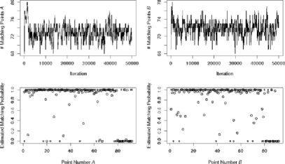
Figure 3: Top row: trace plots of the number of points involved in the kriging procedure. Bottom row: two possible point estimates for the mask vectors of $A$ (left) and $B$ (right). The big circles show the mean values of the $(0,1)$-entries for the masks vectors (which can be interpreted as the estimated probability for the corresponding landmark to belong to the common reference field), and the small circles display the observed mask vectors at the MAP iteration. The total number of points in $A$ and $B$ is 92, and the last 12 points in each set are contamination points.

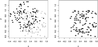
Figure 4: Successful alignment: the circles on the left-hand side show the initial position of point set $B$, and the circles on the right-hand side show the position of $B$ at the MAP iteration. The optimal position is displayed by the crosses on both sides. The algorithm is able to reduce the RMSD to the optimal position from 0.479 (left) to 0.032 (right).

We consider an alignment to be successful if $\operatorname{RMSD}\leq 0.1$. Table 1 shows the percentages of success for various parameter settings in the row “setting 1,” with an overall success rate of 76% out of the 108 MCMC runs. As expected, the largest number of true points in combination with the fewest number of contamination points gives the highest success rate (89%), whereas the smallest number of true points in combination with the highest number of contamination points gives the lowest success rate ($44\%$). In combination with these extreme cases, the impact of the nearness parameter is most striking with $22\%$ success for ($k^{\mathrm{true}}=40,k^{\mathrm{cont}}=6$, $\kappa=4)$ and $100\%$ for ($k^{\mathrm{true}}=80,k^{\mathrm{cont}}=4,\kappa=1)$. Overall, the impact of $\kappa$ can be summarized as $85\%$ success for $\kappa=1$ and $67\%$ success for $\kappa=4$. Interestingly, the success rate increases with $\zeta$.

Table 1: The percentages of MCMC runs which are regarded as a success (i.e., $\operatorname{RMSD}<0.1$) for different parameter settings. The column “all” shows the percentage of successes out of all 108 simulations for the corresponding setting

					$\bolds{k^{\mathrm{true}}=80}$	$\bolds{k^{\mathrm{true}}=40}$
	All	$\bolds{\zeta=10}$	$\bolds{\zeta=50}$	$\bolds{\zeta=90}$	$\bolds{k^{\mathrm{cont}}=4}$	$\bolds{k^{\mathrm{cont}}=6}$	$\bolds{\kappa=1}$	$\bolds{\kappa=4}$
Setting 1	76	61	81	86	89	44	85	67
Setting 2	48	33	47	61	83	17	52	44

The above results indicate that a satisfactory alignment can be obtained if the number of noncontamination points is large enough to represent the main features of the underlying reference field and large relative to the number of contamination points. Moreover, especially when the number of points is small and the sampling of the reference field is sparse, it is important that the noncontamination points in $A$ and $B$ represent the same features of the reference field (which is not always the case if $k^{\mathrm{true}}=40$ and $\kappa=4$). These trends can be emphasized by rerunning the experiments using $\theta\sim U_{[-60^{\circ},60^{\circ}]}$ and $\gamma_{i}\sim U_{[-0.3,0.3]}$ $(i=1,2)$ to obtain the starting position of $B$. For this more challenging setting (“setting 2”) the results are also provided in Table 1 with similar effects but lower success rates (48% overall).

In both settings, the performance of our alignment procedure can be improved if there are some points in $A$ and $B$ which can be identified as noncontamination points ab initio. For our examples, identifying some relevant points (on average 12 per point set) improves the overall success rate to 93% in the first setting and to 79% in the more challenging second setting. In many applications it may be possible to identify some relevant points so that the possibility of incorporating this knowledge is a valuable tool for improving the alignment.

Finally, we rerun the above experiments with different values for the range parameter $\rho$. For example, with $\rho=0.3$, overall success rates of 77% in the first and 48% in the second setting are achieved, and for $\rho=0.1$, the corresponding success rates are 77% and 52%. These results demonstrate that choosing the exact covariance function for the spatial interpolation is not crucial for the performance of the algorithm, although performance does deteriorate for much larger $\rho$. For example, a leave-one-out type method for identifying the contamination points combined with a pooled version of an experimental semivariogram [e.g., Wackernagel (2003), page 47] can be applied to estimate an approximate covariance function which has yielded satisfactory results in some further experiments.

4.4 Three-dimensional example

We now consider a small three-dimensional simulation study which mimics the molecule alignment problem of Section 5. As a starting point we take the positions of the first $25$ atoms of the first molecule in the steroid data set and generate the atom positions of a second “molecule” using a small perturbation (independent zero mean normal with standard deviation $0.01$). Then a zero mean isotropic Gaussian random field with Matérn covariance function $(\nu=0.5,\rho=5)$ is simulated at the combined set of the 50 points. To introduce contamination points, the last five points in each configuration have their coordinates and marks perturbed by independent $N(0,3^{2})$ errors. Finally, both molecules are centered and the molecules are uniformly rotated.

For various choices of the hyperparameters $\beta$ and $\zeta$ we run $100$ Monte Carlo simulations of the Bayesian alignment procedure. Each time the two marked point sets and their starting relative position are generated as above. The parameters $\nu=0.5$ and $\alpha=31$ are kept fixed and the range parameter is dynamically reduced from $\rho=20$ to $\rho=5$ during the matching procedure. Each simulation is restarted if the Kernel Carbo distance is greater than $0.1$ after $1\mbox{,}000$ iterations (up to a maximum of $30$ restarts). When the algorithm reaches $2\mbox{,}000$ iterations the final position and the MAP position of the movable molecule $B$ are recorded.

In this situation the success of the algorithm can be measured in terms of the first 20 atoms of $B$ by taking the corresponding $\operatorname{RMSD}$ between its MAP and its true position. The results of the simulation study are given in Table 2. As expected, the number of unmasked points in $B$ increases with $\zeta$. Interestingly, this consistently also leads to improved $\operatorname{RMSD}$ values—even in situations where a large value of $\zeta$ forces the algorithm to include more than the desired 20 points. In terms of the obtained Carbo distance, the impact of $\beta$ exceeds that of $\zeta$. This is also expected, as the mean of the full conditional distribution of the precision parameter $\tau$ (cf. Section 3.2) decreases with $\beta$ which in turn means that the algorithm is more prone to accept updates with larger Carbo distances.

Overall, this simulation study highlights that the Bayesian method works well in this controlled situation.

Table 2: Summary statistics from the posterior distribution in the simulation study. Columns 2–6 show the mean (and standard deviation) over 100 Monte Carlo simulations of the final number of unmasked points in molecule $A$ ($\sum\lambda^{\mathrm{A}}_{i}$); the final number of unmasked points in molecule $B$ ($\sum\lambda^{\mathrm{B}}_{j}$); the root mean square error ($\operatorname{RMSD}$); the number of new starts needed for the algorithm to be successful; and the Kriged Carbo distance at the final iteration. The last column shows the number of times out of $100$ simulations that the algorithm failed, that is, the Kernel Carbo distance was greater than $0.1$ after $1\mbox{,}000$ iterations for each of the maximum number of 30 restarts

$\bolds{(\beta,\zeta)}$	$\bolds{\sum\lambda^{\mathrm{A}}_{i}}$	$\bolds{\sum\lambda^{\mathrm{B}}_{j}}$	$\bolds{\operatorname{RMSD}}$	Starts	Carbo	Failures
$(0.0004,10)$	$18.41$	$17.42$	$0.1523$	$0.88$	$0.0204$	4
	$(2.39)$	$(2.13)$	$(0.5207)$	$(2.48)$	$(0.0226)$
$(0.0004,50)$	$21.16$	$20.00$	$0.0959$	$1.56$	$0.0178$	1
	$(1.45)$	$(0.97)$	$(0.6521)$	$(3.96)$	$(0.0195)$
$(0.0004,70)$	$21.66$	$20.43$	$0.0626$	$1.12$	$0.0263$	0
	$(1.53)$	$(0.97)$	$(1.1200)$	$(2.80)$	$(0.0208)$
$(0.004,10)$	$18.6$	$17.83$	$0.2193$	$0.67$	$0.0268$	0
	$(2.51)$	$(1.90)$	$(0.5492)$	$(1.21)$	$(0.026)$
$(0.004,50)$	$21.52$	$20.27$	$0.1018$	$1.55$	$0.0284$	1
	$(1.46$	$(1.08)$	$(0.4352)$	$(3.80)$	$(0.0560)$
$(0.004,70)$	$21.58$	$20.32$	$0.0605$	$1.19$	$0.0280$	0
	$(1.42)$	$(1.17)$	$(0.0734)$	$(3.34)$	$(0.0244)$
$(0.04,10)$	$20.90$	$19.47$	$0.1306$	$0.95$	$0.0342$	0
	$(1.75)$	$(1.60)$	$(0.5884)$	$(1.57)$	$(0.0187)$
$(0.04,50)$	$23.03$	$20.94$	$0.0739$	$1.59$	$0.0485$	1
	$(1.35)$	$(1.19)$	$(0.2748)$	$(3.75)$	$(0.0544)$
$(0.04,70)$	$23.15$	$20.92$	$0.0513$	$2.26$	$0.0472$	0
	$(1.37)$	$(1.04)$	$(0.0629)$	$(4.41)$	$(0.0258)$

5 Application to steroid molecules

The concept of molecular similarity is of great importance because similar molecules can be expected to exhibit a similar biochemical activity and hence drug potency. The data for the 31 steroids considered by Dryden, Hirst and Melville (2007) are given in the form of a set of unlabeled, marked points where the coordinates of the points correspond to the atom coordinates of each molecule, and the marks are the partial charge values and the van der Waals radii. The data set can be found in the supplementary materials [Czogiel, Dryden and Brignell (2011b)]. The Kernel Carbo index developed in this paper can therefore directly be utilized to assess the similarity between the steroids. Also, in particular, the assumption of a common underlying reference field seems suitable for this application because all molecules bind to the same receptor protein. The underlying reference field can therefore be interpreted as a negative imprint of the binding pocket of the receptor. The MCMC scheme described in Section 3 then determines the parts of each molecule which correspond to the reference field and aligns the molecules based on the similar parts only so that the resulting relative position should reproduce the relative binding positions of the steroids.

In order to investigate the possibility of multiple binding modes (and hence reference fields), we shall also consider an analysis of subgroups of the data. In particular, we consider the three activity classes.

5.1 Pairwise alignment

In our application we use the Gaussian kernel (6) for the spatial interpolation of both the partial charge values and the van der Waals radii. The range parameter $\rho$ for the electrostatic field is thereby estimated by visual inspection of a pooled empirical semivariogram function ($\rho_{Q}=6.35$), and the practical range of the steric (shape) field is taken to be the largest van der Waals radius in the data set ($\rho_{S}=1.7/\sqrt{3}=0.9815$).

In our simulation studies we dynamically reduced the range parameter to help the algorithm home in on a good solution. Here, we apply a different concept using a weighted average of the two univariate partial Carbo indices and choosing the weights dynamically as $w_{Q}=\frac{N_{I}-i}{N_{I}}$ and $w_{S}=\frac{i}{N_{I}},i=1,\ldots,N_{I}$, during an initial phase of $N_{I}=1\mbox{,}500$ iterations. This directly mimics real-life molecular recognition where the long-range electrostatic attraction governs the initial approach of the molecules, whereas the short-range repulsive steric forces gradually take over and become the chief manipulator for the binding affinity [e.g., Richards (1993)].

We use $\alpha=31$ and $\beta=0.04$, and the value for the penalty parameter is chosen as $\zeta=3$. As standard deviations of the proposal distributions we use $\eta_{1}=3.25^{\circ}$ for the rotation parameters and $\eta_{2}=0.25\mbox{ \AA}$ for the translation parameters, and these values ensure acceptance rates between 20% and 40%. The standard deviation for the rotation parameters is thereby in line with previously described proposal distributions for rotation parameters in the molecular context [e.g., Green and Mardia (2006)]. We define the initial relative position of two molecules by first aligning both molecules along their principal axes. We then translate and rotate the movable molecule using $\bolds\gamma_{0}$ and $\bolds\Gamma(\bolds\theta_{0})$, where ${\gamma_{0}}_{i}$ $(i=1,2,3)$ and ${\theta_{0}}_{i}$ $(i=1,2,3)$ are uniformly distributed on $[-5\mbox{ \AA},5\mbox{ \AA}]$ and $[-90^{\circ},90^{\circ}]$, respectively.

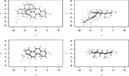
Figure 5: Two orthographic projections ($x$–$y$ and $x$–$z$ Cartesian planes) of the atoms in the starting position (top row) and the MAP position for the alignment (bottom row) of steroid molecules aldosterone and androstanediol. The carbon rings are indicated by lines for each molecule. The unit of all axes is Ångström (Å).

As our MCMC algorithm is asymmetric in the sense that the relative position of the molecules is changed by moving only one molecule whereas the position of the other one is fixed, we consider all $31\cdot 30=930$ pairwise superpositions. In the majority of cases, the algorithm converges quickly and the trace plots show a similar behavior as the ones in Figures 2 and 3. However, like in the simulation studies, the algorithm can sometimes get trapped in a local mode (which mostly corresponds to an alignment along the wrong principal axes in this application) so that a restart is necessary. Figure 5 shows an example result where the steroid aldosterone has successfully been superimposed onto androstanediol.

The specific choice of Gaussian kernel is not crucial to the success of the algorithm for the steroids data. Similar alignments of the steroids have been obtained using the Matérn kernel with $\nu=0.5,\nu=1,\nu=2$ for many examples, but it is important that the range parameter is well chosen. We found that with $\rho_{S}\approx 1$ the method worked well for any choice of covariance kernel we used, but if $\rho_{S}$ is too large (e.g., $\rho_{S}\approx 3$), then the alignment is cruder and the algorithm is more prone to failure for any choice of covariance function.

5.2 Prior sensitivity

To investigate the sensitivity of the analysis to the prior distributions, we again consider the alignment of the two molecules aldosterone and androstanediol. Table 3 shows how different values of the penalty parameter

Table 3: The impact of the penalty parameter (first four rows) and $\alpha$ (last four rows) on the marginal posterior distribution of the parameters of interest. The credibility intervals are based on every 20th value of the parameters recorded after the burn-in period

$\bolds{\zeta}$	95% CI for $\bolds{\tau}$	95% CI for $\bolds{\sum_{j}\lambda^{\mathrm{A}}_{j}}$	95% CI for $\bolds{\sum_{j}\lambda_{j}^{\mathrm{B}}}$
2	$(226.62,543.78)$	$(34,46)$	$(34,45)$
3	$(230.93,543.30)$	$(37,49)$	$(38,48)$
4	$(250.69,562.65)$	$(40,51)$	$(40,49)$
5	$(244.67,548.41)$	$(41,51)$	$(42,51)$
$\bolds{\alpha}$	95% CI for $\bolds{\tau}$	95% CI for $\bolds{\sum_{j}\lambda^{\mathrm{A}}_{j}}$	95% CI for $\bolds{\sum_{j}\lambda_{j}^{\mathrm{B}}}$
21	$(102.53,315.95)$	$(36,48)$	$(37,48)$
31	$(221.14,515.13)$	$(38,49)$	$(38,49)$
41	$(344.68,770.30)$	$(38,48)$	$(39,49)$
51	$(432.36,1010.77)$	$(35,48)$	$(37,50)$

$\zeta$ affect the empirical (post burn-in) 95% credibility intervals for the number of included atoms for both molecules based on 10,000 iterations. As expected, the total number of included atoms increases with $\zeta$. As the two molecules in the example run are structurally very similar, they can be aligned more closely if more atoms are included so that the credibility interval for the precision parameter is shifted toward higher values as $\zeta$ increases. After a certain threshold, however, even larger values for the penalty parameter force the algorithm to include more atoms in the similarity calculations than desired and the precision decreases. Moreover, Table 3 shows that—in terms of the number of included atoms—the algorithm is robust against changes of $\alpha$. Also, as the posterior mean and variance of the precision parameter directly depend on $\alpha$, the credibility intervals for $\tau$ become wider and get shifted toward higher values as $\alpha$ increases.

5.3 Chemical relevance

The pairwise distances which result from the 930 superpositions can be regarded as chemically meaningful if they reflect the membership of the steroid molecules to the three activity classes, that is, if steroids within an activity class can be aligned more closely than those from different activity classes. In terms of our assumption about a common underlying reference field, such a result would indicate that there are actually three different reference fields which exhibit different small scale variations and hence different abilities to fit in to the protein binding pocket.

We assess the chemical relevance of our results by performing two cluster analyses using Ward’s (1963) method. To account for the asymmetry in our alignment method, the applied pairwise dissimilarity measures for two molecules $A$ and $B$ are thereby based on both the MCMC run which superimposes $A$ on $B$ and the MCMC run which superimposes $B$ on $A$. In particular, we use $D_{\mathrm{mean}}(A,B)=\sqrt{\hat{D}^{\mathrm{mean}}_{A\rightarrow B}\hat{D}^{\mathrm{mean}}_{B\rightarrow A}}$ and $D_{\mathrm{MAP}}(A,B)=\sqrt{\hat{D}^{\mathrm{MAP}}_{A\rightarrow B}\hat{D}^{\mathrm{MAP}}_{B\rightarrow A}}$, where the arrow denotes the direction of the superposition, and “mean” and “MAP” indicate which type of (post burn-in) point estimate for the parameters is inserted into the Carbo dissimilarity measure (11).

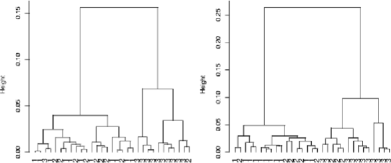
Figure 6: Cluster analysis using Ward’s method: the left-hand side dendrogram is based on $D_{\mathrm{mean}}(\cdot)$, and the dendrogram on the right-hand side is calculated using $D_{\mathrm{MAP}}(\cdot)$. The labels correspond to the activity classes of the steroids (1${}={}$high, 2${}={}$intermediate, 3${}={}$low).

Figure 6 shows the dendrograms resulting from the cluster analyses. It is notable that both distance measures lead to a very good separation of high and low activity steroids. In particular, the cluster analysis based on $D_{\mathrm{MAP}}(\cdot)$ is at the highest level able to separate these two activity classes completely. Overall, our distance can separate the activity classes as well as the distance which Dryden, Hirst and Melville (2007) found to have the highest separation power, and it clearly outperforms the other distances defined in their paper.

The dendrograms indicate that it is plausible to assume that there are at least two different reference fields underlying the steric properties of the steroids. It is therefore of interest to determine these fields and examine where differences occur, as they could give rise to the different binding activities. In the following we will do so in a two-step procedure where our field GPA approach is first applied to all 31 steroids to obtain the overall optimal relative position of the molecules and then to the subgroups as defined by the activity classes which will provide the appropriate masks.

5.4 Overall multiple alignment

When carrying out the overall optimal alignment of all 31 steroid molecules, the pairwise superpositions in step 1 of Algorithm 1 are performed as described before but with $\zeta=2$ to incorporate the knowledge that the reference molecule in all superpositions has a small number of atoms. The superpositions on the mean fields (step 7) are obtained using only the dissimilarities of the steric fields. As the initial molecular fields obtained in step 1 are good approximations of the fields which minimize the multiple Kernel Carbo index, we use $\alpha=600$ and $\beta=0.0001$ to ensure that the full conditional distribution of the precision parameter has a large mean value at each iteration, and we reduce the standard deviations of the proposal distributions for the rigid body parameters to $\eta_{1}=0.75$ Å and $\eta_{2}=0.03^{\circ}$. Moreover, we set the number of iterations for each MCMC run in step 7 to 500, and the tolerance value to $\mathrm{tol}=0.0001$. The algorithm is therefore used as a stochastic optimizer.

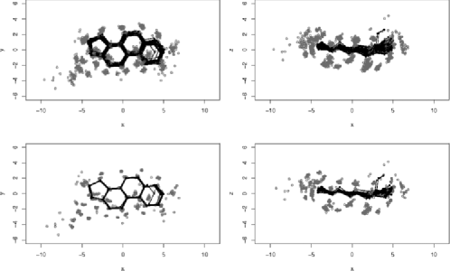
Figure 7: Top row: orthographic projections of the relative position of the 31 steroid molecules that results from step 1 of Algorithm 1. Bottom row: orthographic projections of the final relative position. The random starting positions of the molecules are not displayed.

The algorithm converges after the fourth field GPA iteration. Figure 7 shows orthographic views of the resulting overlays, that is, projections of the three-dimensional data into the $x$–$y$ and $x$–$z$ Cartesian planes. The superposition after step 1 of the field GPA algorithm is displayed in the top row, and the bottom row shows the final overlay. For clarity, the random starting positions of the steroids are not displayed in this picture.

5.5 Alignment within activity class subgroups

We now carry out the field GPA algorithm in subgroups of the data to allow for the possibility of different underlying multiple fields. Specifically, we consider the three activity classes of high, medium and low binding affinity to the receptor. The estimated mask vectors from each underlying field are then used together with the relative position of all molecules obtained in the overall field GPA to calculate mean fields for each group.

Figure 8 displays different cross sections of the mean field for each activity class. Light points thereby correspond to locations where the displayed steric field takes a large value, whereas dark points show field values close to zero.

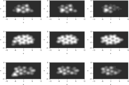
Figure 8: Cross sections of the mean steric fields of the three activity groups (left column: high activity, middle column: medium activity, right column: low activity). The different rows display cross sections at $z=-1.5$ (top row), $z=0$ (medium row) and $z=1.5$ (bottom row). Light points correspond to locations with large value of the displayed field, whereas dark values show points with values close to zero.

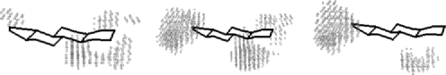
Figure 9: Thresholded $t$-fields resulting from pairwise comparisons of the steric mean fields of the three activity classes. Left-hand side: low vs. medium activity class, middle: low vs. high activity class, right-hand side: medium vs. high activity class. The shaded areas display regions where the $t$-field takes absolute values of larger than eight.

As expected, the observed differences are most pronounced between the mean fields of the high and the low activity group. To assess the differences for each pair ($C_{a},C_{b}$) of activity classes ($a,b=1,2,3;a\neq b$) numerically, we consider a (two sample) $t$-field of the form

$$t_{ab}(\mathbf{x})=\frac{\bar{Z}_{a}(\mathbf{x})-\bar{Z}_{b}(\mathbf{x})}{s^{*}_{\mathrm{pool}}(\mathbf{x})\sqrt{{1/n_{a}}+{1/n_{b}}}},\qquad\mathbf{x}\in\mathbb{R}^{3},$$ (13)

where $n_{a}$ and $n_{b}$ denote the number of molecules in activity class $C_{a}$ and $C_{b}$, respectively, $\bar{Z}_{a}(\mathbf{x})$ and $\bar{Z}_{b}(\mathbf{x})$ denote the corresponding mean fields, and $s^{*2}_{\mathrm{pool}}(\mathbf{x})=s^{2}_{\mathrm{pool}}(\mathbf{x})+d$ is the pooled variance (with $d=0.001$ a small offset to avoid spuriously large values in regions far away from the center). For each pairwise comparison we define a three-dimensional grid $G$ and calculate a $t$-value of the form (13) at a large number of points ($142\mbox{,}598$ here). Here we use (13) as an exploratory tool to see where the most pronounced differences occur. Figure 9 shows the regions in which the (absolute) $t$-field for each comparison exceeds a threshold of $8$. A formal test which takes into account the multiple comparison problem and the spatial smoothness of the $t$-field could be applied using a threshold based on the excursion sets of Gaussian fields [e.g., Worsley (1994), Taylor and Worsley (2008)], which has been extensively used in fMRI studies.

From both Figures 8 and 9 it can be seen that the main feature which distinguishes the high activity class from the other two classes is that the very active molecules commonly extend to the left of the ring structure much more than the other molecules, where by ring structure we mean the carbon rings as shown in Figure 5. From the original data we can get the additional information that the associated atoms are oxygen and carbon atoms. Another interesting difference is located at the top right-hand side of the molecules where the low activity class differs from the other two classes in the location of oxygen atoms. These findings are in line with Figure 9 in Dryden, Hirst and Melville (2007) and support the conjecture that the steric properties of the steroid molecules have a discriminating effect with respect to the binding affinity toward the CBG receptor.

6 Discussion

Our methodology for aligning and comparing unlabeled marked point sets is based on spatial interpolation of the given marks and hence on a continuous representation of shape. The major advantages of our approach are that point correspondences do not need to be estimated and that the incorporated mask vectors automatically determine the similar regions of the considered point sets while ignoring the rest, which helps to reduce the level of noise in the alignment procedure.

Our approach is related to a number of previously proposed methods. For example, it provides a probabilistic framework and generalization of the SEAL algorithm [Kearsley and Smith (1990)] which is well established in the field of rational drug design and essentially uses the $L_{2}$-Carbo index together with a Gaussian covariance function. Our multiple alignment approach is related to the Bayesian model proposed by Dryden, Hirst and Melville (2007) which uses a similar concept but formulated only in terms of the point locations. Contrary to that, a hidden point configuration in the fully model-based Bayesian approach by Ruffieux and Green (2009) is integrated out and the multiple alignment of $n$ point sets involves all $2^{n}-n-1$ possible types of matches. The fact that our field-based approach naturally incorporates the additional information given by the marks is an additional difference to the previous approaches which is of particular advantage in the multiple alignment setting, as the resulting mean fields allow straightforward post-processing.

In this paper we obtain the similarity index at the maximum a posteriori (MAP) estimates of the rigid-body transformations and mask parameters because this gives an approximation to the Kernel Carbo index (4). We could alternatively consider a full posterior analysis and work with the posterior distribution. A similar issue occurs in Bayesian shape analysis of unlabeled landmark configurations [Green and Mardia (2006), Dryden, Hirst and Melville (2007), Schmidler (2007)] where either a marginal approach (integrating out nuisance parameters) or a conditional approach (conditioning at the MAP) could be used. We compared the two approaches for unlabeled landmarks in other work [Kenobi and Dryden (2010)] and the overall performance was similar in the situations considered. This can be explained by the similarity of the marginal and conditional posteriors when a Laplace approximation is accurate (e.g., highly concentrated posterior distributions for the nuisance parameters).

Finally, as molecules are fuzzy bodies of electronic clouds rather than discrete sets of atoms, our approach is particularly suited for the described application. However, as it does not require any predefined point-by-point correspondence, it could be an approach to resolve the alignment problem for a fairly broad range of applications. Examples include matching organs in medical images, matching objects in images of real-world scenes (e.g., faces) in photographs or clouds in satellite images.

References

- Aronszajn (1950) {barticle}[mr] \bauthor\bsnmAronszajn, \bfnmN.\binitsN. (\byear1950). \btitleTheory of reproducing kernels. \bjournalTrans. Amer. Math. Soc. \bvolume68 \bpages337–404. \bidissn=0002-9947, mr=0051437 \endbibitem
- Carbo, Leyda and Arnau (1980) {barticle}[auto:STB—2011-03-03—12:04:44] \bauthor\bsnmCarbo, \bfnmR.\binitsR., \bauthor\bsnmLeyda, \bfnmL.\binitsL. and \bauthor\bsnmArnau, \bfnmM.\binitsM. (\byear1980). \btitleAn electron density measure of the similarity between two compounds. \bjournalInternational Journal of Quantum Chemistry \bvolume17 \bpages1185–1189. \endbibitem
- Cressie (1993) {bbook}[mr] \bauthor\bsnmCressie, \bfnmNoel A. C.\binitsN. A. C. (\byear1993). \btitleStatistics for Spatial Data. \bpublisherWiley, \baddressNew York. \bidmr=1239641 \endbibitem
- Czogiel, Dryden and Brignell (2011a) {bmisc}[auto:STB—2011-03-03—12:04:44] \bauthor\bsnmCzogiel, \bfnmI.\binitsI., \bauthor\bsnmDryden, \bfnmI. L.\binitsI. L. and \bauthor\bsnmBrignell, \bfnmC. J.\binitsC. J. (\byear2011a). \bhowpublishedSupplement to “Bayesian matching of unlabeled marked point sets using random fields, with an application to molecular alignment.” DOI:10.1214/11-AOAS486SUPPA. \endbibitem
- Czogiel, Dryden and Brignell (2011b) {bmisc}[auto:STB—2011-03-03—12:04:44] \bauthor\bsnmCzogiel, \bfnmI.\binitsI., \bauthor\bsnmDryden, \bfnmI. L.\binitsI. L. and \bauthor\bsnmBrignell, \bfnmC. J.\binitsC. J. (\byear2011b). \bhowpublishedSupplement to “Bayesian matching of unlabeled marked point sets using random fields, with an application to molecular alignment.” DOI:10.1214/11-AOAS486SUPPB. \endbibitem
- Dryden, Hirst and Melville (2007) {barticle}[mr] \bauthor\bsnmDryden, \bfnmIan L.\binitsI. L., \bauthor\bsnmHirst, \bfnmJonathan D.\binitsJ. D. and \bauthor\bsnmMelville, \bfnmJames L.\binitsJ. L. (\byear2007). \btitleStatistical analysis of unlabeled point sets: Comparing molecules in chemoinformatics. \bjournalBiometrics \bvolume63 \bpages237–251. \biddoi=10.1111/j.1541-0420.2006.00622.x, issn=0006-341X, mr=2345594 \endbibitem
- Dryden and Mardia (1998) {bbook}[mr] \bauthor\bsnmDryden, \bfnmI. L.\binitsI. L. and \bauthor\bsnmMardia, \bfnmK. V.\binitsK. V. (\byear1998). \btitleStatistical Shape Analysis. \bpublisherWiley, \baddressChichester. \bidmr=1646114 \endbibitem
- Good, So and Richards (1993) {barticle}[pbm] \bauthor\bsnmGood, \bfnmA. C.\binitsA. C., \bauthor\bsnmSo, \bfnmS. S.\binitsS. S. and \bauthor\bsnmRichards, \bfnmW. G.\binitsW. G. (\byear1993). \btitleStructure-activity relationships from molecular similarity matrices. \bjournalJ. Med. Chem. \bvolume36 \bpages433–438. \bidissn=0022-2623, pmid=8474098 \endbibitem
- Green and Mardia (2006) {barticle}[mr] \bauthor\bsnmGreen, \bfnmPeter J.\binitsP. J. and \bauthor\bsnmMardia, \bfnmKanti V.\binitsK. V. (\byear2006). \btitleBayesian alignment using hierarchical models, with applications in protein bioinformatics. \bjournalBiometrika \bvolume93 \bpages235–254. \biddoi=10.1093/biomet/93.2.235, issn=0006-3444, mr=2278080 \endbibitem
- Handcock and Wallis (1994) {barticle}[mr] \bauthor\bsnmHandcock, \bfnmMark S.\binitsM. S. and \bauthor\bsnmWallis, \bfnmJames R.\binitsJ. R. (\byear1994). \btitleAn approach to statistical spatial-temporal modeling of meteorological fields. \bjournalJ. Amer. Statist. Assoc. \bvolume89 \bpages368–390. \bidissn=0162-1459, mr=1294070 \bptnotecheck related \endbibitem
- Kearsley and Smith (1990) {barticle}[auto:STB—2011-03-03—12:04:44] \bauthor\bsnmKearsley, \bfnmS. K.\binitsS. K. and \bauthor\bsnmSmith, \bfnmG. M.\binitsG. M. (\byear1990). \btitleAn alternative method for the alignment of molecular structures: Maximizing electrostatic and steric overlaps. \bjournalTetrahedron Computer Methodology \bvolume3 \bpages315–633. \endbibitem
- Kenobi and Dryden (2010) {bmisc}[auto:STB—2011-03-03—12:04:44] \bauthor\bsnmKenobi, \bfnmK.\binitsK. and \bauthor\bsnmDryden, \bfnmI. L.\binitsI. L. (\byear2010). \bhowpublishedBayesian matching of unlabelled point sets using Procrustes and configuration models. Technical report, Univ. Nottingham. Available at arXiv:1009.3072v1. \endbibitem
- Kirkpatrick, Gelatt and Vecchi (1983) {barticle}[mr] \bauthor\bsnmKirkpatrick, \bfnmS.\binitsS., \bauthor\bsnmGelatt, \bfnmC. D.\binitsC. D. Jr. and \bauthor\bsnmVecchi, \bfnmM. P.\binitsM. P. (\byear1983). \btitleOptimization by simulated annealing. \bjournalScience \bvolume220 \bpages671–680. \bidissn=0036-8075, mr=0702485 \endbibitem
- R Development Core Team (2011) {bbook}[auto:STB—2011-03-03—12:04:44] \bauthor\bsnmR Development Core Team (\byear2011). \btitleR: A Language and Environment for Statistical Computing. \bpublisherR Foundation for Statistical Computing, \baddressVienna, Austria. \endbibitem
- Richards (1993) {barticle}[auto:STB—2011-03-03—12:04:44] \bauthor\bsnmRichards, \bfnmW. G.\binitsW. G. (\byear1993). \btitleComputers in drug design. \bjournalPure and Applied Chemistry \bvolume65 \bpages231–234. \endbibitem
- Ruffieux and Green (2009) {barticle}[mr] \bauthor\bsnmRuffieux, \bfnmYann\binitsY. and \bauthor\bsnmGreen, \bfnmPeter J.\binitsP. J. (\byear2009). \btitleAlignment of multiple configurations using hierarchical models. \bjournalJ. Comput. Graph. Statist. \bvolume18 \bpages756–773. \biddoi=10.1198/jcgs.2009.07048, issn=1061-8600, mr=2572636 \endbibitem
- Schmidler (2007) {bincollection}[mr] \bauthor\bsnmSchmidler, \bfnmScott C.\binitsS. C. (\byear2007). \btitleFast Bayesian shape matching using geometric algorithms. In \bbooktitleBayesian Statistics 8 \bpages471–490. \bpublisherOxford Univ. Press, \baddressOxford. \bidmr=2433204 \bptnotecheck related \endbibitem
- Stein (1999) {bbook}[mr] \bauthor\bsnmStein, \bfnmMichael L.\binitsM. L. (\byear1999). \btitleInterpolation of Spatial Data: Some Theory for Kriging. \bpublisherSpringer, \baddressNew York. \bidmr=1697409 \endbibitem
- Taylor and Worsley (2008) {barticle}[mr] \bauthor\bsnmTaylor, \bfnmJ. E.\binitsJ. E. and \bauthor\bsnmWorsley, \bfnmK. J.\binitsK. J. (\byear2008). \btitleRandom fields of multivariate test statistics, with applications to shape analysis. \bjournalAnn. Statist. \bvolume36 \bpages1–27. \biddoi=10.1214/009053607000000406, issn=0090-5364, mr=2387962 \endbibitem
- Wackernagel (2003) {bbook}[auto:STB—2011-03-03—12:04:44] \bauthor\bsnmWackernagel, \bfnmH.\binitsH. (\byear2003). \btitleMultivariate Geostatistics, \bedition3rd ed. \bpublisherSpringer, \baddressBerlin. \endbibitem
- Ward (1963) {barticle}[mr] \bauthor\bsnmWard, \bfnmJoe H.\binitsJ. H. Jr. (\byear1963). \btitleHierarchical grouping to optimize an objective function. \bjournalJ. Amer. Statist. Assoc. \bvolume58 \bpages236–244. \bidissn=0162-1459, mr=0148188 \endbibitem
- Worsley (1994) {barticle}[mr] \bauthor\bsnmWorsley, \bfnmK. J.\binitsK. J. (\byear1994). \btitleLocal maxima and the expected Euler characteristic of excursion sets of , and fields. \bjournalAdv. in Appl. Probab. \bvolume26 \bpages13–42. \biddoi=10.2307/1427576, issn=0001-8678, mr=1260300 \endbibitem