The CUSUM test for detecting structural changes in strong mixing processes

The CUSUM test for detecting structural changes in strong mixing processes

Abstract

Strong mixing property holds for a broad class of linear and nonlinear time series models such as ARMA and GARCH models. In this article we study correlation structure of strong mixing sequences, and some asymptotic properties are presented. We also present a new method for detecting change point in correlation structure of strong mixing sequences, and present a nonparametric CUSUM test statistic for this. Asymptotic consistency of this test statistics is shown. This method is applied to simulated data of some linear and nonlinear models and power of the test is evaluated. For linear models, it is shown that this method have a better performance in compare to Berkes et al.(2009).

MSC: Primary 62M10, 60F17, Secondary 62G20, 62G10.
Key words and Phrases: structural changes, Strong mixing, Functional central limit theorem, CUSUM test, Brownian bridge.

1 Introduction

Change point detection in a sequence of random variables was first proposed by Page(1954). This study started by detecting changes in the mean of a sequence of independent random variables and then extended to dependent sequences. Change point detection is widely used in various fields such as quality control, economics, finance and medicine. Review of earlier works can be found in Csörgö and Horváth(1988), Brodsky and Darkhovsky (1993) and Csörgö and Horváth(1997).

Among different methods for change point detection, the CUSUM test proposed by Page(1954), for mean change detection, is widely used for its simplicity. Inclán and Tiao(1994) proposed a CUSUM of squares test for testing a variance change in i.i.d. normal random variables. Lee and Park(2001) extended the CUSUM test of squares test of Inclán and Tiao(1994) for linear processes. Lee et al.(2003) studied change of parameters in a random coefficient AR(1) model, thus detecting changes in the auto-covariances of a linear process Galeano and Pena(2007) studied changes in variance and correlation structure of the multivariate time series. Zhou and Liu(2009) used a weighted CUSUM statistic for mean change detection in infinite variance AR(p) process. Berkes et al.(2009) considered a CUSUM test to detect changes in the mean and in the covariance structure of a linear process. Recently Qin et al.(2010) studied mean change detection in $\alpha$-mixing processes.

In this article we study change in the correlation structure of strong mixing sequences. Let $\{X_{t}:t\geq 1\}$ be a stationary process. As a measure of dependence we use Rosenblatt’s $\alpha$-mixing coefficient as

$$\alpha_{X}(n,j)=\sup_{A,B}|P(A\cap B)-P(A)P(B)|,$$

where A and B are in the $\sigma$-fields ${\mathbf{M}}_{-\infty}^{n}(X)=\sigma\{X_{t};t<n\}$ and ${\mathbf{M}}_{n+j}^{\infty}(X)=\sigma\{X_{t};t>n+j\}$ respectively. The sequence $\{X_{t}\}$ is said to be $\alpha$-mixing or strong mixing (SM) if

$$\alpha_{X}(j)=\sup_{n}\alpha_{X}(n,j)\rightarrow 0\ \ as\ j\rightarrow\infty.$$

Strong mixing processes are asymptotically independent. Strong mixing property holds for a large class of linear and nonlinear stationary time series such as ARMA and GARCH models, m-dependent processes, broad class of Gaussian processes and ergodic Markov processes( Bosq 1996, and Bradley 2005).

Ibragimov(1962) showed some results for stationary strong mixing sequences and proved central limit theorem for strict stationary SM processes. Davydov(1968) obtained some moment inequalities and Rio(1993) presented some covariance inequalities and bounds on the variance of partial sums of SM processes. Herrndorf(1985), Doukhan et al.(1994), and Merlevede and Peligard(2000) studied functional central limit theorem on SM processes. Romano and Thombs(1996) used central limit theorem, established by Ibragimov(1962), to show that sample auto-covariances of strictly stationary SM sequences converge in distribution to normal distribution.

By using functional central limit theorem for SM sequences, we propose a new test statistic for detecting changes in correlation structure of stationary strong mixing processes. This test is a nonparametric one and does not depend on any assumptions about the underlying distribution or model. The rest of this paper is organized as follows: In section 2 a nonparametric test statistic for detection of change points, in broad class of linear and non linear process, is constructed and its asymptotic properties, under no change null hypothesis, are studied. Also the consistency of this test statistic is shown in section 2. Section 3 is devoted to the simulation results on different linear and nonlinear models. In this section the method of Berkes et al.(2009) has been compared with the method of this paper for some some linear models. By simulation we show that this test statistic have a better performance and is more powerful in many cases.

2 Main results

In this section we present some preliminary results which will be used later in this paper. We present functional central limit theorem for sample auto-covariances of SM processes. We also introduce a new test statistic for detecting changes in the correlation structure of stationary SM processes, which we call CUSUM strong mixing(CSSM). Finally we show consistency and asymptotic convergence of this empirical CSSM test statistic.

Let $\{X_{n}\}$ be a sequence of random variables on some probability space $(\Omega,\mathcal{F},P)$, satisfying

$$E(X_{n})=0,\ \ \ E(X_{n}^{2})<\infty\ \ \ \ \mbox{for}\ \ n>0.$$

Let $S_{n}=X_{1}+...+X_{n}$ for $n>0$. Consider the Skorokhod space $D\equiv D[0,1]$ of all functions on $[0,1]$ which are right continuous with left limit. Let $W_{n}(t):\Omega\rightarrow D$ to be a random function as

$$W_{n}(t)=\frac{S_{[nt]}}{\sigma\sqrt{n}}\ \ \ \ \mbox{for}\ \ t\in[0,1],\ n>0.$$

If $W_{n}(t)$ is weakly convergent to a standard Brownian motion $W(t)$, then $X_{n}$ is said to satisfy the functional central limit theorem or strong invariance principle (Billingsley, 1999). Herrndorf(1985) proved functional central limit theorem for strong mixing sequences without stationarity assumption but assumed convergence of the variance of partial sums.

For $X_{1},X_{2},...$ as a sequence of zero-mean stationary process the sample auto-covariances $\hat{\gamma}_{n}(h)$, $h=0,...,n$, are defined as:

$$\hat{\gamma}_{n}(h)=\hat{\gamma}_{n}(-h)=\frac{1}{n}\sum_{i=1}^{n-h}X_{i}X_{i+h}.$$

Asymptotic covariance of sample autocovariances is known as Bartlett’s estimator and is defined as:

$$c_{hk}=\lim_{n\rightarrow\infty}nCov(\hat{\gamma}_{n}(h),\hat{\gamma}_{n}(k)).$$

Let

$$g^{*}_{n}(t):=\frac{[nt]}{\sqrt{n}}C^{-1/2}(\hat{\gamma}_{[nt]}(0)-\hat{\gamma}_{n}(0),\,\hat{\gamma}_{[nt]}(1)-\hat{\gamma}_{n}(1),...,\,\hat{\gamma}_{[nt]}(L)-\hat{\gamma}_{n}(L))^{T},$$

where $C=[c_{hk}]_{h,k=1}^{L+1}$ is the covariance matrix whose entries are defined by (2.3). Now we have the following result.
Theorem 1: Let $\{X_{n}\}_{n=1}^{\infty}$ be a stationary strong mixing process which satisfies:

• i) $\sup_{i}E|X_{i}|^{4+2\delta}<\infty$

• ii) $\sum_{k=1}^{\infty}\alpha_{X}(k)^{\delta/(2+\delta)}<\infty$ , for some $\delta\in(0,\infty)$

in which $\alpha_{X}(.)$ is the mixing coefficient, defined by (1.2). Then

$$g^{*}_{n}(t)^{T}.g^{*}_{n}(t)\Rightarrow\sum_{j=0}^{L}(W^{0}_{j}(t))^{2}\ \ \ \ \mbox{as}\ n\rightarrow\infty,$$

where $\Rightarrow$ denotes convergence in distribution, $W^{0}_{j}(.)$ are independent Brownian bridge, for $0\leq j\leq L$.

Before proceeding to the proof of this theorem we present some lemmas, which are necessary for our proof.

Lemma 1: (Davydov, 1968) Let the process $\{X_{t}\}$ be strong mixing, and random variables $\xi$ and $\eta$ be measurable with respect to ${\mathbf{M}}_{-\infty}^{n}(X)$ and ${\mathbf{M}}_{n+j}^{\infty}(X)$, introduced by (1.1), respectively. Moreover if the moments $E|\xi|^{p}$ and $E|\eta|^{q}$ exist for $p,q>0$ where $\frac{1}{p}+\frac{1}{q}<1$, then

$$|E\xi\eta-E\xi E\eta|\leq C[E|\xi|^{p}]^{1/p}[E|\eta|^{q}]^{1/q}[\alpha(n)]^{1-1/p-1/q}.$$

Lemma 2: Let $\{X_{n}\}_{n=1}^{\infty}$ be a zero-mean strong mixing process, where

$$\sum_{k=1}^{\infty}\alpha_{X}(k)^{\delta/(2+\delta)}<\infty,\ \ \mbox{and}\ \ \sup_{i}E|X_{i}|^{2+\delta}=M<\infty,\ \ \mbox{for some}\ \delta\in(0,\infty).$$

Then $\frac{E(S_{n})^{2}}{n}$ is convergent.

Proof of Lemma 2: By lemma 1,

$$E(S_{n})^{2}=\sum_{t=1}^{n}\sum_{s=1}^{n}E(X_{t}X_{s})\leq\sum_{t=1}^{n}\sum_{s=1}^{n}[E|X_{t}|^{p}]^{1/p}[E|X_{s}|^{q}]^{1/q}[\alpha_{X}(s-t)]^{1-1/p-1/q}.$$

Let $p=q=2+\delta$, then

$$\frac{1}{n}E(S_{n})^{2}\leq\frac{1}{n}M^{\frac{2}{2+\delta}}\sum_{i=-n}^{n}n[\alpha_{X}(i)]^{\delta/2+\delta}\leq M\sum_{i=-\infty}^{\infty}[\alpha_{X}(i)]^{\delta/2+\delta}\leq\infty.$$

An alternative proof for lemma 2 can be found in Rio (1993).

Proof of Theorem 1: Let

$$g_{n}(t):=\frac{[nt]}{\sqrt{n}}C^{-1/2}(\hat{\gamma}_{[nt]}(0)-{\gamma}(0),\hat{\gamma}_{[nt]}(1)-{\gamma}(1),...,\hat{\gamma}_{[nt]}(L)-{\gamma}(L))^{T},$$

where $\gamma(.)$ is auto-covariance function of $\{X_{t}\}$. By (2.4) and (2.6), it is immediate that

$$g^{*}_{n}(t)=g_{n}(t)-\frac{[nt]}{n}g_{n}(1).$$

Any Brownian bridge $W^{0}(t)$ has the same distribution as $W(t)-tW(1)$, where $W(t)$ is a standard Brownian motion (Billingsley, 1999).
Therefore if $g_{n}(t)\Rightarrow(W_{0}(t),W_{1}(t),...,W_{L}(t))^{T}$, where $W_{i}(t)$ are independent Brownian motions for $0\leq i\leq L$, then $g^{*}_{n}(t)\Rightarrow(W^{0}_{0}(t),W^{0}_{1}(t),...,W^{0}_{L}(t))^{T}$. So it is enough to show that $g_{n}(t)$ converges to a vector of Brownian motions.
As

$$g_{n}(t)=\frac{[nt]}{\sqrt{n}}C^{-1/2}\left(\begin{array}[]{c}\hat{\gamma}_{[nt]}(0)-\gamma(0)\\ \vdots\\ \hat{\gamma}_{[nt]}(L)-\gamma(L)\\ \end{array}\right)=\frac{C^{-1/2}}{\sqrt{n}}\left(\begin{array}[]{c}\sum_{i=1}^{[nt]}X_{i}X_{i}-[nt]\gamma(0)\\ \vdots\\ \sum_{i=1}^{[nt]-L}X_{i}X_{i+L}-[nt]\gamma(L)\\ \end{array}\right),$$

so by assuming

$$Y_{m,t}=X_{t}X_{t+m}-\gamma(m),\ \ \ \mbox{for}\ \ 0\leq m\leq L$$

we have that

$$g_{n}(t)=\frac{C^{-1/2}}{\sqrt{n}}\left(\begin{array}[]{c}\sum_{i=1}^{[nt]}Y_{m,i}\\ \vdots\\ \sum_{i=1}^{[nt]-L}Y_{m,i}\\ \end{array}\right)+\frac{C^{-1/2}}{\sqrt{n}}\left(\begin{array}[]{c}0\\ \gamma(1)\\ 2\gamma(2)\\ \vdots\\ L\gamma(L)\\ \end{array}\right).$$

By (2.7),

$${\mathbf{M}}_{-\infty}^{n}(Y)=\sigma\{Y_{m,t};t<n\}=\sigma\{X_{t}X_{t+m};t<n\}\subseteq{\mathbf{M}}_{-\infty}^{n+m}(X),$$

and

$${\mathbf{M}}_{n+j}^{\infty}(Y)=\sigma\{Y_{m,t};t>n+j\}=\sigma\{X_{t}X_{t+m};t>n+j\}\subseteq{\mathbf{M}}_{n+j}^{\infty}(X).$$

So relation (1.1) implies that, $\alpha_{Y_{m}}(j)\leq\alpha_{X}(j-m)$. Hence $\{Y_{m,t}\}$ form a zero mean, strong mixing process, where by assumption (ii),

$$\sum_{k=1}^{\infty}\alpha_{Y_{m}}(k)^{\delta/(2+\delta)}<\infty.\ \$$

Also by (2.7) and assumption (i),

$$\sup_{i}E|Y_{m,i}|^{2+\delta}<\infty,\ \$$

for some $\delta\in(0,\infty)$. Let $S_{m,n}=Y_{m,1}+...+Y_{m,n}$. Using (2.9) and (2.10), lemma 2 implies that $\frac{Var(S_{m,n})}{n}\rightarrow\sigma_{m}^{2}$, for some $\sigma_{m}^{2}<\infty$.
If $\sigma_{m}>0$, then (2.9), (2.10), and functional central limit theorem, introduced by Herrndorf(1985), assert that

$$\frac{S_{m,[nt]}}{\sigma_{m}\sqrt{n}}\Rightarrow W(t),\ \ \ \mbox{for}\ \ 0\leq m\leq L.$$

For $0\leq h,k\leq L$,

$$\mbox{cov}(\frac{1}{\sqrt{n}}\sum_{i=1}^{[nt]-h}Y_{h,i},\frac{1}{\sqrt{n}}\sum_{i=1}^{[nt]-k}Y_{k,i})=\mbox{cov}(\frac{1}{\sqrt{n}}\sum_{i=1}^{[nt]-h}Y_{h,i}+\frac{1}{\sqrt{n}}h\gamma(h),\frac{1}{\sqrt{n}}\sum_{i=1}^{[nt]-k}Y_{k,i}+\frac{1}{\sqrt{n}}k\gamma(k))$$

$$=\frac{[nt]^{2}}{n}\mbox{cov}(\hat{\gamma}_{[nt]}(h)-\gamma(h),\hat{\gamma}_{[nt]}(k)-\gamma(k))=\frac{[nt]}{n}[nt]\mbox{cov}(\hat{\gamma}_{[nt]}(h),\hat{\gamma}_{[nt]}(k)).$$

By Bartlett’s formula (2.3), $\lim_{n\rightarrow\infty}[nt]\mbox{cov}(\hat{\gamma}_{[nt]}(h),\hat{\gamma}_{[nt]}(k))=c_{hk}$. So

$$\lim_{n\rightarrow\infty}\mbox{cov}(\frac{1}{\sqrt{n}}\sum_{i=1}^{[nt]-h}Y_{h,i},\frac{1}{\sqrt{n}}\sum_{i=1}^{[nt]-k}Y_{k,i})=t\,c_{hk}.$$

Hence by (2.11) and (2.12),

$$\frac{C^{-1/2}}{\sqrt{n}}\left(\begin{array}[]{c}\sum_{i=1}^{[nt]}Y_{m,i}\\ \vdots\\ \sum_{i=1}^{[nt]-L}Y_{m,i}\\ \end{array}\right)\Rightarrow\left(\begin{array}[]{c}W_{0}(t)\\ \vdots\\ W_{L}(t)\\ \end{array}\right)$$

where $W_{j}(t),j=0,...,L$, are independent Brownian motions.
The second part on right hand of (2.8) tends to zero as $n\rightarrow\infty$, so (2.13) implies that

$$g_{n}(t)\Rightarrow\left(\begin{array}[]{c}W_{0}(t)\\ \vdots\\ W_{L}(t)\\ \end{array}\right),\\ \ \ \$$

where $W_{j},j=0,...,L$, are independent Brownian motions.$\Box$

2.1 CUSUM test statistic

Using theorem 1 and (2.4), a CUSUM test statistic is constructed as:

$$T_{n}:=\max_{L\leq k<n}g^{*}_{n}(\frac{k}{n})^{T}.g^{*}_{n}(\frac{k}{n}).$$

By continuous mapping theorem

$$T_{n}\Rightarrow\sup_{0\leq t<1}\sum_{j=0}^{L}(W^{0}_{j}(t))^{2}.$$

For detecting changes in time series $\{X_{t}\}$, under the assumptions of theorem 1, the following test is proposed for testing hypothesis

$H_{0}$: no change occur in the auto-covariance function of $X_{1},...,X_{n}$

$H_{1}$: there is a $1<k<n$ such that auto-covariance function of $X_{1},...,X_{k}$ is different from auto-covariance function of $X_{k+1},...,X_{n}.$

The strategy of this test is to reject $H_{0}$ when $T_{n}$ is large.

By (2.14) and (2.15), the critical region of the test at significant level $\alpha$ is $\{T_{n}\geq c_{\alpha}\}$, where $c_{\alpha}$ is the $(1-\alpha)$-quantile point of the distribution of $\sup_{0\leq t\leq 1}\sum_{j=0}^{L}(W^{0}_{j}(t))^{2}$. The critical values can be found in Kiefer(1959) and Lee et al.(2003).

Example: Let $\{X_{t}\}$ be an MA(1) process as:

$$X_{t}=Z_{t}+\theta Z_{t-1},$$

where $\{Z_{t}\}$ is an iid normal sequence with mean zero and variance $\sigma^{2}$. In linear processes where $E(Z_{t}^{4})=\eta\sigma^{4}$, Bartlett’s formula has explicit form as:

$$c_{i,j}=\Sigma_{l=-\infty}^{\infty}\{\gamma(l)\gamma(l-i+j)+\gamma(l+j)\gamma(l-i)\}+(\eta-3)\gamma(i)\gamma(j),$$

where $\gamma(l)$ is the corresponding autocovariance function at lag $l$ of $\{X_{t}\}$, see Brockwell and Davis(1991).
If the noise is Gaussian, $\eta=3$, so

$$c_{i,j}=\gamma(1)\gamma(j-i-1)+\gamma(1+i)\gamma(j-1)+\gamma(0)\gamma(j-i)+\gamma(i)\gamma(j)+\gamma(1)\gamma(j-i+1)$$

$$+\gamma(1+j)\gamma(1-i).$$

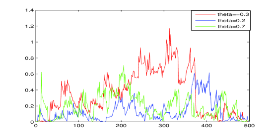
Figure 1: behavior of $T_{n}$ for different values of parameter $\theta$ in MA(1) model

Let $L=1$, therefore corresponding covariance matrix $C=[c_{i,j}]_{i,j=1}^{2}$ can be written as

$$C=\left(\begin{array}[]{cc}2\gamma^{2}(0)+4\gamma^{2}(1)&4\gamma(0)\gamma(1)\\ 4\gamma(0)\gamma(1)&\gamma^{2}(0)+3\gamma^{2}(1)\\ \end{array}\right)=\left(\begin{array}[]{cc}2(1+4\theta^{2}+\theta^{4})&4\theta(1+\theta^{2})\\ 4\theta(1+\theta^{2})&(1+5\theta^{2}+\theta^{4})\\ \end{array}\right)\sigma^{2}.$$

By (2.4), for $t=\frac{k}{n}$ we have that

$$g^{*}_{n}(k/n):=\frac{k}{\sqrt{n}}C^{-1/2}(\hat{\gamma}_{k}(0)-\hat{\gamma}_{n}(0),\,\hat{\gamma}_{k}(1)-\hat{\gamma}_{n}(1))^{T},$$

and by (2.15)

$$T_{n}=\max_{L\leq k<n}\{\frac{k^{2}}{n}(\hat{\gamma}_{k}(0)-\hat{\gamma}_{n}(0),\,\hat{\gamma}_{k}(1)-\hat{\gamma}_{n}(1))C^{-1}(\hat{\gamma}_{k}(0)-\hat{\gamma}_{n}(0),\,\hat{\gamma}_{k}(1)-\hat{\gamma}_{n}(1))^{T}\}.$$

Figure 1 shows the behavior of test statistic $T_{n}$ for different values of parameter $\theta$ in an MA(1) process without change point. For $L=1$, at significant level $\alpha=5\%$, the critical value is $c_{\alpha}=2.408$.

2.2 Consistent estimation of covariance matrix

In this section we evaluate asymptotic behavior of the covariance function of estimators $\hat{\gamma}_{n}(i)$, defined by (2.3). Bartlett(1946) derived an explicit formula for the asymptotic behavior of covariance function of sample autocovariances, when there exist a linear model for the data(Priestley, 1981). We present a consistent estimator $\hat{C}$ for the case that there is no model for data, or we have nonlinear process. Using (2.3), Bartlett’s estimator can be written as:

$$c_{hk}=\lim_{n\rightarrow\infty}\theta_{n}(h,k)=\lim_{n\rightarrow\infty}n\,\mbox{cov}(\hat{\gamma}_{n}(h),\hat{\gamma}_{n}(k)),\ \ 0\leq h\leq k<n.$$

For stationary process $\{X_{t}\}$, let

$$\tilde{\gamma}_{n}(h)=\frac{1}{n}\sum_{t=1}^{n}X_{t}X_{t+h},\ \ 0\leq h<n,$$

and $\tilde{\theta}_{n}(h,k)=n\,\mbox{cov}(\tilde{\gamma}_{n}(h),\tilde{\gamma}_{n}(k))$. By theorem 3 it is shown that $\tilde{\theta}_{n}(h,k)$ has the same asymptotic behavior as $\theta_{n}(h,k)$. For the evaluation of $\tilde{\theta}_{n}(h,k)$, one can easily verify that

$$\tilde{\theta}_{n}(h,k)=n\,\mbox{cov}(\tilde{\gamma}_{n}(h),\tilde{\gamma}_{n}(k))=n\{E(\tilde{\gamma}_{n}(h).\tilde{\gamma}_{n}(k))-\gamma(h).\gamma(k)\}$$

$$=nE\frac{1}{n^{2}}\sum_{t=1}^{n}\sum_{s=1}^{n}\{X_{t}X_{t+h}X_{s}X_{s+k}-\gamma(h)\gamma(k)\}$$

$$=\frac{1}{n}\sum_{t=1}^{n}\sum_{s=1}^{n}E\{X_{t}X_{t+h}X_{s}X_{s+k}-\gamma(h)\gamma(k)\}=\frac{1}{n}\sum_{l=0}^{n-1}\sum_{t=1}^{n-l}\{E(X_{t}X_{t+h}X_{t+l}X_{t+l+k})$$

$$-\gamma(h)\gamma(k)\}+\frac{1}{n}\sum_{l=-n+1}^{-1}\sum_{t=-l+1}^{n}\{E(X_{t}X_{t+h}X_{t+l}X_{t+l+k})-\gamma(h)\gamma(k)\}.$$

By replacing $l$ with $-l$ and $t-l$ with $t$ in last summation we have

$$\tilde{\theta}_{n}(h,k)=\frac{1}{n}\sum_{l=0}^{n-1}\sigma_{h,k}(l),$$

where

$$\sigma_{h,k}(0)=\sum_{t=1}^{n}\{E(X_{t}X_{t+h}X_{t}X_{t+k})-\gamma(h)\gamma(k)\},$$

and for $1\leq l\leq n-1$

$$\sigma_{h,k}(l)=\sum_{t=1}^{n-l}\{E(Y_{1t}^{l})+E(Y_{2t}^{l})-2\gamma(h)\gamma(k)\},$$

in which $Y_{1t}^{l}=X_{t}X_{t+h}X_{t+l}X_{t+l+k}$ and $Y_{2t}^{l}=X_{t+l}X_{t+l+h}X_{t}X_{t+k}$.

Let

$$\bar{\theta}_{n}(h,k)=\frac{1}{n}\sum_{l=0}^{h_{n}}\bar{\sigma}_{h,k}(l),$$

where

$$\bar{\sigma}_{h,k}(0)=\sum_{t=1}^{n}\{\frac{1}{n}\sum_{i=1}^{n}\{Y_{1i}^{0}-\tilde{\gamma}_{n}(h)\tilde{\gamma}_{n}(k)\},\quad\quad\quad$$

$$\bar{\sigma}_{h,k}(l)=\sum_{t=1}^{n-l}\{\frac{1}{n}\sum_{i=1}^{n}\{Y_{1i}^{l}+Y_{2i}^{l}\}-2\tilde{\gamma}_{n}(h)\tilde{\gamma}_{n}(k)\},\quad\quad 1\leq l<n$$

and $\{h_{n}\}$ is a sequence of positive integers that

$$h_{n}=O(n^{\beta})\ \ \;\mbox{for}\ \,\mbox{some}\;\ \beta\in(0,1/2).$$

Now we have the following result.
Theorem 2: Under the assumptions of theorem 1, if  $\sup_{t}E|X_{t}|^{8+\delta}<\infty$ for some $\delta>0$ then

$$\parallel\bar{\theta}_{n}(h,k)-\tilde{\theta}_{n}(h,k)\parallel_{2}\ \rightarrow 0\ \ as\ n\rightarrow\infty.$$

Proof : The proof is organized in three steps:

Step 1: $\lim_{n\rightarrow\infty}\frac{1}{n}\sum_{1\leq l<n}|\sigma_{h,k}(l)|<\infty$.

By lemma 1 and (2.19),

$$|\sigma_{h,k}(l)|\leq|\sum_{t=1}^{n-l}\{E(X_{t}X_{t+h}X_{t+l}X_{t+l+k})-\gamma(h)\gamma(k)\}|+|\sum_{t=1}^{n-l}\{E(X_{t}X_{t+h}X_{t+l}X_{t+l+k})-\gamma(h)\gamma(k)\}|$$

$$\leq\sum_{t=1}^{n-l}[E|X_{t}X_{t+h}|^{p}]^{1/p}[E|X_{t+l}X_{t+l+k}|^{q}]^{1/q}[\alpha(l-h)]^{1-1/p-1/q}+$$

$$\sum_{t=1}^{n-l}[E|X_{t+l}X_{t+l+h}|^{p}]^{1/p}[E|X_{t}X_{t+k}|^{q}]^{1/q}[\alpha(l+h)]^{1-1/p-1/q}.$$

So for $p=q=2+\delta$, by assumption (ii) of theorem 1,

$$|\sigma_{h,k}(l)|\leq M(n-l)\{\alpha_{X}(l-h)^{\frac{\delta}{2+\delta}}+\alpha_{X}(l+h)^{\frac{\delta}{2+\delta}}\},$$

and

$$\lim_{n\rightarrow\infty}\frac{1}{n}\sum_{1\leq l<n}|\sigma_{h,k}(l)|<\infty.$$

Step 2: $\|\bar{\sigma}(l)-\sigma(l)\|_{2}$ is of order $O(n^{1/2})$.
For $1\leq l<n$, by (2.19) and (2.22)

$$\|\sigma_{h,k}(l)-\bar{\sigma}_{h,k}(l)\|_{2}=\|\sum_{t=1}^{n-l}\{EY_{1t}^{l}+EY_{2t}^{l}-2\gamma(h)\gamma(k)\}-\sum_{t=1}^{n-l}\{\frac{1}{n}\sum_{i=1}^{n}Y_{1i}^{l}+\frac{1}{n}\sum_{i=1}^{n}Y_{1i}^{l}-2\tilde{\gamma}_{n}(h)\tilde{\gamma}_{n}(k)\}\|_{2}$$

$$=\|\sum_{t=1}^{n-l}\{EY_{1t}^{l}+EY_{2t}^{l}-2\gamma(h)\gamma(k)-\frac{1}{n}\sum_{i=1}^{n}Y_{1i}^{l}+\frac{1}{n}\sum_{i=1}^{n}Y_{1i}^{l}-2\tilde{\gamma}_{n}(h)\tilde{\gamma}_{n}(k)\}\|_{2}$$

$$\leq\sum_{t=1}^{n-l}\{a_{1}+a_{2}+2a_{3}\},$$

where $a_{1}=\|\frac{1}{n}\sum_{i=1}^{n}\{Y_{1i}^{l}-EY_{1t}^{l}\}\|_{2}$, $a_{2}=\|\frac{1}{n}\sum_{i=1}^{n}\{Y_{2i}^{l}-EY_{2t}^{l}\}\|_{2}$ and $a_{3}=\|\tilde{\gamma}_{n}(h)\tilde{\gamma}_{n}(k)-\gamma(h)\gamma(k)\|_{2}$. As by the assumption of the theorem $\sup_{t}E|Y_{t}|^{2+\delta/4}<\infty$, so by lemma 2

$$a_{1}^{2}=\frac{1}{n^{2}}E(\sum_{i=1}^{n}\{Y_{1i}^{l}-EY_{1t}^{l}\})^{2}=O(n^{-1}),$$

and $a_{1}=O(n^{-1/2})$. Similarly $a_{2}=O(n^{-1/2})$. Also

$$a_{3}=\|\tilde{\gamma}_{n}(h)\tilde{\gamma}_{n}(k)-\gamma(h)\gamma(k)\|_{2}=\|\tilde{\gamma}_{n}(h)\tilde{\gamma}_{n}(k)-\tilde{\gamma}_{n}(h)\gamma(k)+\tilde{\gamma}_{n}(h)\gamma(k)-\gamma(h)\gamma(k)\|_{2}$$

$$\leq\|\tilde{\gamma}_{n}(h)\|_{2}\|\tilde{\gamma}_{n}(k)-\gamma(k)\|_{2}+\|\tilde{\gamma}_{n}(h)-\gamma(h)\|_{2}|\gamma(k)|.$$

Also by lemma 2,

$$\|\tilde{\gamma}_{n}(h)\|_{2}^{2}=\|\frac{1}{n}\sum_{t=1}^{n}X_{t}X_{t+h}\|_{2}^{2}=\frac{1}{n}E(\sum_{t=1}^{n}X_{t}X_{t+h})^{2}<\infty,$$

and

$$\|\tilde{\gamma}_{n}(k)-\gamma(k)\|_{2}^{2}=\|\frac{1}{n}\sum_{t=1}^{n}X_{t}X_{t+h}-\gamma(k)\|_{2}^{2}\leq\frac{1}{n^{2}}E(\sum_{t=1}^{n}X_{t}X_{t+h}-\gamma(k))^{2}=O(n^{-1}).$$

Thus by relations (2.25), (2.26) and (2.27) we have that $a_{3}=O(n^{-1/2})$.
By similar method, one can easily verify that $\|\bar{\sigma}_{h,k}(0)-\sigma_{h,k}(0)\|_{2}=O(n^{1/2})$. Therefore,

$$\|\bar{\sigma}_{h,k}(l)-\sigma_{h,k}(l)\|_{2}\leq O(n^{1/2}).$$

Step 3: Steps 1 and 2 are applied to prove the main result.
By Minkowski inequality we have

$$\|\tilde{\theta}_{n}(h,k)-\bar{\theta}_{n}(h,k)\|_{2}=\|\frac{1}{n}\sum_{l=1}^{n}\sigma_{h,k}(l)-\frac{1}{n}\sum_{l=1}^{h_{n}}\bar{\sigma}_{h,k}(l)\|_{2}\leq$$

$$\frac{1}{n}\sum_{l=1}^{h_{n}}\|\sigma_{h,k}(l)-\bar{\sigma}_{h,k}(l)\|_{2}\ +\frac{1}{n}\sum_{l=h_{n}}^{n}|\sigma_{h,k}(l)|.$$

So by (2.23) and (2.28)

$$\frac{1}{n}\sum_{l=1}^{h_{n}}\|\sigma_{h,k}(l)-\bar{\sigma}_{h,k}(l)\|_{2}\ \leq\frac{1}{n}h_{n}O(n^{1/2})\rightarrow 0,\ \ \ as\ \ n\rightarrow\infty.$$

As $h_{n}\rightarrow\infty$, (2.24) implies that

$$\sum_{h_{n}<l<n}\frac{1}{n}|\sigma_{h,k}(l)|\rightarrow 0,\ \ as\ n\rightarrow\infty.$$

Finally by (2.30) and (2.31), we arrive at the assertion of the theorem. $\Box$

Theorem 3: Under the assumptions of theorem 2, we have that $\|\theta_{n}(h,k)-\bar{\theta}_{n}(h,k)\|_{2}\rightarrow 0,\ as\ n\rightarrow\infty$.
Proof : As

$$\|\theta_{n}(h,k)-\bar{\theta}_{n}(h,k)\|_{2}\leq\|\theta_{n}(h,k)-\tilde{\theta}_{n}(h,k)\|_{2}+\|\tilde{\theta}_{n}(h,k)-\bar{\theta}_{n}(h,k)\|_{2},$$

so by theorem 2 the second part on the right tends to zero, and for the first part, by (2.2) and (2.16)

$$\|\theta_{n}(h,k)-\tilde{\theta}_{n}(h,k)\|_{2}=n\|\mbox{cov}(\hat{\gamma}_{n}(h),\hat{\gamma}_{n}(k))-\mbox{cov}(\tilde{\gamma}_{n}(h),\tilde{\gamma}_{n}(k))\|_{2}$$

$$=\frac{1}{n}\|\sum_{t=1}^{n-h}\sum_{s=1}^{n-k}E\{X_{t}X_{t+h}X_{s}X_{s+k}-\gamma(h)\gamma(k)\}-\sum_{t=1}^{n}\sum_{s=1}^{n}E\{X_{t}X_{t+h}X_{s}X_{s+k}-\gamma(h)\gamma(k)\}\|_{2}$$

$$=\frac{1}{n}\sum_{t=n-h+1}^{n}\sum_{s=n-k+1}^{n}\|\{X_{t}X_{t+h}X_{s}X_{s+k}-\gamma(h)\gamma(k)\}\|_{2}\rightarrow 0,\ \mbox{as}\ n\rightarrow\infty.\Box$$

Corollary 1: Under the assumptions of theorem 2, by choosing $\hat{C}=[\hat{c}_{hk}]_{L+1\times L+1}$, where $\hat{c}_{hk}=\bar{\theta}_{n}(h,k)$ defined by (2.20), $\hat{C}$ is a consistent estimator of covariance matrix $C$ in relation (2.4).

Corollary 2: Under the assumptions of theorem 2, by (2.4), (2.14), (2.15), and corollary 1, we have

$$\hat{T}_{n}=\max_{1\leq k\leq n}\hat{g}^{*}_{n}(k/n)^{T}.\hat{g}^{*}_{n}(k/n)\Rightarrow\sup_{0\leq s\leq 1}\sum_{j=0}^{L}(W^{0}_{j}(s))^{2},$$

where

$$\hat{g}^{*}_{n}(s):=\frac{[ns]}{\sqrt{n}}\hat{C}^{-1/2}(\hat{\gamma}_{[ns]}(0)-\hat{\gamma}_{n}(0),\hat{\gamma}_{[ns]}(1)-\hat{\gamma}_{n}(1),...,\hat{\gamma}_{[ns]}(L)-\hat{\gamma}_{n}(L))^{T},$$

in which $\hat{C}=[\bar{\theta}_{n}(h,k)]$, and $\bar{\theta}_{n}(h,k)$ is defined by (2.20).

3 Simulation results

In this section, we investigate the performance of the proposed test statistic $\hat{T}_{n}$, by a simulation study. As this test statistic is to be applied for linear and nonlinear models, we consider simulations of such classes of time series. Test statistics are evaluated by using relations (2.32) and (2.33) with $L=1$ and relation (2.20) with $h_{n}=n^{0.3}$.

For creating change in the covariance structure of time series, the parameters are changed at the midpoint of the series. Empirical powers are evaluated, and for the case that there is no change in data, probability of type $I$ error is reported.

The critical value of the test statistic at level $\alpha=0.05$ is $c_{\alpha}=2.408$(Lee at el. 2003). Simulations are repeated 1000 times, for the following linear and nonlinear models, to evaluated empirical powers.
Linear models:

• Model 1:
  ARMA(1,1):  $X_{t}-\phi X_{t-1}=Z_{t}+\theta Z_{t-1}$,

• Model 2:
  MA(2):  $X_{t}=Z_{t}+\theta_{1}Z_{t-1}+\theta_{2}Z_{t-2}$,

where $\{Z_{t}\}$ is a sequence of iid normal random variables with mean zero and variance 1.

Table 1: Empirical power of $\hat{T}_{n}$ for ARMA(1,1), where the initial parameter $(\theta_{0},\phi_{0})=(0.1,0.2)$.

	$\phi_{1}$
$\theta_{1}$		0.2		0.4		0.5		0.6
0.1		$0.047^{*}$		0.408		0.761		0.935
0.3		0.295		0.874		0.968		0.989
0.5		0.734		0.977		0.994		0.998
0.7		0.935		0.995		0.999		1.000

Table 1 reports results of the test for simulated data from ARMA(1,1), where 250 samples are generated with $(\theta_{0},\phi_{0})=(0.1,0.2)$, and then 250 more samples for different values of $(\theta_{1},\phi_{1})$ as reported in the table. In table 1, empirical powers are evaluated for cases where one or both parameters have changed. In all cases high empirical powers shows ability of this test statistic. The value pointed by ^∗ is type $I$ error, empirical level, which is slightly below $0.05$.

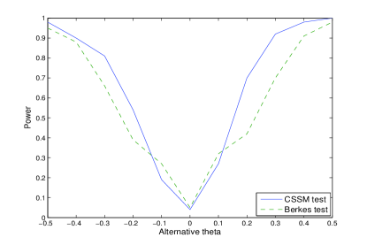
Figure 2: Empirical power of CSSM in comparison with Berkes et al.(2009) in MA(2) model, $X_{t}=Z_{t}+\theta Z_{t-1}+\theta Z_{t-2}$. parameter $\theta$ changes from 0 to alternative $\theta$.

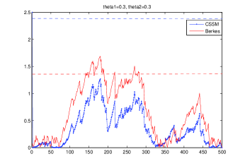
Figure 3: Behavior of CSSM and Berkes statistic in simulated samples from MA(2) model, without change point.

     

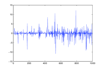
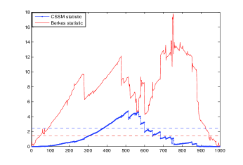
Figure 4: Simulated samples from 2-dependent model with a change point in $k^{*}=500$, variance of $Z_{t}$ change from 1 to 1.26(left), Corresponding test statistics(right).

     

As a comparison of CSSM with the Berkes method for linear models, mode 2 with $\theta=\theta_{1}=\theta_{2}$ is considered and 250 samples are generated with $\theta=0$ at first stage and then 250 more samples for some alternative $\theta$, and empirical powers are plotted in figure 2. As empirical powers show, CSSM test has a better performance, with smaller type $I$ error.

To visualize this, we follow a simulation of model 2, where there is no change in time series data. So we generate 500 samples from MA(2) with $(\theta_{1},\theta_{2})=(0.3,0.3)$ once and again with $(\theta_{1},\theta_{2})=(0.2,0.7)$. Then we evaluate CSSM and Berkes test statistics, and plot them with corresponding critical values, 2.408 and 1.36 in figure 3. As figure 3 shows Berkes method indicate a change point by mistake where CSSM statistic is far beyond such miss detection.
Nonlinear models:

As nonlinear models, we consider followings:

• Model 3:
  2-dependent:  $X_{t}=Z_{t}Z_{t-1}Z_{t-2}$

• Model 4:
  GARCH(1,1):  $X_{t}=h_{t}.Z_{t}$     where   $h_{t}^{2}=\omega+\alpha X^{2}_{t-1}+\beta h_{t-1}^{2}$

in which $\{Z_{t}\}$ is a sequence of iid normal random variables with mean zero and variance one, $\sigma^{2}=1$.

Figure 4(left) shows 1000 generated samples of a 2-dependent process, model 3, with a change point at $k^{*}=500$, where variance of $\{Z_{t}\}$ changes from 1 to 1.26. Figure 4(right) shows the behavior of CSSM and Berkes test statistics. Corresponding critical values are 2.408 and 1.36 respectively which are presented by horizontal lines. Figure 4(right) shows that the supremums of both statistics exceed corresponding critical values and a change in process is detected, but CSSM statistics is more precise, as CSSM detects the change at t=512 and Berkes statistic detects it at t=750.

Table 2 reports the empirical power of the CSSM, for 2-dependent model, model 3. In table 2(a) change of the variance of $\{Z_{t}\}$, from $\sigma^{2}=1$ to alternative values is proposed. In table 2(b) change of the mean of $\{Z_{t}\}$, from $\mu_{0}=0$ to alternative values, has been considered.

Table 2: Empirical power in 2-dependent model.

Table 2(a)		Table 2(b)
change in variance of $Z_{t}$		change in mean of $Z_{t}$
$\sigma$	Power	$\mu$	Power
0.8	0.622	0.0	0.049
0.6	0.960	0.5	0.285
0.4	0.975	1.0	0.961
0.2	0.989	1.5	0.999

Table 3: Empirical power of test in GARCH(1,1) model.

$(\omega,\alpha,\beta)$	n	500		800		1000
no change		0.034		0.035		0.032
(0.8, 0.1, 0.2)		0.528		0.748		0.894
(0.8, 0.1, 0.5)		0.735		0.931		0.967
(0.8, 0.4, 0.2)		0.974		0.999		1.000

Table 3 shows the empirical power of the CSSM statistics in a GARCH(1,1) model. These simulations are done for different values of $n$. Parameters initial values are $(\omega,\alpha,\beta)=(0.5,0.1,0.2)$, and empirical powers for different alternatives are reported. Simulations show that the powers has significant increase with sample size.

4 Conclusion

In this article a nonparametric CUSUM test statistic is proposed for detecting structural changes in strong mixing time series. Under a sufficient condition this test statistic converges in distribution to the supremum of the sum of independent standard Brownian bridges. This method covers a broad class of linear and nonlinear time series such as ARMA and GARCH models, m-dependent models and many others. Beside the wide applications, simulation results shows that our test statistic in comparison with Berkes et al.(2009) has a better performance and is more powerful.

5 Acknowledgment

The authors would like to thank the referee for careful reading of the paper and a number of valuable comments and suggestions that have improved the quality of the paper.

References

[1] Bartlett, M. S. (1946) On the theoretical specification
and sampling properties of autocorrelated time series, J. Royal
Statistical Society 8: 27 41.
[2] Berkes, I., Gombay, E. Horvath, L. (2009).
Testing for changes in the covariance structure of linear
processes, J. Stat. Plan. and Infer. 139:2044-2063.
[3] Billingsley, P. (1999). Convergence of probability measures,
Willey, New York.
[4] Bosq, D. (1996). Nonparametric statistics for stochastic processes,
Springer, New York.
[5] Bradley, R.C. (2005). Basic properties of strong mixing conditions. A survey and
some open questions, Probability Surveys 2:107 144.
[6]
Brockwell, P. Davis, R. Time series: theory and methods, Springer, New York, 1991.
[7] Brodsky, B. E. Darkhovski, B.S. (1993). Nonparametric
methods in change point problems, Kluwer Academic Publishers, Dordrecht.
[8] Csörgö, M. Horváth, L. (1988). Nonparametric methods for change
point problems, In: Krishnaiah, P.R., Rao, C.R. (Eds.), Handbook
of Statistics, Vol. 7. Elsevier, New York, pp. 403-425.
[9] Csörgö, M. Horváth, L. (1997). Limit Theorems in Change-Point
Analysis, Willey, Chichester, UK.
[10] Davydov, Y.A. (1968). Convergence of distributions generated
by stationary stochastic processes, Theor. Probab. Appl. 13:691-696.
[11] Galeano, P. Pena, D. (2007). Covariance changes detection in
multivariate time series, J. Stat. Plan. and Infer. 137:194-211.
[12] Herrndorf, N. (1985). A Functional Central Limit Theorem for Strongly Mixing
Sequences of Random Variables, Z. Wahrscheinlichkeitstheor.
verw. Gebiete 63:97-108.
[13] Ibragimov, I. (1962). Some Limit Theorems for Stationary
Processes, Theory of Probability and Its Applications 7:349-382.
[14] Inclán, C. Tiao, G. C. (1994). Use of cumulative sums of
squares for retrospective detection of changes of variances, J.
Amer. Statist. Assoc. 89:913-923.
[15] Kiefer, J. (1959). K-sample analogues of the Kolmogorov-Smirnov and Cramer-von
Mises tests, Annal. Math. Stat. 30:420-447.
[16] Lee, S. Ha, J. Na, O. Na, S. ( 2003). The cusum test for
parameter change in time series models, Scand. J. Statist. 30:781-796.
[17] Lee, S. Park, S. (2001). The cusum of squares test for scale
changes in infinite order moving average processes, Scand. J.
Statist 28:625-644.
[18] Page, E. S. (1954). Continuous inspection schemes, Biometrika
41:100-115.
[19] Priestley, M. B. (1981). Spectral Analysis and Time Series,
Academic Press, New York.
[20] Qin, R. Tian, Z. Jin, H. Zhang, X. (2010). Strong
convergence rate of robust estimator of change point, Math. Comput. Simul. 80:2026-2032.
[21] Rio, E. (1993). Covariance inequalities for strongly mixing processes,
Ann. Inst. H. Poincare Probab. Statist. 29:587-597.
[22] Romano, J.P., Thombs, L.A. (1996). Inference for autocorrelation
under weak assumptions, J. Amer. Statist. Assoc. 91 (434):590-600.
[23] Zhou, J. Liu, S. Y. (2009). Inference for mean
change-point in infinite variance AR(p) process, Stat. Probab. Lett. 79:6-15.