Gamma-ray flare and absorption in Crab Nebula: Lovely TeV–PeV astrophysics

Abstract

We spectrally fit the GeV gamma-ray flares recently-observed in the Crab Nebula by considering a small blob Lorentz-boosted towards us. We point out that the corresponding inverse-Compton flare at TeV–PeV region is more enhanced than synchrotron by a Lorentz factor square $\sim\Gamma^{2}$, which is already excluding $\Gamma\lower 2.15277pt\hbox{$\;\buildrel>\over{\sim}\;$}200$ and will be detected by future TeV–PeV observatories, CTA, Tibet AS + MD and LHAASO for $\Gamma\lower 2.15277pt\hbox{$\;\buildrel>\over{\sim}\;$}30$. We also show that PeV photons emitted from the Crab Nebula are absorbed by Cosmic Microwave Background radiation through electron-positron pair creation.

1 Introduction

It is well-known that the Crab Nebula is one of the brightest objects in the hard X-ray and gamma-ray sky. Because it was believed that its flux is completely steady, we have used it as a standard candle to calibrate detectors and instruments in those energy ranges. Since the Crab Nebula had already attained a position like a king of strong and steady sources in the high-energy gamma-ray sky, its impermanence must be a historic surprise.

Quite recently AGILE (Tavani et al. 2011) and Fermi ( Abdo et al. 2011; Buehler 2011) reported day-timescale gamma-ray flares from the Crab Nebula in ${\cal O}(10^{2})$MeV– ${\cal O}$(1)GeV region, which means it is no longer stationary. According to the spectral fitting of the stationary component, the flares are most likely produced by synchrotron emission with an increase in the electron energy cutoff $E_{{\rm max},e}\sim$ 10 PeV and/or in magnetic field $B\sim$ 2 $m$G. However, under the standard particle acceleration, the synchrotron energy loss limits the maximum synchrotron photons, irrespective of $B$, below

$$E_{\rm syn}^{\max}\simeq\frac{9}{4}\frac{m_{e}c^{2}}{\alpha}\simeq 160\ {\rm MeV},$$ (1)

which is violated in the flares. Possible solutions include the relativistic Doppler boost (e.g., Komissarov & Lyutikov 2011, Bednarek & Idec 2011, Yuan et al. 2011), the electric-field acceleration in the reconnection layer (e.g., Uzdensky et al. 2011), the sudden concentration of magnetic field (e.g., Bykov et al. 2012), and a DC electric field parallel to the magnetic field (Sturrock & Aschwanden, 2012), but there has been no consensus yet.

In this paper, we consider the relativistic model that a small blob is Lorentz-boosted towards us, which emits synchrotron radiation beyond $E_{\rm syn}^{\max}$ (see Buehler et al. 2011 and references therein). We stress that we can observe the corresponding inverse-Compton flare which is simultaneously emitted by the same electrons existing in the boosted blob. Interestingly, the Lorentz factor $\Gamma$ of the blob has been already constrained by the current TeV observations (Mariotti et al. 2010; Ong et al. 2010) and will be further checked by the future TeV–PeV gamma-ray observations such as CTA, Tibet AS + MD, and LHAASO, because inverse-Compton emission is more enhanced than synchrotron by a factor of $\sim\Gamma^{2}$ approximately. In addition, it is remarkable that we must consider an absorption of PeV photons by Cosmic Microwave Background (CMB) radiation via electron-positron pair creation even for a Galactic source, which has not been taken into account so far. In order to discriminate the theoretical models and discover the new phenomena of the CMB absorption, the Crab Nebula is a pretty attractive experimental site for TeV–PeV astrophysics.

2 Stationary emission from Crab Nebula

2.1 Theory and Observation

First of all, we discuss stationary components of Crab Nebula emission. By assuming a broken power-law with an exponential cutoff for the primary electron spectrum at the emission site, we parameterize it as

$$\frac{dn_{e}}{dE_{e}}=$$

$$A_{e}E_{e}^{-s_{e}}\left(1+\frac{E_{e}}{E_{\rm cb}}\right)^{-1}\left(1+\frac{E_{\rm ib}}{E_{e}}\right)^{-1}\exp\left(-\frac{E_{e}}{E_{{\rm max},e}}\right),$$

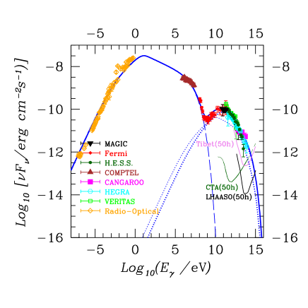
with $n_{e}$ number density of electron, $E_{e}$ electron energy, $E_{{\rm max},e}$ its maximum cutoff energy, $s_{e}$ electron spectral index, $E_{\rm cb}$ the cooling break energy, $E_{\rm ib}$ the intrinsic break energy, and $A_{e}$ normalization. $E_{\rm cb}$ is determined by equating the age $t_{\rm age}$ with cooling time $t_{\rm cool}$ due to the synchrotron energy loss. Here we assume that the exponent of energy on the exponential shoulder is not two but unity (Abdo et al. 2010). The emission below $\sim{\cal O}$(1) GeV can be fitted by synchrotron radiation. The observational data were reported by COMPTEL (Kuiper et al. 2001) and Fermi (Abdo et al. 2010). We adopt values for parameters, $t_{\rm age}$=1240 yrs, $s_{e}=2.35$, magnetic field $B=90\mu$G, the distance to the Earth $d=2.0$ kpc, and the intrinsic breaking energy $E_{\rm ib}=30$ GeV. For the choice of those parameters, e.g., see Abdo et al. (2010) and Tanaka & Takahara (2010). For a reference of the distance, see also Trimble (1973). Then the cooling energy is $E_{\rm cb}=1.3$ TeV, and the cutoff energy is fitted to be $E_{{\rm max},e}=1.5$ PeV. Note that the corresponding synchrotron cutoff energy is $\sim 10$ MeV, but the $\nu F_{\nu}$ peak energy is $\sim$ 4–5 times larger than it because of a finite extent of the distribution.

The emission above $\sim{\cal O}(1)$ GeV can be fitted by inverse-Compton radiation due to the primary electron. Only the number density of the CMB photons is too small and insufficient as target photons to fit the whole data. Besides we also consider the synchrotorn photons and adopt the Synchrotron Self-Compton (SSC) process. In order to obtain target photon field for the SSC process, we integrate the photon number density in a volume where the SSC process occurs. In a one-zone approximation, we find

$$\frac{dn_{\gamma,{\rm target}}}{dE_{\gamma}}=\int\frac{dr}{c}\frac{4\pi d^{2}}{V}\frac{\nu F_{\nu}}{E_{\gamma}^{2}}\sim\frac{d^{2}n_{\gamma,{\rm target}}}{dtdE_{\gamma}}\frac{R_{\rm SSC}}{c},$$ (3)

with $E_{\gamma}$ photon energy, $n_{\gamma,{\rm target}}$ the number density of photon field produced by synchrotron radiation, and $R_{\rm SSC}$ the effective radius where the SSC process works. For similar parameterizations of the effective radius, see Atoyan & Nahapetian (1989), Atoyan & Aharonian (1996), and Tanaka & Takahara (2010). The observational data in $\;\buildrel>\over{\sim}\;$ TeV regions have been reported by MAGIC (Albert et al. 2008), HEGRA (Aharonian et al. 2004), CELESTE (Smith et al. 2006), H.E.S.S. (Aharonian et al. 2006), VERITAS (Celik 2008, Imran et al. 2009), CANGAROO (Tanimori et al. 1998) in addition to Fermi (Abdo et al. 2010), Radio and Optical observations (Baars et al. 1997, Macías-Pérez et al. 2010). To simultaneously fit those data, we find the effective radius to be $R_{\rm SSC}\sim 2.0$ pc. In Fig. 1 we plot the theoretical fitting and the observational data. To perform the fitting we use our original code which has been developed by one of the current authors (KK) in the series of similar works, e.g., Yamazaki et al. (2006).

Figure 1: Spectrum fitted to the stationary component of radiation from Crab Nebula. The solid line shows the total spectrum. The dashed and the dotted lines represent the synchrotron and the inverse-Compton emissions, respectively. The upper and the lower curves of inverse-Compton process at TeV regions are for scattering off the synchrotron and CMB photons, respectively. Observational data are plotted as points with their error bars. We also show sensitivities of future projects such as CTA (Actis et al. 2011) LHAASO (Cao et al. 2010) and Tibet AS + MD (Takita 2011) for 50 hours measurements denoted by (50h).

2.2 PeV gamma-ray absorption by CMB

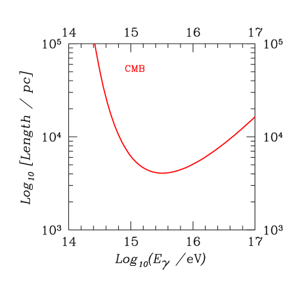
Photon is absorbed if there is a sufficient number of background photons and the electron-positron pair production is kinematically allowed with its energy exceeding threshold $E_{\gamma_{\rm b}}\lower 2.15277pt\hbox{$\;\buildrel>\over{\sim}\;$}m_{e}^{2}c^{4}/(7E_{\gamma})$. The attenuation length is given by

$$L_{\rm atten}(E_{\gamma})=\left[\int dE_{\gamma_{\rm b}}\frac{dn_{\gamma_{\rm b}}}{dE_{\gamma_{\rm b}}}\bar{\sigma}(E_{\gamma},E_{\gamma_{\rm b}})\right]^{-1},$$ (4)

where

$$\bar{\sigma}(E_{\gamma},E_{\gamma_{\rm b}})=\int_{-1}^{1-\frac{2m_{e}^{2}c^{4}}{E_{\gamma}E_{\gamma_{\rm b}}}}d\mu\frac{1-\mu}{2}\sigma_{\rm pair}(E_{\gamma},E_{\gamma_{\rm b}},\mu),$$ (5)

and the pair-production cross section through $\gamma+\gamma\to e^{+}+e^{-}$ is given by

$$\sigma_{\rm pair}(E_{\gamma},E_{\gamma_{\rm b}},\mu)$$

$$= \frac{1}{2}\pi r_{e}^{2}(1-\beta^{2})\left[(3-\beta^{4})\ln\frac{1+\beta}{1-\beta}-2\beta(2-\beta^{2})\right],$$ (6)

with $\beta=\sqrt{1-4m_{e}^{2}c^{4}/s}$ and $s=2E_{\gamma}E_{\gamma_{\rm b}}(1-\mu)$. When we consider a $10^{3}$ TeV ($1$ PeV) photon, the threshold energy of the target photon for the pair production becomes the order of ${\cal O}(10^{-3})$ eV at which the CMB photon dominates along the line of sight between Crab Nebula and the solar system. In Fig. 2 we plot the attenuation length as a function of the photon energy in eV. Remarkably the attenuation length can be down to 4 – 5 kpc at $E_{\gamma}\sim$ (2 – 3) PeV.

Figure 2: Gamma-ray horizon as a function of energy for incident photon. In this energy region, the electron-positron pair production through the scattering off the background CMB photon dominates the energy-loss rate.

Figure 3: Gamma-ray spectra with and without the CMB absorption. We also plotted sensitivities of future projects such as LHAASO (50 h and 100 h), CTA (50 h and 500 h) and Tibet AS + MD (50 h and 500 h) with their observation time, respectively. Note that the vertical axis means $\nu F_{\nu}$ times $E_{\gamma}^{2}$.

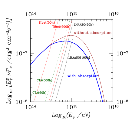
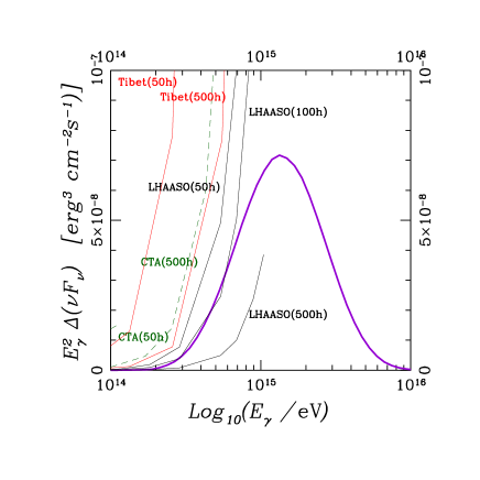
Because the CMB radiation is ideally homogeneous and isotropic, we can simply calculate the absorption factor by using $\exp[-d/L_{{\rm atten}}(E_{\gamma})]$ with $d=2.0$ kpc (Abdo et al. 2010). Multiplying by this absorption factor, we obtain the observed spectrum. In Fig.3 we plot spectra with and without this type of absorption by the CMB radiation. In addition, we also plot sensitivities of future projects such as LHAASO (50 h and 100 h), CTA (50 h and 500 h) and Tibet AS + MD (50 h and 500 h) with their observation time written in round brackets, respectively. In Fig. 4 we compare the observational sensitivities with the net absorbed component, which is the difference between spectra with and without the absorption. From this figure, we find that the absorption by CMB radiation will be observed by LHAASO with its observation time of 100 hours. There could exist inhomogeneities and uncertainies of the target photons. However, by calibrating those photons by using more precise observations within 30 $\%$ at lower eneriges than PeV, we will be able to distinguish the absorption effect from others. In turn, this means that we have to consider this new type of absorption by the CMB radiation whenever we observe the PeV photon from Crab Nebula. As far as we know, we point out this detectability of the PeV photon absorption by the future telescopes for the first time.

Figure 4: Same as Fig. 3 but for the difference between two lines (with and without absorption). Note that the vertical axis means $E_{\gamma}^{2}$ times $\Delta(\nu F_{\nu})$ in linear scale.

3 Fitting to Flare Component

Recently some observations reported that Crab Nebula is no longer stationary with flares at around ${\cal O}$(1) GeV (Tavani et al. 2011, Buehler 2011, Buehler et al. 2011). Fig. 5 shows these data points. The duration $\Delta t_{\rm obs}$ is typically the order of one day. In this section we discuss how we can explain these flares in terms of synchrotron emission by accelerated electrons. We consider Lorentz-boosted blob models in which a small blob is boosted with a Lorentz factor $\Gamma$ and an off-axis viewing angle $\theta$. In addition, as will be discussed later, it should be natural to assume accelerated electrons and magnetic field in the blob. Electrons emit synchrotron radiation by using the local magnetic field in the rest frame of the blob. This model can produce ${\cal O}$(1) GeV synchrotron photon in the observer frame unlike the nonrelativistic models where the synchrotron photon energy cannot exceed $E_{\rm syn}^{\max}\sim 10^{2}$ MeV in equation (1). $E_{\rm syn}^{\max}$ is independent of $B$ because $E_{\rm max,e}$ is limited by balancing synchrotron cooling time with acceleration time. Here we do not specify the origin of the blob, which could be the pulsar wind or the shock at the knot of the inner nebula.

Importantly, inverse-Compton photon is also emitted simultaneously, which is produced by scattering off both the boosted CMB and synchrotron radiation coming from outside the blob. Both of synchrotron and inverse-Compton radiation are boosted-back to the observer frame, which give larger energy and sizably-larger fluxes even if the size of the blob is tiny.

Concretely, the photon energy flux $\nu F_{\nu}$ (in unit of erg cm^-2 s^-1sr^-1) emitted in the rest frame of the blob can be boosted in the observer frame by a following scaling,

$$\nu F_{\nu}(E_{\gamma})\to\delta^{4}\nu F_{\nu}(E_{\gamma}/\delta),$$ (7)

where the Doppler factor is represented by

$$\delta=\frac{1}{\Gamma(1-\beta\cos\theta)},$$ (8)

which behaves like $\sim\Gamma$ for $\theta\lower 2.15277pt\hbox{$\;\buildrel<\over{\sim}\;$}1/\Gamma$, and $\sim 1/\Gamma$ in the other limit for off-axis cases, $\theta\gg 1/\Gamma$. Indeed, this shift of energy for synchrotron emission can fit the change of cutoff scale for the flare component. In addition, for inverse-Compton processes in the rest frame of the blob, the target photon is boosted from the observer frame, and its distribution is modified to be

$$dE_{\gamma}\frac{dn_{\gamma}}{dE_{\gamma}}(E_{\gamma})\to\Gamma dE_{\gamma}\frac{dn_{\gamma}}{dE_{\gamma}}(E_{\gamma}/\Gamma).$$ (9)

Therefore the inverse-Compton power is more enhanced than the synchrotron power by a factor of $\Gamma^{2}$ for the Thomson limit,

$$\frac{(\nu F_{\nu})_{\rm IC}}{(\nu F_{\nu})_{\rm syn}}\to\Gamma^{2}\frac{(\nu F_{\nu})_{\rm IC}}{(\nu F_{\nu})_{\rm syn}}~{}~{}.$$ (10)

Considering the Klein-Nishina effect, the enhancement could be smaller than $\Gamma^{2}$. 

Next we discuss our choice of model parameters. If the maximum energy of electron in the blob rest frame is limited by the synchrotron cooling, the bulk Lorentz factor should be $\lower 2.15277pt\hbox{$\;\buildrel<\over{\sim}\;$}10$ to explain the energy shift of the maximum energy $E_{\rm syn}^{\max}$ shown in equation (1) at the flare. In that case, the synchrotron cooling time should be shorter than the variability timescale, which gives

$$E^{\prime}_{{\rm max},e}>170~{}{\rm TeV}~{}\left(\frac{B^{\prime}}{3~{}{\rm mG}}\right)^{-2}\left(\frac{\delta}{10}\right)^{-1}\left(\frac{\Delta t_{\rm obs}}{8~{}{\rm h}}\right)^{-1}~{}~{},$$ (11)

where $E^{\prime}_{{\rm max},e}$ is the maximum energy of electrons, and $B^{\prime}$ is magnetic field in the rest frame of the blob, respectively.

The Lorentz factor can be larger than $\lower 2.15277pt\hbox{$\;\buildrel>\over{\sim}\;$}10$ because the maximum energy of electrons is not necessarily limited only by cooling, but by the blob size (e.g., Ohira et al. 2011). In this latter case, the Larmor radius of electron with the maximum energy would be comparable to the blob size, $\sim\delta c\Delta t_{\rm obs}$ in the blob rest frame, which gives

$$E^{\prime}_{{\rm max},e}=790~{}{\rm TeV}~{}\left(\frac{B^{\prime}}{3~{}{\rm mG}}\right)\left(\frac{\delta}{10}\right)\left(\frac{\Delta t_{\rm obs}}{8~{}{\rm h}}\right)~{}~{}.$$ (12)

Equating (11) with (12), we obtain a threshold magnetic field in the blob rest frame,

$$B_{\rm th}^{\prime}=1.8~{}{\rm mG}\left(\frac{\delta}{10}\right)^{-2/3}\left(\frac{\Delta t_{\rm obs}}{8~{}{\rm h}}\right)^{-2/3}~{}~{}.$$ (13)

For $B^{\prime}>B_{\rm th}^{\prime}$, the maximum energy of electron is limited by the synchrotron cooling. However, $B_{\rm th}^{\prime}$ is much larger than that expected from the standard model of the steady-state Crab Nebula (e.g. Kennel & Coroniti 1984). Therefore, we also consider the case, $B^{\prime}<B_{\rm th}^{\prime}$, where the maximum energy of electron is limited by the blob size. Because the observed energy of synchrotron photons for a monoenergetic electron is written as

$$E_{\rm syn}=95~{}{\rm MeV}\left(\frac{\delta}{10}\right)\left(\frac{E^{\prime}_{{\rm max},e}}{500~{}{\rm TeV}}\right)^{2}\left(\frac{B^{\prime}}{3~{}{\rm mG}}\right),$$ (14)

by removing $E^{\prime}_{{\rm max},e}$ from Equation (12), the magnetic field in the blob rest frame is obtained as

$$B^{\prime}=2.2~{}{\rm mG}\left(\frac{E_{\rm syn}}{10^{2}~{}{\rm MeV}}\right)^{1/3}\left(\frac{\delta}{10}\right)^{-1}\left(\frac{\Delta t_{\rm obs}}{8~{}{\rm h}}\right)^{-2/3}.$$ (15)

Then the condition $B^{\prime}<B_{\rm th}^{\prime}$ gives lower bound on the Doppler factor

$$\delta>22~{}\left(\frac{E_{\rm syn}}{10^{2}~{}{\rm MeV}}\right).$$ (16)

By removing $\delta$ in (12) with (14), we get the maximum energy of electron in the blob rest frame,

$$E^{\prime}_{{\rm max},e}=480~{}{\rm TeV}\left(\frac{E_{\rm syn}}{10^{2}~{}{\rm MeV}}\right)^{1/2}\left(\frac{\Delta t_{\rm obs}}{8~{}{\rm hours}}\right)^{1/3},$$ (17)

which depends only on observables. In this size-limit case, the variability timescale should be determined by the dynamics of the blob, since the cooling timescale is longer than that. This may be favorable for explaining the comparable timescales of rise and decay in the observed flares.

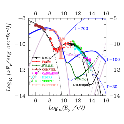
In Fig 5 we plot theoretical calculations of the spectrum fitted to the flare component, adopting a scaling law for magnetic field $B^{\prime}=220\mu{\rm G}(\delta/10^{2})^{-1}$ in equation (15) and the maximum energy of electron obtained in equation (17). The thick solid line shows a result with $\Gamma=\delta=10^{2}$ and $B=223~{}\mu$G. We call this set of parameters “fiducial model”. Because the electrons in the blob cannot be cooled in such a short time, the cooling break does not appear in GeV region. Then the spectral index of electron could be the same as the initial value, $n_{s}\sim$2.35. Consequently the photon index of synchrotron radiation ($F_{\nu}/\nu$) at around ${\cal O}(10^{2})$ MeV becomes $(n_{s}+1)/2\sim 1.6$, which is consistent with the observation ($1.27\pm 0.12$) reported by Buehler (2011). Below ${\cal O}$(10) MeV, the synchrotron flare component is smaller than the stationary one. We also plot the high and low $\Gamma$ models with $\Gamma=\delta=700$ and $\Gamma=\delta=30$ by using the same scaling law for the magnetic field.

On the other hand, in TeV-PeV region, it is remarkable that the inverse-Compton radiation of the flare component can exceed the stationary one significantly at $E_{\gamma}\lower 2.15277pt\hbox{$\;\buildrel>\over{\sim}\;$}{\cal O}(10)$ TeV for the fiducial model. That is also due in part to that the inverse-Compton power is enhanced more than the synchrotron power because of the boosted target photon distribution by a factor of $\Gamma^{2}$ shown in (10). . From Figure 5, we find that higher Lorentz factor than $\Gamma\lower 2.15277pt\hbox{$\;\buildrel>\over{\sim}\;$}700$ has been already excluded by the current GeV observations and $\Gamma\lower 2.15277pt\hbox{$\;\buildrel>\over{\sim}\;$}200$ by TeV observations (Mariotti et al. 2010; Ong et al. 2010).

The future gamma-ray observatories such as CTA, Tibet AS + MD and LHAASO will be able to probe $\Gamma$ down to $\sim 30$ by 8 hours observations (by one night). The sensitivities are shown in Fig. 5 by conservatively linearly scaling them from 50 hours to 8 hours. Even if the flare flux is less than the stationary one, we can detect it down to the statistical error of photons. Note that the ratio of inverse Compton to synchrotron power depends only on $\Gamma$ in equation (10), not on $\delta$, so that we can constraint $\Gamma$ even for an off-axis event. Note also that the cooling effects can be seen a little in $\;\buildrel>\over{\sim}\;$ PeV region for $\Gamma\lower 2.15277pt\hbox{$\;\buildrel<\over{\sim}\;$}$ 30.

To be more conservative, we also show similar calculations with adding an artificial low-energy cutoff for the electron spectrum where we took zero flux for $E_{e}<E_{e,{\rm cut}}=10^{2}$ TeV in the blob rest frame, which is represented by the shallower thick solid lines [this may explain the X-ray feature (Tavani et al. 2011)]. Even in this case, we can probe $\Gamma$ down to $\sim 700$.

Therefore we can discern the model from the nonrelativistic ones for the flares at ${\cal O}$(1) GeV by observing the inverse-Compton radiation in the ${\cal O}$(10)TeV–${\cal O}$(1)PeV energies.

Here it should be meaningful to check an energy ratio of electron to magnetic field in the blob. The flare luminosity in the blob rest frame, $L^{\prime}$, is given by

$$L^{\prime}=4\pi d^{2}(\nu F_{\nu})_{\rm obs}\delta^{-4}~{}~{}.$$ (18)

Assuming that this luminosity is produced by synchrotron radiation of electrons with a typical maximum energy, the luminosity is written as

$$L^{\prime}=N_{\rm e}^{\prime}(E^{\prime}_{{\rm max},e})\times\frac{4}{3}\sigma_{\rm T}c\left(\frac{B^{\prime 2}}{8\pi}\right)\left(\frac{E_{\max,e}^{\prime}}{m_{e}c^{2}}\right)^{2}~{}~{},$$ (19)

where $N_{\rm e}^{\prime}(E^{\prime}_{{\rm max},e})$ is the number of electrons with the maximum energy in the blob rest frame. From Equations (15), (17), (18) and (19), we obtain the total energy of electrons with $E_{\max,e}^{\prime}$,

$$U_{e}^{\prime} = N_{e}^{\prime}(E^{\prime}_{{\rm max},e})E^{\prime}_{\max,e}$$

$$= 1.3\times 10^{37}~{}{\rm erg}~{}\left(\frac{E_{\rm syn}}{10^{2}~{}{\rm MeV}}\right)^{-7/6}\left(\frac{\delta}{10}\right)^{-2}\left(\frac{\Delta t_{\rm obs}}{8~{}{\rm h}}\right).$$

On the other hand, from equation (15), the total energy of the magnetic field in the blob rest frame is given by

$$U_{B}^{\prime} = \frac{B^{\prime 2}}{8\pi}\times\frac{4}{3}\pi\left(\delta c\Delta t_{\rm obs}\right)^{3}$$ (21)

$$= 4.8\times 10^{41}~{}{\rm erg}~{}\left(\frac{E_{\rm syn}}{10^{2}~{}{\rm MeV}}\right)^{2/3}\left(\frac{\delta}{10}\right)\left(\frac{\Delta t_{\rm obs}}{8~{}{\rm h}}\right)^{5/3}.$$ (22)

for the size-limit case $B^{\prime}<B^{\prime}_{\rm th}$. Then, we find the ratio of the electron energy to the magnetic energy to be

$$\frac{U_{e}^{\prime}}{U_{B}^{\prime}}=2.6\times 10^{-5}~{}\left(\frac{E_{\rm syn}}{10^{2}~{}{\rm MeV}}\right)^{-11/6}\left(\frac{\delta}{10}\right)^{-3}\left(\frac{\Delta t_{\rm obs}}{8~{}{\rm h}}\right)^{-2/3}.$$ (23)

This ratio can increase by $\sim(E_{\max,e}/E_{\rm ib})^{n_{s}-2}$ for $2<n_{s}<3$ if we include the low energy electrons. Even in this case, the boosted blob might be magnetically dominant. Since the blob position, $\Gamma\delta c\Delta t_{\rm obs}\sim 8.6\times 10^{14}\Gamma\delta~{}{\rm cm}$, may be also much smaller than the radius of the termination shock, $\sim 3\times 10^{17}~{}{\rm cm}$, the blob might be produced in the pulsar wind before the magnetic energy is converted to the bulk kinetic energy. Alternatively, the observed flares might be off-axis ones with small $\delta(\sim 1)$. In this case we predict larger flares than ever detected. Or a flare may consist of many pulses with $\Delta t_{\rm obs}<8$ h, e.g., $U^{\prime}_{e}\sim U^{\prime}_{B}$ for $\Delta t_{\rm obs}\sim 33$ msec (pulsar period). It may be the reason for the scarcity of flares that a flare needs many pulses (see also Clausen-Brown & Lyutikov 2012).

If we require that the blob energy $\Gamma U^{\prime}_{B}$ is less than the spin-down energy during the flare ${\dot{E}}\Delta t_{\rm obs}\delta/\Gamma$ in the observer frame, we have $\Gamma^{2}\lower 2.15277pt\hbox{$\;\buildrel<\over{\sim}\;$}300(E_{\rm syn}/10^{2}{\rm MeV})^{-2/3}(\Delta t_{\rm obs}/8{\rm h})^{-2/3}$ for the size-limit case $B^{\prime}<B^{\prime}_{\rm th}$. Thus, if we find $\Gamma>30$, we also imply that a flare consists of many pulses with $\Delta t_{\rm obs}<8$ h.

Figure 5: Spectrum fitted to the flare component of radiation from Crab Nebula. We adopted observational data for the flare reported by Fermi (Buehler 2011, Buehler et al. 2011) which is denoted by Fermi2011. The thick solid line shows the theoretical prediction with $\Gamma=\delta=10^{2}$, The thin solid lines are the cases for $\Gamma=\delta=30$ and $\Gamma=\delta=700$, respectively. The corresponding models with low-energy cutoff ($E_{e,{\rm cut}}=10^{2}$ TeV) are represented by the shallower solid lines. The meanings of the other lines and the observational data are the same as those in Fig. 1.

We have not specified the radiation region, which could be the pulsar wind or the shock at the knot of the inner nebula. We have inferred the physical condition and found several possibilities, such as the magnetically dominant case, the off-axis case, and the case of superposition of many pulses, which may be discriminated by future TeV-PeV observations as argued below Eq. (23).

As was mentioned in Introduction, so far there has been no consensus of the theoretical models. In the model with only increasing the maximum energy of electron such as by the electric acceleration, there is surely an excess in PeV region for inverse-Compton flare component. In order to detect this excess by LHAASO, however, we approximately need a few tens of hours for the observation time, which is longer than the typical duration of the flare. In the model with only increasing the magnetic field such as by rapid compression, the inverse-Compton flare is highly suppressed.

4 Summary and Conclusion

In order to explain the origin of the GeV flare in Crab Nebula, we have studied models in which a small blob is boosted, e.g., with a Lorentz factor $\Gamma\lower 2.15277pt\hbox{$\;\buildrel>\over{\sim}\;$}$ $30$, and emits synchrotron photon higher than the maximum synchrotron energy $E_{\rm syn}^{\max}$ shown in equation (1). We have also discussed possibilities that we will discern the model from the others such as nonrelativistic models, by observing the corresponding inverse-Compton flare component. We have pointed out that the inverse-Compton flare can appear in $\lower 2.15277pt\hbox{$\;\buildrel>\over{\sim}\;$}{\cal O}$(1) TeV region accompanied with the GeV flare in this kind of the boosted blob models with large Lorentz factor because the inverse-Compton power is more boosted than the synchrotron power by $\sim\Gamma^{2}$. High $\Gamma$ models have been already excluded for $\Gamma\lower 2.15277pt\hbox{$\;\buildrel>\over{\sim}\;$}200$ by the current TeV observations and will be further down to $\Gamma\sim 30$ by the future TeV–PeV observatories, such as CTA, Tibet AS + MD or LHAASO. In addition, by considering this enhancement in the TeV-PeV region, in near future we may observe “orphan TeV-flares”, which do not have even a GeV flare.

Even for the stationary component of Crab Nebula, we have also pointed out for the first time that the absorption of PeV photons by CMB radiation through pair creation $\gamma+\gamma_{\rm CMB}\to e^{+}+e^{-}$ is important. We must consider this effect whenever we fit the spectrum of Crab Nebula in the ${\cal O}$(1)PeV regions.

It is notable that we will be able to accomplish those studies for observation of Crab Nebula at ${\cal O}$(1)TeV–${\cal O}$(1)PeV energies by using the future gamma-ray telescopes such as CTA, Tibet AS + MD or LHAASO. We hope the earliest possible completions of this kind of new gamma-ray telescopes.

References

- Abdo et al. (2010) Abdo, A. A., et al. 2010, ApJ, 708, 1254
- Abdo et al. (2011) Abdo, A. A., et al. 2011, Science, 331, 739
- Actis et al. (2011) Actis, M., et al. 2011, Experimental Astronomy, 32, 193
- Aharonian et al. (2004) Aharonian, F., et al. 2004, ApJ, 614, 897
- Aharonian et al. (2006) Aharonian, F., et al. 2006, A&A, 457, 899
- Albert et al. (2008) Albert, J., et al. 2008, ApJ, 674, 1037
- Atoyan & Aharonian (1996) Atoyan, A. M., & Aharonian, F. A. 1996, MNRAS, 278, 525
- Atoyan & Nahapetian (1989) Atoyan, A. M., & Nahapetian, A. 1989, A&A, 219, 53
- Baars et al. (1977) Baars, J. W. M., et al. 1977, A&A, 61, 99
- Bednarek & Idec (2011) Bednarek, W., & Idec, W. 2011, MNRAS, 414, 2229
- Buehler (2011) Buehler, R. for the Fermi LAT collaboration, 2011, talk in the Fermi Symposium 2011 (Rome 11th May, 2011)
- Buehler et al. (2011) Buehler, R., et al. 2011, arXiv:1112.1979
- (13) Bykov, A. M., Pavlov, G. G., Artemyev, A. V., & Uvarov, Yu. A. 2012, MNRAS, in press
- Cao et al. (2010) Cao, Z., et al. (LHAASO collaboration) 2010, Chinese Physics C 34(2), 249-252
- Celik (2008) Celik, O. 2008, Ph.D. Thesis, UCLA
- Clausen-Brown & Lyutikov (2012) Clausen-Brown, E., & Lyutikov, M. 2012, arXiv:1205.5094
- Imran & for the VERITAS Collaboration (2009) Imran, A., & for the VERITAS Collaboration 2009, arXiv:0908.0142
- Kennel & Coroniti (1984) Kennel, C. F., & Coroniti, F. V., 1984, ApJ, 283, 694
- Komissarov & Lyutikov (2011) Komissarov, S. S., & Lyutikov, M., 2011, MNRAS, 414, 2017
- Kuiper et al. (2001) Kuiper, L., et al. 2001, A&A, 378, 918
- Macías-Pérez et al. (2010) Macías-Pérez, J. F., et al. 2010, ApJ, 711, 417
- Mariotti et al. (2010) Mariotti, M., et al. 2010, ATel, 2967
- Ohira et al. (2011) Ohira, Y., Yamazaki, R., Kawanaka, N., Ioka, K., arXiv:1106.1810
- Ong et al. (2010) Ong, R. A., et al. 2010, ATel, 2968
- Smith et al. (2006) Smith, D. A., Brion, E., Britto, R., et al. 2006, A&A, 459, 453
- Sturrock & Aschwanden (2012) Sturrock, P., & Aschwanden, M. J. 2012, arXiv:1205.0039
- Takita (2011) Takita, M. on behalf of the Tibet AS + MD Collaboration 2011, CRC Town Meeting Talk, Media Center, Univ. of Tokyo, Kashiwa, Japan, 30th July 2011
- Tanaka & Takahara (2010) Tanaka, S. J., & Takahara, F. 2010, ApJ, 715, 1248
- Tanimori et al. (1998) Tanimori, T., et al. 1998, ApJL, 492, L33
- Tavani et al. (2011) Tavani, M., et al. 2011, Science, 331, 736
- Tluczykont et al. (2011) Tluczykont, M., Hampf, D., Horns, D., et al. 2011, Advances in Space Research, 48, 1935
- Trimble (1973) Trimble, V. 1973, PASP, 85, 579
- (33) Uzdensky, D. A., Cerutti, B., & Begelman, M. C. 2011, ApJ, 737, L40
- Wagner et al. (2009) Wagner, R. M., et al. 2009, arXiv:0912.3742
- Yamazaki et al. (2006) Yamazaki, R., Kohri, K., Bamba, A., Yoshida, T., Tsuribe, T. and Takahara, F. 2006, MNRAS, 371, 1975
- Yuan et al. (2011) Yuan, Q., Yin, P.-F., Wu, X.-F., et al. 2011, ApJL, 730, L15