Hyperspectral Unmixing Overview:
Geometrical, Statistical, and Sparse Regression-Based Approaches
Abstract
Imaging spectrometers measure electromagnetic energy scattered in their instantaneous field view in hundreds or thousands of spectral channels with higher spectral resolution than multispectral cameras. Imaging spectrometers are therefore often referred to as hyperspectral cameras (HSCs). Higher spectral resolution enables material identification via spectroscopic analysis, which facilitates countless applications that require identifying materials in scenarios unsuitable for classical spectroscopic analysis. Due to low spatial resolution of HSCs, microscopic material mixing, and multiple scattering, spectra measured by HSCs are mixtures of spectra of materials in a scene. Thus, accurate estimation requires unmixing. Pixels are assumed to be mixtures of a few materials, called endmembers. Unmixing involves estimating all or some of: the number of endmembers, their spectral signatures, and their abundances at each pixel. Unmixing is a challenging, ill-posed inverse problem because of model inaccuracies, observation noise, environmental conditions, endmember variability, and data set size. Researchers have devised and investigated many models searching for robust, stable, tractable, and accurate unmixing algorithms. This paper presents an overview of unmixing methods from the time of Keshava and Mustard’s unmixing tutorial [1] to the present. Mixing models are first discussed. Signal-subspace, geometrical, statistical, sparsity-based, and spatial-contextual unmixing algorithms are described. Mathematical problems and potential solutions are described. Algorithm characteristics are illustrated experimentally.
I Introduction
Hyperspectral cameras [2, 3, 4, 5, 6, 7, 8, 9, 1, 10, 11] contribute significantly to earth observation and remote sensing[12, 13]. Their potential motivates the development of small, commercial, high spatial and spectral resolution instruments. They have also been used in food safety [14, 15, 16, 17], pharmaceutical process monitoring and quality control [18, 19, 20, 21, 22], and biomedical, industrial, and biometric, and forensic applications [23, 24, 25, 26, 27].
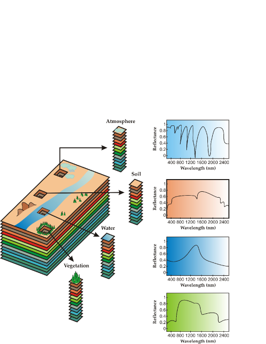
HSCs can be built to function in many regions of the electro-magnetic spectrum. The focus here is on those covering the visible, near-infrared, and shortwave infrared spectral bands (in the range to [5]). Disregarding atmospheric effects, the signal recorded by an HSC at a pixel is a mixture of light scattered by substances located in the field of view [3]. Fig. 1 illustrates the measured data. They are organized into planes forming a data cube. Each plane corresponds to radiance acquired over a spectral band for all pixels. Each spectral vector corresponds to the radiance acquired at a given location for all spectral bands.

I-A Linear and nonlinear mixing models
Hyperspectral unmixing (HU) refers to any process that separates the pixel spectra from a hyperspectral image into a collection of constituent spectra, or spectral signatures, called endmembers and a set of fractional abundances, one set per pixel. The endmembers are generally assumed to represent the pure materials present in the image and the set of abundances, or simply abundances, at each pixel to represent the percentage of each endmember that is present in the pixel.
There are a number of subtleties in this definition. First, the notion of a pure material can be subjective and problem dependent. For example, suppose a hyperspectral image contains spectra measured from bricks laid on the ground, the mortar between the bricks, and two types of plants that are growing through cracks in the brick. One may suppose then that there are four endmembers. However, if the percentage of area that is covered by the mortar is very small then we may not want to have an endmember for mortar. We may just want an endmember for “brick”. It depends on if we have a need to directly measure the proportion of mortar present. If we have need to measure the mortar, then we may not care to distinguish between the plants since they may have similar signatures. On the other hand, suppose that one type of plant is desirable and the other is an invasive plant that needs to be removed. Then we may want two plant endmembers. Furthermore, one may only be interested in the chlorophyll present in the entire scene. Obviously, this discussion can be continued ad nauseum but it is clear that the definition of the endmembers can depend upon the application.
The second subtlety is with the proportions. Most researchers assume that a proportion represents the percentage of material associated with an endmember present in the part of the scene imaged by a particular pixel. Indeed, Hapke [28] states that the abundances in a linear mixture represent the relative area of the corresponding endmember in an imaged region. Lab experiments conducted by some of the authors have confirmed this in a laboratory setting. However, in the nonlinear case, the situation is not as straightforward. For example, calibration objects can sometimes be used to map hyperspectral measurements to reflectance, or at least to relative reflectance. Therefore, the coordinates of the endmembers are approximations to the reflectance of the material, which we may assume for the sake of argument to be accurate. The reflectance is usually not a linear function of the mass of the material nor is it a linear function of the cross-sectional area of the material. A highly reflective, yet small object may dominate a much larger but dark object at a pixel, which may lead to inaccurate estimates of the amount of material present in the region imaged by a pixel, but accurate estimates of the contribution of each material to the reflectivity measured at the pixel. Regardless of these subtleties, the large number of applications of hyperspectral research in the past ten years indicates that current models have value.
Unmixing algorithms currently rely on the expected type of mixing. Mixing models can be characterized as either linear or nonlinear [29, 1]. Linear mixing holds when the mixing scale is macroscopic [30] and the incident light interacts with just one material, as is the case in checkerboard type scenes [31, 32]. In this case, the mixing occurs within the instrument itself. It is due to the fact that the resolution of the instrument is not fine enough. The light from the materials, although almost completely separated, is mixed within the measuring instrument. Fig. 2 depicts linear mixing: Light scattered by three materials in a scene is incident on a detector that measures radiance in bands. The measured spectrum is a weighted average of the material spectra. The relative amount of each material is represented by the associated weight.
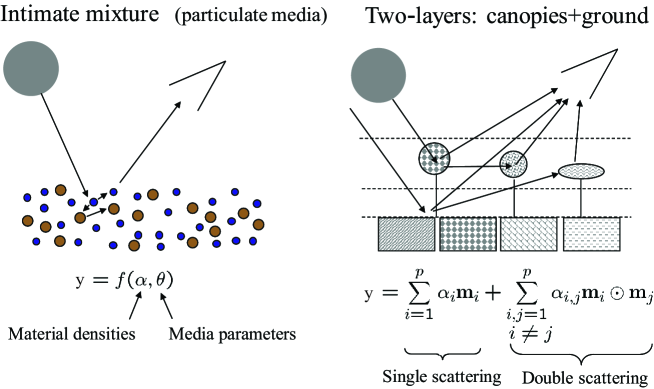
Conversely, nonlinear mixing is usually due to physical interactions between the light scattered by multiple materials in the scene. These interactions can be at a classical, or multilayered, level or at a microscopic, or intimate, level. Mixing at the classical level occurs when light is scattered from one or more objects, is reflected off additional objects, and eventually is measured by hyperspectral imager. A nice illustrative derivation of a multilayer model is given by Borel and Gerstl [33] who show that the model results in an infinite sequence of powers of products of reflectances. Generally, however, the first order terms are sufficient and this leads to the bilinear model. Microscopic mixing occurs when two materials are homogeneously mixed [28]. In this case, the interactions consist of photons emitted from molecules of one material are absorbed by molecules of another material, which may in turn emit more photons. The mixing is modeled by Hapke as occurring at the albedo level and not at the reflectance level. The apparent albedo of the mixture is a linear average of the albedos of the individual substances but the reflectance is a nonlinear function of albedo, thus leading to a different type of nonlinear model.
Fig. 3 illustrates two non-linear mixing scenarios: the left-hand panel represents an intimate mixture, meaning that the materials are in close proximity; the right-hand panel illustrates a multilayered scene, where there are multiple interactions among the scatterers at the different layers.
Most of this overview is devoted to the linear mixing model. The reason is that, despite its simplicity, it is an acceptable approximation of the light scattering mechanisms in many real scenarios. Furthermore, in contrast to nonlinear mixing, the linear mixing model is the basis of a plethora of unmixing models and algorithms spanning back at least 25 years. A sampling can be found in [34, 35, 36, 37, 38, 1, 39, 40, 41, 42, 43, 44, 45, 46, 47]). Others will be discussed throughout the rest of this paper.
I-B Brief overview of nonlinear approaches
Radiative transfer theory (RTT) [48] is a well established mathematical model for the transfer of energy as photons interacts with the materials in the scene. A complete physics based approach to nonlinear unmixing would require inferring the spectral signatures and material densities based on the RTT. Unfortunately, this is an extremely complex ill-posed problem, relying on scene parameters very hard or impossible to obtain. The Hapke [31], Kulbelka-Munk [49] and Shkuratov [50] scattering formulations are three approximations for the analytical solution to the RTT. The former has been widely used to study diffuse reflection spectra in chemistry [51] whereas the later two have been used, for example, in mineral unmixing applications [1, 52].
One wide class of strategies is aimed at avoiding the complex physical models using simpler but physics inspired models, such kernel methods. In [53] and following works [54, 55, 56, 57], Broadwater et al. have proposed several kernel-based unmixing algorithms to specifically account for intimate mixtures. Some of these kernels are designed to be sufficiently flexible to allow several nonlinearity degrees (using, e.g., radial basis functions or polynomials expansions) while others are physics-inspired kernels [55].
Conversely, bilinear models have been successively proposed in [58, 59, 60, 61, 62] to handle scattering effects, e.g., occurring in the multilayered scene. These models generalize the standard linear model by introducing additional interaction terms. They mainly differ from each other by the additivity constraints imposed on the mixing coefficients [63].
However, limitations inherent to the unmixing algorithms that explicitly rely on both models are twofold. Firstly, they are not multipurpose in the sense that those developed to process intimate mixtures are inefficient in the multiple interaction scenario (and vice versa). Secondly, they generally require the prior knowledge of the endmember signatures. If such information is not available, these signatures have to be estimated from the data by using an endmember extraction algorithm.
To achieve flexibility, some have resorted to machine learning strategies such as neural networks [64, 65, 66, 67, 68, 69, 70], to nonlinearly reduce dimensionality or learn model parameters in a supervised fashion from a collection of examples (see [35] and references therein). The polynomial post nonlinear mixing model introduced in [71] seems also to be sufficiently versatile to cover a wide class of nonlinearities. However, again, these algorithms assumes the prior knowledge or extraction of the endmembers.
Mainly due to the difficulty of the issue, very few attempts have been conducted to address the problem of fully unsupervised nonlinear unmixing. One must still concede that a significant contribution has been carried by Heylen et al in [72] where a strategy is introduced to extract endmembers that have been nonlinearly mixed. The algorithmic scheme is similar in many respects to the well-known N-FINDR algorithm [73]. The key idea is to maximize the simplex volume computed with geodesic measures on the data manifold. In this work, exact geodesic distances are approximated by shortest-path distances in a nearest-neighbor graph. Even more recently, same authors have shown in [74] that exact geodesic distances can be derived on any data manifold induced by a nonlinear mixing model, such as the generalized bilinear model introduced in [62].
Quite recently, Close and Gader have devised two methods for fully unsupervised nonlinear unmixing in the case of intimate mixtures [75, 76] based on Hapke’s average albedo model cited above. One method assumes that each pixel is either linearly or nonlinearly mixed. The other assumes that there can be both nonlinear and linear mixing present in a single pixel. The methods were shown to more accurately estimate physical mixing parameters using measurements made by Mustard et al. [77, 64, 57, 56] than existing techniques. There is still a great deal of work to be done, including evaluating the usefulness of combining bilinear models with average albedo models.
In summary, although researchers are beginning to expand more aggressively into nonlinear mixing, the research is immature compared with linear mixing. There has been a tremendous effort in the past decade to solve linear unmixing problems and that is what will be discussed in the rest of this paper.
I-C Hyperspectral unmixing processing chain
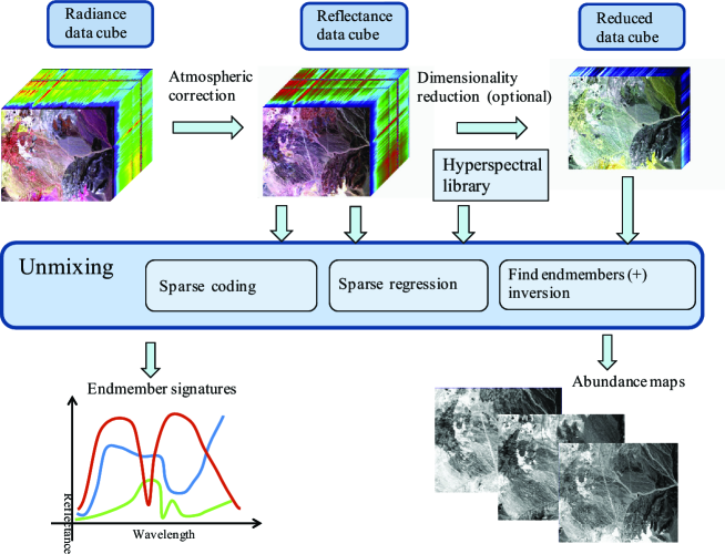
Fig. 4 shows the processing steps usually involved in the hyperspectral unmixing chain: atmospheric correction, dimensionality reduction, and unmixing, which may be tackled via the classical endmember determination plus inversion, or via sparse regression or sparse coding approaches. Often, endmember determination and inversion are implemented simultaneously. Below, we provide a brief characterization of each of these steps:
-
1.
Atmospheric correction. The atmosphere attenuates and scatterers the light and therefore affects the radiance at the sensor. The atmospheric correction compensates for these effects by converting radiance into reflectance, which is an intrinsic property of the materials. We stress, however, that linear unmixing can be carried out directly on radiance data.
-
2.
Data reduction. The dimensionality of the space spanned by spectra from an image is generally much lower than available number of bands. Identifying appropriate subspaces facilitates dimensionality reduction, improving algorithm performance and complexity and data storage. Furthermore, if the linear mixture model is accurate, the signal subspace dimension is one less than equal to the number of endmembers, a crucial figure in hyperspectral unmixing.
-
3.
Unmixing. The unmixing step consists of identifying the endmembers in the scene and the fractional abundances at each pixel. Three general approaches will be discussed here. Geometrical approaches exploit the fact that linearly mixed vectors are in a simplex set or in a positive cone. Statistical approaches focus on using parameter estimation techniques to determine endmember and abundance parameters. Sparse regression approaches, which formulates unmixing as a linear sparse regression problem, in a fashion similar to that of compressive sensing [78, 79]. This framework relies on the existence of spectral libraries usually acquired in laboratory. A step forward, termed sparse coding [80], consists of learning the dictionary from the data and, thus, avoiding not only the need of libraries but also calibration issues related to different conditions under which the libraries and the data were acquired.
-
4.
Inversion. Given the observed spectral vectors and the identified endmembers, the inversion step consists of solving a constrained optimization problem which minimizes the residual between the observed spectral vectors and the linear space spanned by the inferred spectral signatures; the implicit fractional abundances are, very often, constrained to be nonnegative and to sum to one (i.e., they belong to the probability simplex). There are, however, many hyperspectral unmixing approaches in which the endmember determination and inversion steps are implemented simultaneously.
The remainder of the paper is organized as follows. Section 2 describes the linear spectral mixture model adopted as the baseline model in this contribution. Section 3 describes techniques for subspace identification. Sections 4, 5, 6, 7 describe four classes of techniques for endmember and fractional abundances estimation under the linear spectral unmixing. Sections 4 and 5 are devoted to the longstanding geometrical and statistical based approaches, respectively. Sections 6 and 7 are devoted to the recently introduced sparse regression based unmixing and to the exploitation of the spatial contextual information, respectively. Each of these sections introduce the underlying mathematical problem and summarizes state-of-the-art algorithms to address such problem.
Experimental results obtained from simulated and real data sets illustrating the potential and limitations of each class of algorithms are described. The experiments do not constitute an exhaustive comparison. Both code and data for all the experiments described here are available at http://www.lx.it.pt/~bioucas/code/unmixing_overview.zip. The paper concludes with a summary and discussion of plausible future developments in the area of spectral unmixing.
II Linear mixture model
If the multiple scattering among distinct endmembers is negligible and the surface is partitioned according to the fractional abundances, as illustrated in Fig. 2, then the spectrum of each pixel is well approximated by a linear mixture of endmember spectra weighted by the corresponding fractional abundances [3, 29, 39, 1]. In this case, the spectral measurement111Although the type of spectral quantity (radiance, reflectance, etc.) is important when processing data, specification is not necessary to derive the mathematical approaches. at channel ( is the total number of channels) from a given pixel, denoted by , is given by the linear mixing model (LMM)
| (1) |
where denotes the spectral measurement of endmember at the spectral band, denotes the fractional abundance of endmember , denotes an additive perturbation (e.g., noise and modeling errors), and denotes the number of endmembers. At a given pixel, the fractional abundance , as the name suggests, represents the fractional area occupied by the th endmember. Therefore, the fractional abundances are subject to the following constraints:
| (2) |
i.e., the fractional abundance vector (the notation indicates vector transposed) is in the standard -simplex (or unit -simplex). In HU jargon, the nonnegativity and the sum-to-one constraints are termed abundance nonnegativity constraint (ANC) and abundance sum constraint (ASC), respectively. Researchers may sometimes expect that the abundance fractions sum to less than one since an algorithm may not be able to account for every material in a pixel; it is not clear whether it is better to relax the constraint or to simply consider that part of the modeling error.
Let denote a -dimensional column vector, and denote the spectral signature of the th endmember. Expression (1) can then be written as
| (3) |
where is the mixing matrix containing the signatures of the endmembers present in the covered area, and . Assuming that the columns of are affinely independent, i.e., are linearly independent, then the set
i.e., the convex hull of the columns of , is a -simplex in .
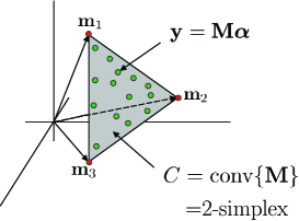
Fig. 5 illustrates a 2-simplex for a hypothetical mixing matrix containing three endmembers. The points in green denote spectral vectors, whereas the points in red are vertices of the simplex and correspond to the endmembers. Note that the inference of the mixing matrix is equivalent to identifying the vertices of the simplex . This geometrical point of view, exploited by many unmixing algorithms, will be further developed in Sections IV-B.
Since many algorithms adopt either a geometrical or a statistical framework [34, 36], they are a focus of this paper. To motivate these two directions, let us consider the three data sets shown in Fig. 6 generated under the linear model given in Eq. 3 where the noise is assumed to be negligible. The spectral vectors generated according to Eq. (3) are in a simplex whose vertices correspond to the endmembers. The left hand side data set contains pure pixels, i.e, for any of the endmembers there is at least one pixel containing only the correspondent material; the data set in the middle does not contain pure pixels but contains at least spectral vectors on each facet. In both data sets (left and middle), the endmembers may by inferred by fitting a minimum volume (MV) simplex to the data; this rather simple and yet powerful idea, introduced by Craig in his seminal work [81], underlies several geometrical based unmixing algorithms. A similar idea was introduced in 1989 by Perczel in the area of Chemometrics et al.[82].
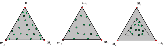
The MV simplex shown in the right hand side example of Fig. 6 is smaller than the true one. This situation corresponds to a highly mixed data set where there are no spectral vectors near the facets. For these classes of problems, we usually resort to the statistical framework in which the estimation of the mixing matrix and of the fractional abundances are formulated as a statistical inference problem by adopting suitable probability models for the variables and parameters involved, namely for the fractional abundances and for the mixing matrix.
II-A Characterization of the Spectral Unmixing Inverse Problem
Given the data set containing -dimensional spectral vectors, the linear HU problem is, with reference to the linear model (3), the estimation of the mixing matrix and of the fractional abundances vectors corresponding to pixels . This is often a difficult inverse problem, because the spectral signatures tend to be strongly correlated, yielding badly-conditioned mixing matrices and, thus, HU estimates can be highly sensitive to noise.
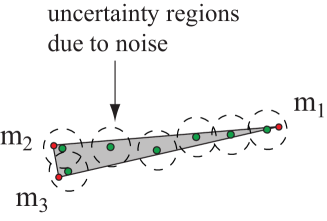
This scenario is illustrated in Fig. 7, where endmembers and are very close, thus yielding a badly-conditioned matrix , and the effect of noise is represented by uncertainty regions.
To characterize the linear HU inverse problem, we use the signal-to-noise-ratio (SNR)
where and are, respectively, the signal (i.e., ) and noise correlation matrices and denotes expected value. Besides SNR, we introduce the signal-to-noise-ratio spectral distribution (SNR-SD) defined as
| (4) |
where is the eigenvalue-eigenvector couple of ordered by decreasing value of . The ratio yields the signal-to-noise ratio (SNR) along the signal direction . Therefore, we must have for , in order to obtain acceptable unmixing results. Otherwise, there are directions in the signal subspace significantly corrupted by noise.
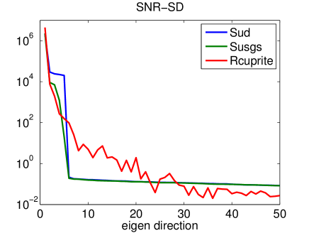
Fig. 8 plots , in the interval , for the following data sets:
-
•
SudP5SNR40: simulated; mixing matrix sampled from a uniformly distributed random variable in the interval ; ; ; fractional abundances distributed uniformly on the 4-unit simplex; SNR40dB.
-
•
SusgsP5SNR40: simulated; mixing matrix sampled from the United States Geological Survey (USGS) spectral library222Available online from: http://speclab.cr.usgs.gov/spectral-lib.html; ; ; fractional abundances distributed uniformly on the 4-unit simplex; SNR40dB.
-
•
Rcuprite: real; subset of the well-known AVIRIS cuprite data cube333Available online from: http://aviris.jpl.nasa.gov/data/free_data.html with size 250 lines by 191 columns by 188 bands (noisy bands were removed).
The signal and noise correlation matrices were obtained with the algorithms and code distributed with HySime [83]. From those plots, we read that, for SudP5SNR40 data set, for and
for , indicating that the SNR
is high in the signal subspace. For SusgsP5SNR40, the singular values of the mixing matrix decay faster due to the high correlation of the USGS spectral signatures. Nevertheless
the “big picture” is similar to that of SudP5SNR40 data set. The Rcuprite data set yields the more difficult inverse problem because has “close to convex shape” slowly approaching the value 1. This is a clear indication of a badly-conditioned inverse problem
[84].
III Signal subspace identification
The number of endmembers present in a given scene is, very often, much smaller than the number of bands . Therefore, assuming that the linear model is a good approximation, spectral vectors lie in or very close to a low-dimensional linear subspace. The identification of this subspace enables low-dimensional yet accurate representation of spectral vectors, thus yielding gains in computational time and complexity, data storage, and SNR. It is usually advantageous and sometimes necessary to operate on data represented in the signal subspace. Therefore, a signal subspace identification algorithm is required as a first processing step.
Unsupervised subspace identification has been approached in many ways. Band selection or band extraction, as the name suggests, exploits the high correlation existing between adjacent bands to select a few spectral components among those with higher SNR [85, 86]. Projection techniques seek for the best subspaces to represent data by optimizing objective functions. For example, principal component analysis (PCA) [87] minimizes sums of squares; singular value decomposition (SVD) [88] maximizes power; projections on the first eigenvectors of the empirical correlation matrix maximize likelihood, if the noise is additive and white and the subspace dimension is known to be [88]; maximum noise fraction (MNF)[89] and noise adjusted principal components (NAPC)[90] minimize the ratio of noise power to signal power. NAPC is mathematically equivalent to MNF [90] and can be interpreted as a sequence of two principal component transforms: the first applies to the noise and the second applies to the transformed data set. MNF is related to SNR-SD introduced in (4). In fact, both metrics are equivalent in the case of white noise, i.e, , where denotes the identity matrix. However, they differ when .
The optical real-time adaptive spectral identification system (ORASIS) [91] framework, developed by U. S. Naval Research Laboratory aiming at real-time data processing, has been used both for dimensionality reduction and endmember extraction. This framework consists of several modules, where the dimension reduction is achieved by identifying a subset of exemplar pixels that convey the variability in a scene. Each new pixel collected from the scene is compared to each exemplar pixel by using an angle metric. The new pixel is added to the exemplar set if it is sufficiently different from each of the existing exemplars. An orthogonal basis is periodically created from the current set of exemplars using a modified Gram-Schmidt procedure [92].
The identification of the signal subspace is a model order inference problem to which information theoretic criteria like the minimum description length (MDL) [93, 94] or the Akaike information criterion (AIC) [95] comes to mind. These criteria have in fact been used in hyperspectral applications [96] adopting the approach introduced by Wax and Kailath in [97]. In turn, Harsanyi, Farrand, and Chang [98] developed a Neyman-Pearson detection theory-based thresholding method (HFC) to determine the number of spectral endmembers in hyperspectral data, referred to in [96] as virtual dimensionality (VD). The HFC method is based on a detector built on the eigenvalues of the sample correlation and covariance matrices. A modified version, termed noise-whitened HFC (NWHFC), includes a noise-whitening step [96]. HySime (hyperspectral signal identification by minimum error) [83] adopts a minimum mean squared error based approach to infer the signal subspace. The method is eigendecomposition based, unsupervised, and fully-automatic (i.e., it does not depend on any tuning parameters). It first estimates the signal and noise correlation matrices and then selects the subset of eigenvalues that best represents the signal subspace in the least square error sense.
When the spectral mixing is nonlinear, the low dimensional subspace of the linear case is often replaced with a low dimensional manifold, a concept defined in the mathematical subject of topology [99]. A variety of local methods exist for estimating manifolds. For example, curvilinear component analysis [100], curvilinear distance analysis [101], manifold learning [102, 103, 104, 105, 106, 107] are non-linear projections based on the preservation of the local topology. Independent component analysis [108, 109], projection pursuit [110, 111], and wavelet decomposition [112, 113] have also been considered.
III-A Projection on the signal subspace
Assume that the signal subspace, denoted by , has been identified by using one of the above referred to methods and let the columns of be an orthonormal basis for , where , for . The coordinates of the orthogonal projection of a spectral vector onto , with respect to the basis , are given by . Replacing by the observation model (3), we have
As referred to before, projecting onto a signal subspace can yield large computational, storage, and SNR gains. The first two are a direct consequence of the fact that in most applications; to briefly explain the latter, let us assume that the noise is zero-mean and has covariance . The mean power of the projected noise term is then ( denotes mean value). The relative attenuation of the noise power implied by the projection is then .
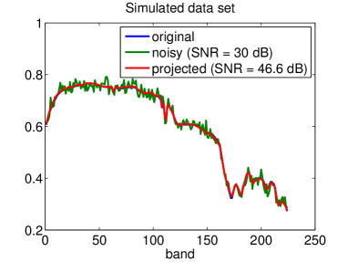
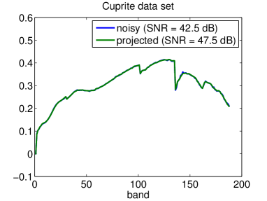
Fig. (9) illustrates the advantages of projecting the data sets on the signal subspace. The noise and the signal subspace were estimated with HySime [83]. The plot on the left hand side shows a noisy and the corresponding projected spectra taken from the simulated data set SusgsP5SNR30444Parameters of the simulated data set SusgsP5SNR30: mixing matrix sampled from a uniformly distributed random variable in the interval ; ; ; fractional abundances distributed uniformly on the 4-unit simplex; SNR40dB.. The subspace dimension was correctly identified. The SNR of the projected data set is dB, which is above to that of the noisy data set. The plot on the right hand side shows a noisy and the corresponding projected spectra from the Rcuprite data set. The identified subspace dimension has dimension 18. The SNR of the projected data set is dB, which is dB above to that of the noisy data set. The colored nature of the additive noise explains the difference dB.


A final word of warning: although the projection of the data set onto the signal subspace often removes a large percentage of the noise, it does not improve the conditioning of the HU inverse problem, as this projection does not change the values of SNR-SD() for the signal subspace eigen-components.
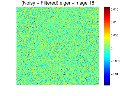
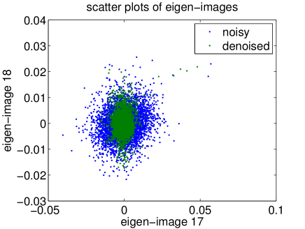
A possible line of attack to further reduce the noise in the signal subspace is to exploit spectral and spatial contextual information. We give a brief illustration in the spatial domain. Fig. 10, on the the top left hand side, shows the eigen-image no. 18, i.e., the image obtained from for , of the Rcuprite data set. The basis of the signal subspace were obtained with the HySime algorithm. A filtered version using then BM3D [114] is shown on the top right hand side. The denoising algorithm is quite effective in this example, as confirmed by the absence of structure in the noise estimate (the difference between the noisy and the denoised images) shown in the bottom left hand side image. This effectiveness can also be perceived from the scatter plots of the noisy (blue dots) and denoised (green dots) eigen-images 17 and 18 shown in the bottom right hand side figure. The scatter plot corresponding to the denoised image is much more dense, reflecting the lower variance.
III-B Affine set projection
From now on, we assume that the observed data set has been projected onto the signal subspace and, for simplicity of notation, we still represent the projected vectors as in (3), that is
| (5) |
where and . Since the columns of belong to the signal subspace, the original mixing matrix is simply given by the matrix product .
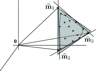
Model (5) is a simplification of reality, as it does not model pixel-to-pixel signature variability. Signature variability has been studied and accounted for in a few unmixing algorithms (see, e.g., [115, 116, 117, 118]), including all statistical algorithms that treat endmembers as distributions. Some of this variability is amplitude-based and therefore primarily characterized by spectral shape invariance [38]; i.e., while the spectral shapes of the endmembers are fairly consistent, their amplitudes are variable. This implies that the endmember signatures are affected by a positive scale factor that varies from pixel to pixel. Hence, instead of one matrix of endmember spectra for the entire scene, there is a matrix of endmember spectra for each pixel = for . In this case, and in the absence of noise, the observed spectral vectors are no longer in a simplex defined by a fixed set of endmembers but rather in the set
| (6) |
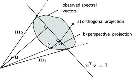
as illustrated in Fig. 11. Therefore, the coefficients of the endmember spectra need not sum-to-one, although they are still nonnegative. Transformations of the data are required to improve the match of the model to reality. If a true mapping from units of radiance to reflectance can be found, then that transformation is sufficient. However, estimating that mapping can be difficult problem or impossible. Other methods can be applied to to ensure that the sum-to-one constraint is a better model, such as the following:
- a)
-
b)
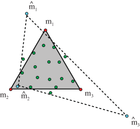
Perspective projection: This is the so-called dark point fixed transform (DPFT) proposed in [81]. For a given observed vector , this projection, illustrated in Fig. 11, amounts to rescale according to , where is chosen such that for every in the data set. The hyperplane containing the projected vectors is defined by , for any .
Notice that the orthogonal projection modifies the direction of the spectral vectors whereas the perspective projection does not. On the other hand, the perspective projection introduces large scale factors, which may become negative, for spectral vectors close to being orthogonal to . Furthermore, vectors with different angles produce non-parallel affine sets and thus different fractional abundances, which implies that the choice of is a critical issue for accurate estimation.
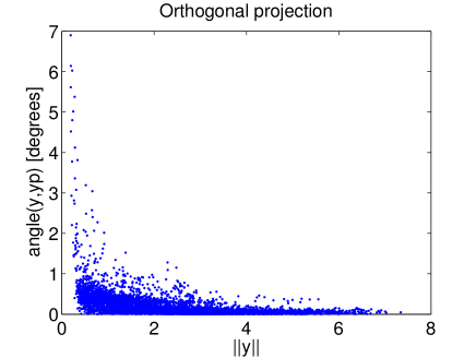
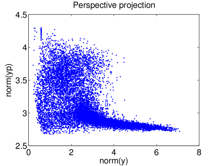
These effects are illustrated in Fig. 12 for the Rterrain data set555http://www.agc.army.mil/hypercube. This is a publicly available hyperspectral data cube distributed by the Army Geospatial Center, United States Army Corps of Engineers, and was collected by the hyperspectral image data collection experiment (HYDICE). Its dimensions are 307 pixels by 500 lines and 210 spectral bands. The figure on the left hand side plots the angles between the unprojected and the orthogonally projected vectors, as a function of the norm of the unprojected vectors. The higher angles, of the order of , occur for vectors of small norm, which usually correspond to shadowed areas. The figure on the right hand side plots the norm of the projected vectors as a function of the norm of the unprojected vectors. The corresponding scale factors varies between, approximately, between 1/3 and 10.
A possible way of mitigating these projection errors is discarding the problematic projections, which are vectors with angles between projected and unprojected vectors larger than a given small threshold, in the case of the perspective projection, and vectors with very small or negative scale factors , in the case of the orthogonal projection.
IV Geometrical based approaches to linear spectral unmixing
The geometrical-based approaches are categorized into two main categories: Pure Pixel (PP) based and Minimum Volume (MV) based. There are a few other approaches that will also be discussed.
IV-A Geometrical based approaches: pure pixel based algorithms
The pure pixel based algorithms still belong to the MV class but assume the presence in the data of at least one pure pixel per endmember, meaning that there is at least one spectral vector on each vertex of the data simplex. This assumption, though enabling the design of very efficient algorithms from the computational point of view, is a strong requisite that may not hold in many datasets. In any case, these algorithms find the set of most pure pixels in the data. They have probably been the most often used in linear hyperspectral unmixing applications, perhaps because of their light computational burden and clear conceptual meaning. Representative algorithms of this class are the following:
-
•
The pixel purity index (PPI) algorithm [120, 121] uses MNF as a preprocessing step to reduce dimensionality and to improve the SNR. PPI projects every spectral vector onto skewers, defined as a large set of random vectors. The points corresponding to extremes, for each skewer direction, are stored. A cumulative account records the number of times each pixel (i.e., a given spectral vector) is found to be an extreme. The pixels with the highest scores are the purest ones.
-
•
N-FINDR [73] is based on the fact that in spectral dimensions, the volume defined by a simplex formed by the purest pixels is larger than any other volume defined by any other combination of pixels. This algorithm finds the set of pixels defining the largest volume by inflating a simplex inside the data.
-
•
The iterative error analysis (IEA) algorithm [122] implements a series of linear constrained unmixings, each time choosing as endmembers those pixels which minimize the remaining error in the unmixed image.
-
•
The vertex component analysis (VCA) algorithm [123] iteratively projects data onto a direction orthogonal to the subspace spanned by the endmembers already determined. The new endmember signature corresponds to the extreme of the projection. The algorithm iterates until all endmembers are exhausted.
-
•
The simplex growing algorithm (SGA) [124] iteratively grows a simplex by finding the vertices corresponding to the maximum volume.
-
•
The sequential maximum angle convex cone (SMACC) algorithm [125] is based on a convex cone for representing the spectral vectors. The algorithm starts with a single endmember and increases incrementally in dimension. A new endmember is identified based on the angle it makes with the existing cone. The data vector making the maximum angle with the existing cone is chosen as the next endmember to enlarge the endmember set. The algorithm terminates when all of the data vectors are within the convex cone, to some tolerance.
- •
-
•
The successive volume maximization (SVMAX) [126] is similar to VCA. The main difference concerns the way data is projected onto a direction orthogonal the subspace spanned by the endmembers already determined. VCA considers a random direction in these subspace, whereas SVMAX considers the complete subspace.
-
•
The collaborative convex framework [128] factorizes the data matrix into a nonnegative mixing matrix and a sparse and also nonnegative abundance matrix . The columns of the mixing matrix are constrained to be columns of the data .
-
•
Lattice Associative Memories (LAM) [129, 130, 131] model sets of spectra as elements of the lattice of partially ordered real-valued vectors. Lattice operations are used to nonlinearly construct LAMS. Endmembers are found by constructing so-called min and max LAMs from spectral pixels. These LAMs contain maximum and minimum coordinates of spectral pixels (after appropriate additive scaling) and are candidate endmembers. Endmembers are selected from the LAMS using the notions of affine independence and similarity measures such as spectral angle, correlation, mutual information, or Chebyschev distance.
Algorithms AVMAX and SVMAX were derived in [126] under a continuous optimization framework inspired by Winter’s maximum volume criterium [73], which underlies N-FINDR. Following a rigorous approach, Chan et al. not only derived AVMAX and SVMAX, but have also unveiled a number of links between apparently disparate algorithms such as N-FINDR and VCA.
IV-B Geometrical based approaches: Minimum volume based algorithms
The MV approaches seek a mixing matrix that minimizes the volume of the simplex defined by its columns, referred to as , subject to the constraint that contains the observed spectral vectors. The constraint can be soft or hard. The pure pixel constraint is no longer enforced, resulting in a much harder nonconvex optimization problem. Fig. 13 further illustrates the concept of simplex of minimum size containing the data. The estimated mixing matrix differs slightly from the true mixing matrix because there are not enough data points per facet (necessarily per facet) to define the true simplex.
Let us assume that the data set has been projected onto the signal subspace , of dimension , and that the vectors , for , are affinely independent (i.e., , for , are linearly independent). The dimensionality of the simplex is therefore so the volume of is zero in . To obtain a nonzero volume, the extended simplex , containing the origin, is usually considered. We recall that the volume of , the convex hull of , is given by
| (7) |
An alternative to (7) consists of shifting the data set to the origin and working in the subspace of dimension . In this case, the volume of the simplex is given by
Craig’s work[81], published in 1994, put forward the seminal concepts regarding the algorithms of MV type. After identifying the subspace and applying projective projection (DPFT), the algorithm iteratively changes one facet of the simplex at a time, holding the others fixed, such that the volume
is minimized and all spectral vectors belong to this simplex; i.e., and (respectively, ANC and ASC constraints666The notation stands for a column vector of ones with size .) for . In a more formal way:
| s.t.: | ||||
| s.t.: |
The minimum volume simplex analysis (MVSA) [132] and the simplex identification via variable splitting and augmented Lagrangian (SISAL) [133] algorithms implement a robust version of the MV concept. The robustness is introduced by allowing the positivity constraint to be violated. To grasp the relevance of this modification, noisy spectral vectors are depicted in Fig. 14. Due to the presence of noise, or any other perturbation source, the spectral vectors may lie outside the true data simplex. The application of a MV algorithm would lead to the dashed estimate, which is far from the original.
In order to estimate endmembers more accurately, MVSA/SISAL allows violations to the positivity constraint. Violations are penalized using the hinge function ( if and if ). MVSA/SISAL project the data onto a signal subspace. Thus the representation of section III-B is used. Consequently, the matrix is square and theoretically invertible (ill-conditioning can make it difficult to compute the inverse numerically). Furthermore,
| (9) |
MVSA/SISAL aims at solving the following optimization problem:
| (10) | |||||
| (11) | |||||
| s.t.: |
where , with being any set of of linearly independent spectral vectors taken from the data set , is a regularization parameter, and stands for the number of spectral vectors.
We make the following two remarks: a) maximizing is equivalent to minimizing ; b) the term weights the ANC violations. As approaches infinity, the soft constraint approaches the hard constraint. MVSA/SISAL optimizes by solving a sequence of convex optimization problems using the method of augmented Lagrange multipliers, resulting in a computationally efficient algorithm.
The minimum volume enclosing simplex (MVES) [134] aims at solving the optimization problem (11) with , i.e., for hard positivity constraints. MVES implements a cyclic minimization using linear programs (LPs). Although the optimization problem (11) is nonconvex, it is proved in (11) that the existence of pure pixels is a sufficient condition for MVES to identify the true endmembers.
A robust version of MVES (RMVES) was recently introduced in [135]. RMVES accounts for the noise effects in the observations by employing chance constraints, which act as soft constraints on the fractional abundances. The chance constraints control the volume of the resulting simplex. Under the Gaussian noise assumption, RMVES infers the mixing matrix and the fractional abundances via alternating optimization involving quadratic programming solvers.
The minimum volume transform-nonnegative matrix factorization (MVC-NMF) [136] solves the following optimization problem applied to the original data set, i.e., without dimensionality reduction:
| (12) | |||||
| s.t.: |
where is a matrix containing the fractional abundances is the Frobenius norm of matrix and is a regularization parameter. The optimization (12) minimizes a two term objective function, where the term measures the approximation error and the term measures the square of the volume of the simplex defined by the columns of . The regularization parameter controls the tradeoff between the reconstruction errors and simplex volumes. MVC-NMF implements a sequence of alternate minimizations with respect to (quadratic programming problem) and with respect to (nonconvex programming problem). The major difference between MVC-NMF and MVSA/SISAL/RMVES algorithms is that the latter allows violations of the ANC, thus bringing robustness to the SU inverse problem, whereas the former does not.

The iterative constrained endmembers (ICE) algorithm [137] aims at solving an optimization problem similar to that of MVC-NMF, where the volume of the simplex is replaced by a much more manageable approximation: the sum of squared distances between all the simplex vertices. This volume regularizer is quadratic and well defined in any ambient dimension and in degenerated simplexes. These are relevant advantages over the regularizer, which is non-convex and prone to complications when the HU problem is badly conditioned or if the number of endmembers is not exactly known. Variations of these ideas have recently been proposed in [138], [139], [140], [141]. ICE implements a sequence of alternate minimizations with respect to and with respect to . An advantage of ICE over MVC-NMF, resulting from the use of a quadratic volume regularizer, is that in the former one minimization is a quadratic programming problem while the other is a least squares problem that can be solved analytically, whereas in the MVC-NMF the optimization with respect to is a nonconvex problem. The sparsity-promoting ICE (SPICE) [142] is an extension of the ICE algorithm that incorporates sparsity-promoting priors aiming at finding the correct number of endmembers. Linear terms are added to the quadratic objective function, one for all the proportions associated with one endmember. The linear term corresponds to an exponential prior. A large number of endmembers are used in the initialization. The prior tends to push all the proportions associated with particular endmembers to zero. If all the proportions corresponding to an endmember go to zero, then that endmember can be discarded. The addition of the sparsity promoting prior does not incur additional complexity to the model as the minimization still involves a quadratic program.
The quadratic volume regularizer used in the ICE and SPICE algorithms also provides robustness in the sense of allowing data points to be outside of the simplex . It has been shown that the ICE objective function can be written in the following way:
where is the sample covariance matrix of the endmembers and is a regularization parameter that controls the tradeoff between error and smaller simplexes. If , then the best solution is to shrink all the endmembers to a single point, so all the data will be outside of the simplex. If , then the best solution is one that yields no error, regardless of the size of the simplex. The solution can be sensitive to the choice of . The SPICE algorithm has the same properties. versions also exist [143].
It is worth noting the both Heylen et al. [144] and Silv n-C rdenas [145] have reported geometric-based methods that can either search for or analytically solve for the fully constrained least squares solution.
The -NMF method introduced in [146] formulates a nonnegative matrix factorization problem similar to (12), where the volume regularizer is replaced with the sparsity-enforcing regularizer . By promoting zero or small abundance fractions, this regularizer pulls endmember facets towards the data cloud having an effect similar to the volume regularizer. The estimates of the endmembers and of the fractional abundances are obtained by a modification of the multiplicative update rules introduced in [147].
Convex cone analysis (CCA) [148], finds the boundary points of the data convex cone (it does not apply affine projection), what is very close to MV concept. CCA starts by selecting the eigenvectors corresponding to the largest eigenvalues. These eigenvectors are then used as a basis to form linear combinations that have only nonnegative elements, thus belonging to a convex cone. The vertices of the convex cone correspond to spectral vectors contains as many zero elements as the number of eigenvectors minus one.
Geometric methods can be extended to piecewise linear mixing models. Imagine the following scenario: An airborne hyperspectral imaging sensor acquires data over an area. Part of the area consists of farmland containing alternating rows of two types of crops (crop A and crop B) separated by soil whereas the other part consists of a village with paved roads, buildings (all with the same types of roofs), and non-deciduous trees. Spectra measured from farmland are almost all linear mixtures of endmember spectra associated with crop A, crop B, and soil. Spectra over the village are almost all linear mixtures of endmember spectra associated with pavement, roofs, and non-deciduous trees. Some pixels from the boundary of the village and farmland may be mixtures of all six endmember spectra. The set of all pixels from the image will then consist of two simplexes. Linear unmixing may find some, perhaps all, of the endmembers. However, the model does not accurately represent the true state of nature. There are two convex regions and the vertices (endmembers) from one of the convex regions may be in the interior of the convex hull of the set of all pixels. In that case, an algorithm designed to find extremal points on or outside the convex hull of the data will not find those endmembers (unless it fails to do what it was designed to do, which can happen). Relying on an algorithm failing to do what it is designed to do is not a desirable strategy. Thus, there is a need to devise methods for identifying multiple simplexes in hyperspectral data. One can refer to this class of algorithms as piecewise convex or piecewise linear unmixing.
One approach to designing such algorithms is to represent the convex regions as clusters. This approach has been taken in [149, 150, 151, 152, 153]. The latter methods are Bayesian and will therefore be discussed in the next section. The first two rely on algorithms derived from fuzzy and possibilistic clustering. Crisp clustering algorithms (such as k-means) assign every data point to one and only one cluster. Fuzzy clustering algorithms allow every data point to be assigned to every cluster to some degree. Fuzzy clusters are defined by these assignments, referred to as membership functions. In the example above, there should be two clusters. Most points should be assigned to one of the two clusters with high degree. Points on the boundary, however, should be assigned to both clusters.
Assuming that there are simplexes in the data, then the following objective function can be used to attempt to find endmember spectra and abundances for each simplex:
| (14) |
such that
Here, represents the membership of the data point in the simplex. The other terms are very similar to those used in the ICE/SPICE algorithms except that there are endmember matrices and abundance vectors. Analytic update formulas can be derived for the memberships, the endmember updates, and the Lagrange multipliers. An update formula can be used to update the fractional abundances but they are sometimes negative and are then clipped at the boundary of the feasible region. One can still use quadratic programming to solve for them. As is the case for almost all clustering algorithms, there are local minima. However, the algorithm using all update formulas is computationally efficient. A robust version also exists that uses a combination of fuzzy and possibilistic clustering [151].
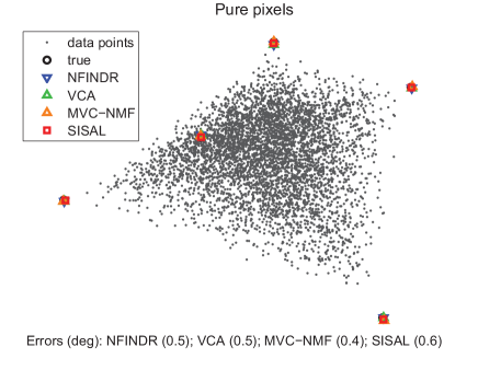
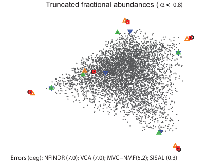
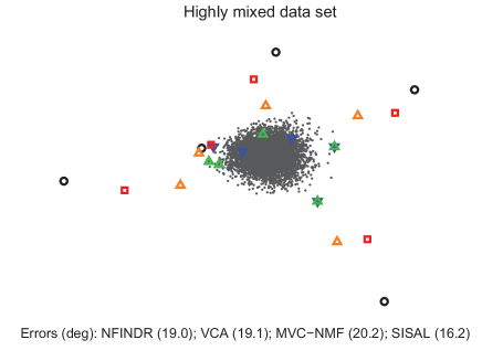
Fig. 15 shows results of pure pixel based algorithms (N-FINDR and VCA) and MV based algorithms (MVC-NMF and SISAL) in simulated data sets representative of the classes of problems illustrated in Fig. 6. These data sets have pixels and SNR = 30 dB and the following characteristics: SusgsP5PPSNR30 - pure pixels and abundances uniformly distributed over the simplex (top left); SusgsP5SNR30 non pure pixels and abundances uniformly distributed over the simplex (top right); SusgsP5MP08SNR30 abundances uniformly distributed over the simplex but truncated to 0.8 (bottom left); SusgsP5XS10SNR30 abundances with Dirichlet distributed with concentration parameter set to 10, thus yielding a highly mixed data set.
In the top left data set all algorithm produced very good results because pure pixels are present. In the top right SISAL and MVC-NMF produce good results but VCA and N-FINDR shows a degradation in performance because there are no pure pixels. In the bottom left SISAL and MVC-NMF still produce good results but VCA and N-FINDR show a significant degradation in performance because the pixels close to the vertices were removed. Finally, in the bottom right all algorithm produce unacceptable results because there are no pixels in the vertex of the simplex neither on its facets. These data sets are beyond the reach of geometrical based algorithms.
V Statistical methods
When the spectral mixtures are highly mixed, the geometrical based methods yields poor results because there are not enough spectral vectors in the simplex facets. In these cases, the statistical methods are a powerful alternative, which, usually, comes with price: higher computational complexity, when compared with the geometrical based approaches. Statistical methods also provide a natural framework for representing variability in endmembers. Under the statistical framework, spectral unmixing is formulated as a statistical inference problem.
Since, in most cases, the number of substances and their reflectances are not known, hyperspectral unmixing falls into the class of blind source separation problems [154]. Independent Component Analysis (ICA), a well-known tool in blind source separation, has been proposed as a tool to blindly unmix hyperspectral data [155, 156, 157]. Unfortunately, ICA is based on the assumption of mutually independent sources (abundance fractions), which is not the case of hyperspectral data, since the sum of abundance fractions is constant, implying statistical dependence among them. This dependence compromises ICA applicability to hyperspectral data as shown in [158, 39]. In fact, ICA finds the endmember signatures by multiplying the spectral vectors with an unmixing matrix which minimizes the mutual information among channels. If sources are independent, ICA provides the correct unmixing, since the minimum of the mutual information corresponds to and only to independent sources. This is no longer true for dependent fractional abundances. Nevertheless, some endmembers may be approximately unmixed. These aspects are addressed in [158].
Bayesian approaches have the ability to model statistical variability and to impose priors that can constrain solutions to physically meaningful ranges and regularize solutions. The latter property is generally considered to be a requirement for solving ill-posed problems. Adopting a Bayesian framework, the inference engine is the posterior density of the random quantities to be estimated. When the unknown mixing matrix and the abundance fraction matrix are assumed to be a priori independent, the Bayes paradigm allows the joint posterior of and to be computed as
| (15) |
where the notation and stands for the probability density function (pdf) of and of given , respectively. In (15), is the likelihood function depending on the observation model and the prior distribution and summarize the prior knowledge regarding these unknown parameters.
A popular Bayesian estimator is [159] the joint maximum a posteriori (MAP) estimator given by
| (16) | |||||
| (17) |
Under the linear mixing model and assuming the noise random vector is Gaussian with covariance matrix , then, we have . It is then clear that ICE/SPICE [142] and MVC-NMF [136] algorithms, which have been classified as geometrical, can also be classified as statistical, yielding joint MAP estimates in (16). In all these algorithms, the estimates are obtained by minimizing a two-term objective function: plays the role of a data fitting criterion and consists of a penalization. Conversely, from a Bayesian perspective, assigning prior distributions and to the endmember and abundance matrices and , respectively, is a convenient way to ensure physical constraints inherent to the observation model.
The work [160] introduces a Bayesian approach where the linear mixing model with zero-mean white Gaussian noise of covariance is assumed, the fractional abundances are uniformly distributed on the simplex, and the prior on is an autoregressive model. Maximization of the negative log-posterior distribution is then conducted in an iterative scheme. Maximization with respect to the abundance coefficients is formulated as weighted least square problems with linear constraints that are solved separately. Optimization with respect to is conducted using a gradient-based descent.
The Bayesian approaches introduced in [161, 162, 163, 164] have all the same flavor. The posterior distribution of the parameters of interest is computed from the linear mixing model within a hierarchical Bayesian model, where conjugate prior distributions are chosen for some unknown parameters to account for physical constraints. The hyperparameters involved in the definition of the parameter priors are then assigned non-informative priors and are jointly estimated from the full posterior of the parameters and hyperparameters. Due to the complexity of the resulting joint posterior, deriving closed-form expressions of the MAP estimates or designing an optimization scheme to approximate them remain impossible. As an alternative, Markov chain Monte Carlo algorithms are proposed to generate samples that are asymptotically distributed according to the target posterior distribution. These samples are then used to approximate the minimum mean square error (MMSE) (or posterior mean) estimators of the unknown parameters
| (18) | |||||
| (19) |
These algorithms mainly differ by the choice of the priors assigned to the unknown parameters. More precisely, in [161, 165], spectral unmixing is conducted for spectrochemical analysis. Because of the sparse nature of the chemical spectral components, independent Gamma distributions are elected as priors for the spectra. The mixing coefficients are assumed to be non-negative without any sum-to-one constraint. Interest of including this additivity constraint for this specific application is investigated in [162] where uniform distributions over the admissible simplex are assigned as priors for the abundance vectors. Note that efficient implementations of both algorithms for operational applications are presented in [166] and [167], respectively.
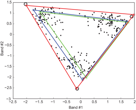
In [163], instead of estimating the endmember spectra in the full hyperspectral space, Dobigeon et al. propose to estimate their projections onto an appropriate lower dimensional subspace that has been previously identified by one of the dimension reduction technique described in paragraph III-A. The main advantage of this approach is to reduce the number of degrees of freedom of the model parameters relative to other approaches, e.g., [161, 165, 162]. Accuracy and performance of this Bayesian unmixing algorithm when compared to standard geometrical based approaches is depicted in Fig. 16 where a synthetic toy example has been considered. This example is particularly illustrative since it is composed of a small dataset where the pure pixel assumption is not fulfilled. Consequently, the geometrical based approaches that attempt to maximize the simplex volume (e.g., VCA and N-FINDR) fail to recover the endmembers correctly, contrary to the statistical algorithm that does not require such hypothesis.
.
Note that in [162], [163] and [164] independent uniform distributions over the admissible simplex are chosen as prior distributions for the abundance vectors. This assumption, which is equivalent of choosing Dirichlet distributions with all hyperparameters equal to , could seem to be very weak. However, as demonstrated in [163], this choice favors estimated endmembers that span a simplex of minimum volume, which is precisely the founding characteristics of some geometrical based unmixing approaches detailed in paragraph IV-B.
Explicitly constraining the volume of the simplex formed by the estimated endmembers has also been considered in [164]. According to the optimization perspective suggested above, penalizing the volume of the recovered simplex can be conducted by choosing an appropriate negative log-prior . Arngren et al. have investigated three measures of this volume: exact simplex volume, distance between vertices, volume of a corresponding parallelepiped. The resulting techniques can thus be considered as stochastic implementations of the MVC-NMF algorithm [136].
All the Bayesian unmixing algorithms introduced above rely on the assumption of an independent and identically Gaussian distributed noise, leading to a covariance matrix of the noise vector . Note that the case of a colored Gaussian noise with unknown covariance matrix has been handled in [168]. However, in many applications, the additive noise term may neglected because the noise power is very small. When that is not the case but the signal subspace has much lower dimension than the number of bands, then, as seen in Section III-A, the projection onto the signal subspace largely reduces the noise power. Under this circumstance, and assuming that is invertible and the observed spectral vectors are independent, then we can write
where is the fractional abundance pdf, and compute the em maximum likelihood (ML) estimate of . This is precisely the ICA line of attack, under the assumption that the fractional abundances are independent, i.e., . The fact that this assumption is not valid in hyperspectral applications [158] has promoted research on suitable statistical models for hyperspectral fractional abundances and in effective algorithms to infer the mixing matrices. This is the case with DECA [169, 170]; the abundance fractions are modeled as mixtures of Dirichlet densities, thus, automatically enforcing the constraints on abundance fractions imposed by the acquisition process, namely nonnegativity and constant sum. A cyclic minimization algorithm is developed where: 1) the number of Dirichlet modes is inferred based on the minimum description length (MDL) principle; 2) a generalized expectation maximization (GEM) algorithm is derived to infer the model parameters; 3) a sequence of augmented Lagrangian based optimizations are used to compute the signatures of the endmembers.
Piecewise convex unmixing, mentioned in the geometrical approaches section, has also been investigated using a Bayesian approach777It is an interesting to remark that by taking the negative of the logarithm of a fuzzy clustering objective function, such as in Eq. 14, one can represent a fuzzy clustering objective as a Bayesian MAP objective. One interesting difference is that the precisions on the likelihood functions are the memberships and are data point dependent. In [171] the normal compositional model is used to represent each convex set as a set of samples from a collection of random variables. The endmembers are represented as Gaussians. Abundance multinomials are represented by Dirichlet distributions. To form a Bayesian model, priors are used for the parameters of the distributions. Thus, the data generation model consists of two stages. In the first stage, endmembers are sampled from their respective Gaussians. In the second stage, for each pixel, an abundance multinomial is sampled from a Dirichlet distribution. Since the number of convex sets is unknown, the Dirichlet process mixture model is used to identify the number of clusters while simultaneously learning the parameters of the endmember and abundance distributions. This model is very general and can represent very complex data sets. The Dirichlet process uses a Metropolis-within-Gibbs method to estimate the parameters, which can be quite time consuming. The advantage is that the sampler will converge to the joint distribution of the parameters, which means that one can select the maximum a-posterior estimates from the estimated joint distributions. Although Gibbs samplers seem inherently sequential, some surprising new theoretical results by [172] show that theoretically correct sampling samplers can be implemented in parallel, which offers the promise of dramatic speed-ups of algorithms such as this and other probabilistic algorithms mentioned here that rely on sampling.
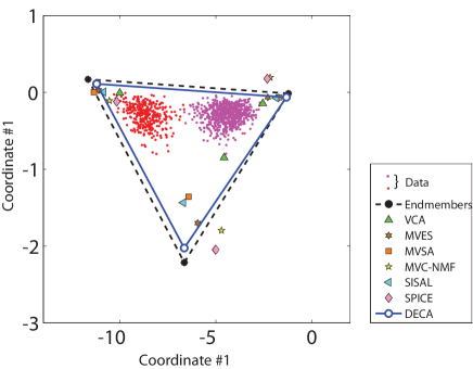

Fig. 17, left, presents a scatterplot of the simulated data set SusgsP3SNRinfXSmix and the endmember estimates produced by VCA, MVES, MVSA, MVC-NMF, SISAL, and DECA algorithms. This data set is generated with a mixing matrix sampled from the USGS library and with endmembers, spectral vectors, and fractional abundances given by mixtures of two Dirichlet modes with parameters and and mode weights of 0.67 and 0.33, respectively. DECA Dirichlet parameters were randomly initialized and the mixing probabilities uniformly. This setting reflects a situation in which no knowledge of the size and the number of regions in the scene exists. The parameters of the remaining methods were hand tuned for optimal performance888MVC-MNF regularization parameter: ; MVES tolerance: ; SISAL regularization parameter ; SPICE regularization parameter ; SPICE sparsity parameter ; SPICE stopping parameter .. See [170] for more details. The considered data set corresponds to a highly mixed scenario, where the geometrical based algorithms performs poorly, as explained in Section IV. On the contrary, DECA yields useful estimates.
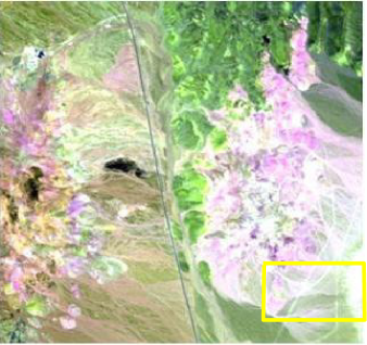
Fig. 17, right, is similar the one in the left hand side for a Cuprite data subset of size pixels shown in Fig. 18. This subset is dominated by Montmorillonite, Desert Varnish, and Alunite, which are known to dominate the considered subset image [6]. The projections of this endmembers are represented by black circles. DECA identified modes, with parameters , , , , and , and mode weights , , , , and . These parameters correspond to a highly non-uniform distribution over the simplex as could be inferred from the scatterplot. Although the estimation results are more difficult to judge in the case of real data than in the case on simulated data, as we not really sure about the true endmembers, it is reasonable to conclude that the statistical approach is producing similar to or better estimates than the geometrical based algorithms.
The examples shown Fig. 17 illustrates the potential and flexibility of the Bayesian methodology. As already referred to above, these advantages come at a price: computational complexity linked to the posterior computation and to the inference of the estimates.
VI Sparse regression based unmixing
The spectral unmixing problem has recently been approached in a semi-supervised fashion, by assuming that the observed image signatures can be expressed in the form of linear combinations of a number of pure spectral signatures known in advance[173, 174, 175] (e.g., spectra collected on the ground by a field spectro-radiometer). Unmixing then amounts to finding the optimal subset of signatures in a (potentially very large) spectral library that can best model each mixed pixel in the scene. In practice, this is a combinatorial problem which calls for efficient linear sparse regression techniques based on sparsity-inducing regularizers, since the number of endmembers participating in a mixed pixel is usually very small compared with the (ever-growing) dimensionality and availability of spectral libraries [1]. Linear sparse regression is an area of very active research with strong links to compressed sensing [176, 79, 177], least angle regression [178], basis pursuit, basis pursuit denoising [179], and matching pursuit [180], [181].
Let us assume then that the spectral endmembers used to solve the mixture problem are no longer extracted nor generated using the original hyperspectral data as input, but instead selected from a library containing a large number of spectral samples, say , available a priori. In this case, unmixing amounts to finding the optimal subset of samples in the library that can best model each mixed pixel in the scene. Usually, we have and therefore the linear problem at hands is underdetermined. Let denote the fractional abundance vector with regards to the library . With these definitions in place, we can now write our sparse regression problem as
| (20) |
where denotes the number of non-zero components of and is the error tolerance due to noise and modeling errors. Assume for a while that . If the system of linear equations has a solution satisfying , where is the smallest number of linearly dependent columns of , it is necessarily the unique solution of [182]. For , the concept of uniqueness of the sparsest solution is replaced with the concept of stability [176].
In most HU applications, we do have and therefore, at least in noiseless scenarios, the solutions of (20) are unique. However, problem (20) is NP-hard [183] and therefore there is no hope in solving it in a straightforward way. Greedy algorithms such as the orthogonal matching pursuit (OMP) [181] and convex approximations replacing the the norm with the norm, termed basis pursuit (BP), if , and basis pursuit denoising (BPDN )[179], if , are alternative approaches to compute the sparsest solution. If we add the ANC to BP and BPDN problems, we have the constrained basis pursuit (CBP) and the constrained basis pursuit denoising (CBPDN) problems [184], respectively. The CBPDN optimization problem is thus
| (21) |
An equivalent formulation to (21), termed constrained sparse regression (CSR) (see [184]), is
| (22) |
where is related with the Lagrange multiplier of the inequality , also interpretable as a regularization parameter.
Contrary to the problem (20), problems (21) and (22) are convex and can be solved efficiently [184, 185]. What is, perhaps, totally unexpected is that sparse vector of fractional abundances can be reconstructed by solving (21) or (22) provided that the columns of matrix are incoherent in a given sense [186]. The applicability of sparse regression to HU was studied in detail in [173]. Two main conclusions were drawn:
- a)
-
hyperspectral signatures tend to be highly correlated what imposes limits to the quality of the results provided by solving CBPDN or CSR optimization problems.
- b)
-
The limitation imposed by the highly correlation of the spectral signatures is mitigated by the high level of sparsity most often observed in the hyperspectral mixtures.
At this point, we make a brief comment about the role of ASC in the context of CBPDN and of CSR problems. Notice that if belongs to the unit simplex (i.e., for , and ), we have . Therefore, if we add the sum-to-one constraint to (21) and (22), the corresponding optimization problems do not depend on the norm . In this case, the optimization (22) is converted into the well known fully constrained least squares (FCLS) problem and (21) into a feasibility problem, which for is
| (23) |
The uniqueness of sparse solutions to (23) when the system is underdetermined is addressed in [187]. The main finding is that for matrices with a row-span intersecting the positive orthant (this is the case of hyperspectral libraries), if this problem admits a sufficiently sparse solution, it is necessarily unique. It is remarkable how the ANC alone acts as a sparsity-inducing regularizer.
In practice, and for the reasons pointed Section III-B, the ASC is rarely satisfied. For this reason, and also due to the presence of noise and model mismatches, we have observed that the CBPDN and CSR often yields better unmixing results than CLS and FCLS.
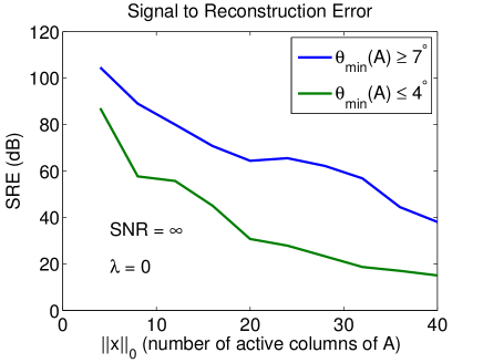

In order to illustrate the potential of the sparse regression methods, we run an experiment with simulated data. The hyperspectral library , of size and , is a pruned version of the USGS library in which the angle between any two spectral signatures is no less than rad (approximately 3 degrees). The abundance fractions follows a Dirichlet distribution with constant parameter of value 2, yielding a mixed data set beyond the reach of geometrical algorithms. In order to put in evidence the impact of the angles between the library vectors, and therefore the mutual coherence of the library [187], in the unmixing results, we organize the library into two subsets; the minimum angle between any two spectral signatures is higher the degrees in the first set and lower than in the second set.
Fig. 19 top, plots unmixing results obtained by solving the CSR problem (22) with the SUNSAL algorithm introduced in [184]. The regularization parameter was hand tuned for optimal performance. For each value of the abscissa , representing the number of active columns of , we select elements of one of the subsets above referred to and generate Dirichlet distributed mixtures. From the sparse regression results, we estimate the signal-to-reconstruction error (SRE) as
where and stand for estimated abundance fraction vector and sample average, respectively.
The curves on the top left hand side were obtained with the noise set to zero. As expected there is a degradation of performance as increases and decreases. Anyway, the obtained values of SRE correspond to an almost perfect reconstruction for . For the reconstruction is almost perfect for , as well, and of good quality for most unmixing purposes for for .
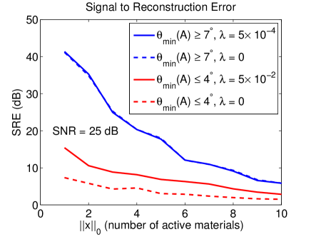
The curves on the top right hand side were obtained with SNRdB. This scenario is much more challenging than the previous one. Anyway, even for , we get SRE dB for, , corresponding to a useful performance in HU applications. Notice that best values of SRE for are obtained with , putting in evidence the regularization effect of the norm in the CSR problem (22), namely when the spectral are strongly coherent.
The curves on the bottom plot the number of incorrect selected materials for SNRdB. This number is zero for SNR. For each value of , we compare the larger elements of with the true ones and count the number of mismatches. We conclude that a suitable setting of the regularization
parameter yields a correct selection of the materials for .
The success of hyperspectral sparse regression relies crucially on the availability of suitable hyperspectral libraries. The acquisition of these libraries is often a time consuming and expensive procedure. Furthermore, because the libraries are hardly acquired under the same conditions of the data sets under consideration, a delicate calibration procedure have to be carried out to adapt either the library to the data set or vice versa [173]. A way to sidestep these difficulties is the learning of the libraries directly from the dataset with no other a priori information involved. For the application of these ideas, frequetly termed dictionary learning, in signal and image processing see, e.g.,, [188, 189] and references therein). Charles et al. have recently applied this line of attack to sparse HU in [190]. They have modified an existing unsupervised learning algorithm to learn an optimal library under the sparse representation moldel. Using this learned library they have shown that the sparse representation model learns spectral signatures of materials in the scene and locally approximates nonlinear manifolds for individual materials.
VII Spatial-spectral contextual information
Most of the unmixing strategies presented in the previous paragraphs
are based on a objective criterion generally defined in the
hyperspectral space. When formulated as an optimization problem
(e.g., implemented by the geometrical-based algorithms detailed in
Section IV), spectral unmixing usually relies on
algebraic constraints that are inherent to the observation space
: positivity, additivity and minimum volume.
Similarly, the statistical- and sparsity-based algorithms of
Sections V and VI
exploit similar geometric constraints to penalize a standard
data-fitting term (expressed as a likelihood function or quadratic
error term). As a direct consequence, all these algorithms ignore
any additional contextual information that could improve the
unmixing process. However, such valuable information can be of great
benefit for analyzing hyperspectral data. Indeed, as a prototypal
task, thematic classification of hyperspectral images has recently
motivated the development of a new class of algorithms that exploit
both the spatial and spectral features contained in image. Pixels
are no longer processed individually but the intrinsic D nature
of the hyperspectral data cube is capitalized by taking advantage of
the correlations between spatial and spectral neighbors (see, e.g.
[191, 192, 193, 194, 195, 196, 197, 198]).
Following this idea, some unmixing methods have targeted the integration of contextual information to guide the endmember extraction and/or the abundance estimation steps. In particular, the Bayesian estimation setting introduced in Section V provides a relevant framework for exploiting spatial information. Anecdotally, one of the earliest work dealing with linear unmixing of multi-band images (casted as a soft classification problem) explicitly attempts to highlight spatial correlations between neighboring pixels. In [199], abundance dependencies are modeled using Gaussian Markov random fields, which makes this approach particularly well adapted to unmix images with smooth abundance transition throughout the observed scene.
In a similar fashion, Eches et al. have proposed to exploit
the pixel correlations by using an underlying membership process.
The image is partitioned into regions where the statistical
properties of the abundance coefficients are homogeneous
[200]. A Potts-Markov random field has been assigned
to hidden labeling variables to model spatial dependencies between
pixels within any region. It is worthy to note that, conditionally
upon a given class, unmixing is performed on each pixel individually
and thus generalizes the Bayesian algorithms of [201].
In [200], the number of homogeneous regions that
compose the image must be chosen and fixed a priori. An
extension to a fully unsupervised method, based on nonparametric
hidden Markov models, have been suggested by Mittelman et al.
in [202].
Several attempts to exploit spatial information have been also made
when designing appropriate criteria to be optimized. In addition to
the classical positivity, full additivity and minimum volume
constraints, other penalizing terms can be included in the objective
function to take advantage of the spatial structures in the image.
In [203], the spatial autocorrelation of each abundance
is described by a measure of spatial complexity, promoting these
fractions to vary smoothly from one pixel to its neighbors (as in
[199]). Similarly, in [204], spatial
information has been incorporated within the criterion by including
a regularization term that takes into account a weighted combination
of the abundances related to the neighboring pixels. Other
optimization algorithms operate following the same strategy (see for
examples [205, 206, 207]).
Extended morphological operations have been also used as a baseline to develop an automatic morphological endmember extraction (AMEE) algorithm [208] for spatial-spectral endmember extraction. Spatial averaging of spectrally similar endmember candidates found via singular value decomposition (SVD) was used in the spatial spectral endmember extraction (SSEE) algorithm [209]. Recently, a spatial preprocessing (SPP) algorithm [210] has been proposed which estimates, for each pixel vector in the scene, a spatially-derived factor that is used to weight the importance of the spectral information associated to each pixel in terms of its spatial context. The SPP is intended as a preprocessing module that can be used in combination with an existing spectral-based endmember extraction algorithm.
Finally, we mention very recent research directions aiming at exploiting contextual information under the sparse regression framework. Work [185] assumes that the endmembers are known and formulates a deconvolution problem, where a Total Variation regularizer [211] is applied to the spatial bands to enhance their resolution. Work [212] formulates the HU problem as nonconvex optimization problem similar to the nonnegative matrix factorization (12), where the volume regularization term is replaced with an regularizer applied to differences between neighboring vectors of abundance fractions. The limitation imposed to the sparse regression methods by the usual high correlation of the hyperspectral signatures is mitigated in [213, 214] by adding the Total Variation [211] regularization term, applied to the individual bands, to CSR problem (22). A related approach is followed in [215]; here a collaborative regularization term [216] is added to CSR problem (22) to enforce the same set of active materials in all pixels of the data set.
VIII Summary
More than one decade after Keshava and Mustard’s tutorial paper on spectral unmixing published in the IEEE Signal Processing Magazine [1], effective spectral unmixing still remains an elusive exploitation goal and a very active research topic in the remote sensing community. Regardless of the available spatial resolution of remotely sensed data sets, the spectral signals collected in natural environments are invariably a mixture of the signatures of the various materials found within the spatial extent of the ground instantaneous field view of the remote sensing imaging instrument. The availability of hyperspectral imaging instruments with increasing spectral resolution (exceeding the number of spectral mixture components) has fostered many developments in recent years. In order to present the state-of-the-art and the most recent developments in this area, this paper provides an overview of recent developments in hyperspectral unmixing. Several main aspects are covered, including mixing models (linear versus nonlinear), signal subspace identification, geometrical-based spectral unmixing, statistical-based spectral unmixing, sparse regression-based unmixing and the integration of spatial and spectral information for unmixing purposes. In each topic, we describe the physical or mathematical problems involved and many widely used algorithms to address these problems. Because of the high level of activity and limited space, there are many methods that have not been addressed directly in this manuscript. However, combined, the topics mentioned here provide a snapshot of the state-of-the-art in the area of spectral unmixing, offering a perspective on the potential and emerging challenges in this strategy for hyperspectral data interpretation. The compendium of techniques presented in this work reflects the increasing sophistication of a field that is rapidly maturing at the intersection of many different disciplines, including signal and image processing, physical modeling, linear algebra and computing developments.
In this regard, a recent trend in hyperspectral imaging in general (and spectral unmixing in particular) has been the computationally efficient implementation of techniques using high performance computing (HPC) architectures [217]. This is particularly important to address applications of spectral unmixing with high societal impact such as, monitoring of natural disasters (e.g., earthquakes and floods) or tracking of man-induced hazards (e.g., oil spills and other types of chemical contamination). Many of these applications require timely responses for swift decisions which depend upon (near) real-time performance of algorithm analysis [218]. Although the role of different types of HPC architectures depends heavily on the considered application, cluster-based parallel computing has been used for efficient information extraction from very large data archives using spectral unmixing technniques [219], while on-board and real-time hardware architectures such as field programmable gate arrays (FPGAs) [220] and graphics processing units (GPUs) [221] have also been used for efficient implementation and exploitation of spectral unmixing techniques. The HPC techniques, together with the recent discovery of theoretically correct methods for parallel Gibbs samplers and further coupled with the potential of the fully stochastic models represents an opportunity for huge advances in multi-modal unmixing. That is, these developments offer the possibility that complex hyperspectral images that contain that can be piecewise linear and nonlinear mixtures of endmembers that are represented by distributions and for which the number of endmembers in each piece varies, may be accurately processed in a practical time.
There is a great deal of work yet to be done; the list of ideas could be several pages long! A few directions are mentioned here. Proper representations of endmember distributions need to be identified. Researchers have considered some distributions but not all. Furthermore, it may become necessary to include distributions or tree structured representations into sparse processing with libraries. As images cover larger and larger areas, piecewise processing will become more important since such images will cover several different types of areas. Furthermore, in many of these cases, linear and nonlinear mixing will both occur. Random fields that combine spatial and spectral information, manifold approximations by mixtures of low rank Gaussians, and model clustering are all methods that can be investigated for this purpose. Finally, software tools and measurements for large scale quantitative analysis are needed to perform meaningful statistical analyses of algorithm performance.
IX Acknowledgements
The authors acknowledge Robert O. Green and the AVIRIS team for making the Rcuprite hyperspectral data set available to the community, and the United States Geological Survey (USGS) for their publicly available library of mineral signatures. The authors also acknowledge the Army Geospatial Center, US Army Corps of Engineers, for making the HYDICE Rterrain data set available to the community.
References
- [1] N. Keshava and J. F. Mustard, “Spectral unmixing,” IEEE Signal Process. Mag., vol. 19, no. 1, pp. 44–57, 2002.
- [2] M. O. Smith, P. E. Johnson, and J. B. Adams, “Quantitative determination of mineral types and abundances from reflectance spectra using principal component analysis,” in Proc. Lunar and Planetary Sci. Conf., vol. 90, 1985, pp. 797–904.
- [3] J. B. Adams, M. O. Smith, and P. E. Johnson, “Spectral mixture modeling: a new analysis of rock and soil types at the Viking Lander 1 site,” J. Geophys. Res., vol. 91, pp. 8098–8112, 1986.
- [4] A. R. Gillespie, M. O. Smith, J. B. Adams, S. C. Willis, A. F. Fisher, and D. E. Sabol, “Interpretation of residual images: Spectral mixture analysis of AVIRIS images, Owens Valley, California,” in Proc. 2nd AVIRIS Workshop, R. O. Green, Ed., vol. 90–54, 1990, pp. 243–270.
- [5] G. Vane, R. Green, T. Chrien, H. Enmark, E. Hansen, and W. Porter, “The airborne visible/infrared imaging spectrometer (AVIRIS),” Remote Sens. Environment, vol. 44, pp. 127–143, 1993.
- [6] G. Swayze, R. N. Clark, F. Kruse, S. Sutley, and A. Gallagher, “Ground-truthing AVIRIS mineral mapping at Cuprite, Nevada,” in Proc. JPL Airborne Earth Sci. Workshop, 1992, pp. 47–49.
- [7] R. O. Green, M. L. Eastwood, C. M. Sarture, T. G. Chrien, M. Aronsson, B. J. Chippendale, J. A. Faust, B. E. Pavri, C. J. Chovit, M. Solis et al., “Imaging spectroscopy and the airborne visible/infrared imaging spectrometer (AVIRIS),” Remote Sens. Environment, vol. 65, no. 3, pp. 227–248, 1998.
- [8] G. Shaw and D. Manolakis, “Signal processing for hyperspectral image exploitation,” IEEE Signal Process. Mag., vol. 19, no. 1, pp. 12–16, 2002.
- [9] D. Landgrebe, “Hyperspectral image data analysis,” IEEE Signal Process. Mag., vol. 19, no. 1, pp. 17–28, 2002.
- [10] D. Manolakis and G. Shaw, “Detection algorithms for hyperspectral imaging aplications,” IEEE Signal Process. Mag., vol. 19, no. 1, pp. 29–43, 2002.
- [11] D. Stein, S. Beaven, L. Hoff, E. Winter, A. Schaum, and A. Stocker, “Anomaly detection from hyperspectral imagery,” IEEE Signal Process. Mag., vol. 19, no. 1, pp. 58–69, 2002.
- [12] A. Plaza, J. A. Benediktsson, J. Boardman, J. Brazile, L. Bruzzone, G. Camps-Valls, J. Chanussot, M. Fauvel, P. Gamba, J. Gualtieri, M. Marconcini, J. C. Tilton, and G. Trianni, “Recent advances in techniques for hyperspectral image processing,” Remote Sens. Environment, vol. 113, pp. 110–122, 2009.
- [13] M. E. Schaepman, S. L. Ustin, A. Plaza, T. H. Painter, J. Verrelst, and S. Liang, “Earth system science related imaging spectroscopy: an assessment,” Remote Sens. Environment, vol. 3, no. 1, pp. 123–137, 2009.
- [14] M. Berman, P. Conner, L. Whitbourn, D. Coward, B. Osborne, and M. Southan, “Classification of sound and stained wheat grains using visible and near infrared hyperspectral image analysis,” J. Near Infrared Spectroscopy, vol. 15, no. 6, pp. 351–358, 2007.
- [15] A. Gowen, C. O’Donnell, P. Cullen, G. Downey, and J. Frias, “Hyperspectral imaging-an emerging process analytical tool for food quality and safety control,” Trends in Food Science & Technology, vol. 18, no. 12, pp. 590–598, 2007.
- [16] S. Mahest, A. Manichavsagan, D. Jayas, J. Paliwall, and N. White, “Feasibiliy of near-infrared hyperspeectral imaging to differentiate Canadian wheat classes,” Biosystems Eng., vol. 101, no. 1, pp. 50–57, 2008.
- [17] R. Larsen, M. Arngren, P. Hansen, and A. Nielsen, “Kernel based subspace projection of near infrared hyperspectral images of maize kernels,” Image Analysis, pp. 560–569, 2009.
- [18] M. Kim, Y. Chen, and P. Mehl, “Hyperspectral reflectance and fluorescence imaging system for food quality and safety,” Trans. the Am. Soc. Agricultural Eng., vol. 44, no. 3, pp. 721–730, 2001.
- [19] O. Rodionova, L. Houmøller, A. Pomerantsev, P. Geladi, J. Burger, V. Dorofeyev, and A. Arzamastsev, “NIR spectrometry for counterfeit drug detection:: A feasibility study,” Analytica Chimica Acta, vol. 549, no. 1–2, pp. 151–158, 2005.
- [20] C. Gendrin, Y. Roggo, and C. Collet, “Pharmaceutical applications of vibrational chemical imaging and chemometrics: A review,” J. Pharmaceutical Biomed. Anal., vol. 48, no. 3, pp. 533–553, 2008.
- [21] A. de Juan, M. Maeder, T. Hancewicz, L. Duponchel, and R. Tauler, “Chemometric tools for image analysis,” Infrared and Raman spectroscopic imaging, pp. 65–109, 2009.
- [22] M. B. Lopes, J.-C. Wolff, J. Bioucas-Dias, and M. Figueiredo, “NIR hyperspectral unmixing based on a minimum volume criterion for fast and accurate chemical characterization of counterfeit tablets,” Analytical Chemistry, vol. 82, no. 4, pp. 1462–1469, 2010.
- [23] G. Begelman, M. Zibulevsky, E. Rivlin, and T. Kolatt, “Blind decomposition of transmission light microscopic hyperspectral cube using sparse representation,” IEEE Trans. Med. Imag., vol. 28, no. 8, pp. 1317–1324, 2009.
- [24] H. Akbari, Y. Kosugi, K. Kojima, and N. Tanaka, “Detection and analysis of the intestinal ischemia using visible and invisible hyperspectral imaging,” IEEE Trans. Biomed. Eng., vol. 57, no. 8, pp. 2011–2017, 2010.
- [25] A. Picon, O. Ghita, P. F. Whelan, and P. M. Iriondo, “Fuzzy spectral and spatial feature integration for classification of nonferrous materials in hyperspectral data,” IEEE Trans. Ind. Informat., vol. 5, no. 4, pp. 483–494, 2009.
- [26] C.-I. Chang, “Multiparameter receiver operating characteristic analysis for signal detection and classification,” IEEE Sensors J., vol. 10, no. 3, pp. 423–442, 2010.
- [27] L. N. Brewer, J. A. Ohlhausen, P. G. Kotula, and J. R. Michael, “Forensic analysis of bioagents by X-ray and TOF-SIMS hyperspectral imaging,” Forensic Sci. Int., vol. 179, no. 2–3, pp. 98–106, 2008.
- [28] B. Hapke, Theory of Reflectance and Emittance Spectroscopy. Cambridge Univ. Press, 1993.
- [29] S. Liangrocapart and M. Petrou, “Mixed pixels classification,” in Proc. SPIE Image and Signal Process. Remote Sensing IV, vol. 3500, 1998, pp. 72–83.
- [30] R. B. Singer and T. B. McCord, “Mars: Large scale mixing of bright and dark surface materials and implications for analysis of spectral reflectance,” in Proc. Lunar and Planetary Sci. Conf., 1979, pp. 1835–1848.
- [31] B. Hapke, “Bidirection reflectance spectroscopy. I. theory,” J. Geophys. Res., vol. 86, pp. 3039–3054, 1981.
- [32] R. N. Clark and T. L. Roush, “Reflectance spectroscopy: Quantitative analysis techniques for remote sensing applications,” J. Geophys. Res., vol. 89, no. 7, pp. 6329–6340, 1984.
- [33] C. C. Borel and S. A. W. Gerstl, “Nonlinear spectral mixing model for vegetative and soil surfaces,” Remote Sens. Environment, vol. 47, no. 3, pp. 403–416, 1994.
- [34] J. M. Bioucas-Dias and A. Plaza, “Hyperspectral unmixing: geometrical, statistical, and sparse regression-based approaches,” in Proc. SPIE Image and Signal Process. Remote Sens. XVI, vol. 7830, 2010, pp. 1–15.
- [35] A. Plaza, G. Martin, J. Plaza, M. Zortea, and S. Sanchez, “Recent developments in spectral unmixing and endmember extraction,” in Optical Remote Sensing, S. Prasad, L. M. Bruce, and J. Chanussot, Eds. Berlin, Germany: Springer-Verlag, 2011, ch. 12, pp. 235–267.
- [36] M. Parente and A. Plaza, “Survey of geometric and statistical unmixing algorithms for hyperspectral images,” in Proc. IEEE GRSS Workshop Hyperspectral Image SIgnal Process.: Evolution in Remote Sens. (WHISPERS), 2010, pp. 1–4.
- [37] A. Plaza, P. Martinez, R. Perez, and J. Plaza, “A quantitative and comparative analysis of endmember extraction algorithms from hyperspectral data,” IEEE Trans. Geosci. and Remote Sens., vol. 42, no. 3, pp. 650–663, 2004.
- [38] G. Shaw and H. Burke, “Spectral imaging for remote sensing,” Lincoln Lab. J., vol. 14, no. 1, pp. 3–28, 2003.
- [39] N. Keshava, J. Kerekes, D. Manolakis, and G. Shaw, “An algorithm taxonomy for hyperspectral unmixing,” in Proc. SPIE AeroSense Conference on Algorithms for Multispectral and Hyperspectral Imagery VI, vol. 4049, 2000, pp. 42–63.
- [40] Y. H. Hu, H. B. Lee, and F. L. Scarpace, “Optimal linear spectral unmixing,” IEEE Trans. Geosci. and Remote Sens., vol. 37, pp. 639–644, 1999.
- [41] M. Petrou and P. G. Foschi, “Confidence in linear spectral unmixing of single pixels,” IEEE Trans. Geosci. and Remote Sens., vol. 37, pp. 624–626, 1999.
- [42] J. J. Settle, “On the relationship between spectral unmixing and subspace projection,” IEEE Trans. Geosci. and Remote Sens., vol. 34, pp. 1045–1046, 1996.
- [43] A. S. Mazer and M. Martin, “Image processing software for imaging spectrometry data analysis,” Remote Sens. Environment, vol. 24, no. 1, pp. 201–210, 1988.
- [44] R. H. Yuhas, A. F. H. Goetz, and J. W. Boardman, “Discrimination among semi-arid landscape endmembres using the spectral angle mapper (SAM) algorithm,” in Proc. Ann. JPL Airborne Geosci. Workshop, R. O. Green, Ed. Publ., 92-14, vol. 1, 1992, pp. 147–149.
- [45] J. C. Harsanyi and C.-I. Chang, “Hyperspectral image classification and dimensionality reduction: An orthogonal subspace projection approach,” IEEE Trans. Geosci. and Remote Sens., vol. 32, no. 4, pp. 779–785, 1994.
- [46] C. Chang, X. Zhao, M. L. G. Althouse, and J. J. Pan, “Least squares subspace projection approach to mixed pixel classification for hyperspectral images,” IEEE Trans. Geosci. and Remote Sens., vol. 36, no. 3, pp. 898–912, 1998.
- [47] D. C. Heinz, C.-I. Chang, and M. L. G. Althouse, “Fully constrained least squares-based linear unmixing,” in Proc. IEEE Int. Conf. Geosci. Remote Sens. (IGARSS), vol. 1, 1999, pp. 1401–1403.
- [48] S. Chandrasekhar, Radiative Transfer. New York: Dover, 1960.
- [49] P. Kulbelka and F. Munk, “Reflection characteristics of paints,” Zeitschrift fur Technische Physik, vol. 12, pp. 593–601, 1931.
- [50] Y. Shkuratov, L. Starukhina, H. Hoffmann, and G. Arnold, “A model of spectral albedo of particulate surfaces: Implications for optical properties of the Moon,” Icarus, vol. 137, p. 235 246, 1999.
- [51] M. Myrick, M. Simcock, M. Baranowski, H. Brooke, S. Morgan, and N. McCutcheon, “The Kubelka-Munk diffuse reflectance formula revisited,” Appl. Spectroscopy Rev., vol. 46, no. 2, pp. 140–165, 2011.
- [52] F. Poulet, B. Ehlmann, J. Mustard, M. Vincendon, and Y. Langevin, “Modal mineralogy of planetary surfaces from visible and near-infrared spectral data,” in Proc. IEEE GRSS Workshop Hyperspectral Image SIgnal Process.: Evolution in Remote Sens. (WHISPERS), vol. 1, 2010, pp. 1–4.
- [53] J. Broadwater, R. Chellappa, A. Banerjee, and P. Burlina, “Kernel fully constrained least squares abundance estimates,” in Proc. IEEE Int. Conf. Geosci. Remote Sens. (IGARSS), July 2007, pp. 4041–4044.
- [54] J. Broadwater, A. Banerjee, and P. Burlina, “Kernel methods for unmixing hyperspectral imagery,” in Optical Remote Sensing Advances in Signal Processing and Exploitation, L. B. S. Prasad and E. J. Chanussot, Eds. Springer, 2011, pp. 247–269.
- [55] J. Broadwater and A. Banerjee, “A comparison of kernel functions for intimate mixture models,” in Proc. IEEE GRSS Workshop Hyperspectral Image SIgnal Process.: Evolution in Remote Sens. (WHISPERS), Aug. 2009, pp. 1–4.
- [56] ——, “A generalized kernel for areal and intimate mixtures,” in Proc. IEEE GRSS Workshop Hyperspectral Image SIgnal Process.: Evolution in Remote Sens. (WHISPERS), June 2010, pp. 1–4.
- [57] ——, “Mapping intimate mixtures using an adaptive kernel-based technique,” in Proc. IEEE GRSS Workshop Hyperspectral Image SIgnal Process.: Evolution in Remote Sens. (WHISPERS), June 2011, pp. 1–4.
- [58] N. Raksuntorn and Q. Du, “Nonlinear spectral mixture analysis for hyperspectral imagery in an unknown environment,” IEEE Geosci. Remote Sens. Lett., vol. 7, no. 4, pp. 836–840, 2010.
- [59] B. Somers, K. Cools, S. Delalieux, J. Stuckens, D. V. der Zande, W. W. Verstraeten, and P. Coppin, “Nonlinear hyperspectral mixture analysis for tree cover estimates in orchards,” Remote Sens. Environment, vol. 113, pp. 1183–1193, Feb. 2009.
- [60] W. Fan, B. Hu, J. Miller, and M. Li, “Comparative study between a new nonlinear model and common linear model for analysing laboratory simulated-forest hyperspectral data,” Int. J. Remote Sens., vol. 30, no. 11, pp. 2951– 2962, 2009.
- [61] J. M. P. Nascimento and J. M. Bioucas-Dias, “Nonlinear mixture model for hyperspectral unmixing,” in Proc. SPIE Image and Signal Process. for Remote Sens. XV, L. Bruzzone, C. Notarnicola, and F. Posa, Eds., vol. 7477, no. 1, 2009.
- [62] A. Halimi, Y. Altmann, N. Dobigeon, and J.-Y. Tourneret, “Nonlinear unmixing of hyperspectral images using a generalized bilinear model,” IEEE Trans. Geosci. and Remote Sens., no. 11, pp. 4153–4162, Nov. 2011.
- [63] Y. Altmann, N. Dobigeon, and J.-Y. Tourneret, “Bilinear models for nonlinear unmixing of hyperspectral images,” in Proc. IEEE GRSS Workshop Hyperspectral Image SIgnal Process.: Evolution in Remote Sens. (WHISPERS), Lisbon, Portugal, June 2011, pp. 1–4.
- [64] K. J. Guilfoyle, M. L. Althouse, and C.-I. Chang, “A quantitative and comparative analysis of linear and nonlinear spectral mixture models using radial basis function neural networks,” IEEE Trans. Geosci. and Remote Sens., vol. 39, no. 8, pp. 2314–2318, Aug. 2001.
- [65] W. Liu and E. Y. Wu, “Comparison of non-linear mixture models,” Remote Sens. Environment, vol. 18, pp. 1976–2003, 2004.
- [66] J. Plaza, A. Plaza, R. Perez, and P. Martinez, “On the use of small training sets for neural network-based characterization of mixed pixels in remotely sensed hyperspectral images,” Pattern Recognition, vol. 42, pp. 3032–3045, 2009.
- [67] J. Plaza and A. Plaza, “Spectral mixture analysis of hyperspectral scenes using intelligently selected training samples,” IEEE Geosci. Remote Sens. Lett., vol. 7, pp. 371–375, 2010.
- [68] Y. Altmann, N. Dobigeon, S. McLaughlin, and J.-Y. Tourneret, “Nonlinear unmixing of hyperspectral images using radial basis functions and orthogonal least squares,” in Proc. IEEE Int. Conf. Geosci. Remote Sens. (IGARSS), Vancouver, Canada, July 2011, pp. 1151–1154.
- [69] G. Licciardi and F. Del Frate, “Pixel unmixing in hyperspectral data by means of neural networks,” IEEE Trans. Geosci. and Remote Sens., vol. 49, no. 11, pp. 4163 –4172, nov. 2011.
- [70] G. Licciardi, P. R. Marpu, J. Chanussot, and J. A. Benediktsson, “Linear versus nonlinear pca for the classification of hyperspectral data based on the extended morphological profiles,” IEEE Geosci. Remote Sens. Lett., vol. 9, no. 3, pp. 447–451, 2012.
- [71] Y. Altmann, A. Halimi, N. Dobigeon, and J.-Y. Tourneret, “Supervised nonlinear spectral unmixing using a post-nonlinear mixing model for hyperspectral imagery,” IEEE Trans. Image Process., 2012, to appear.
- [72] R. Heylen, D. Burazerovic, and P. Scheunders, “Non-linear spectral unmixing by geodesic simplex volume maximization,” IEEE J. Sel. Topics Signal Process., vol. 5, no. 3, pp. 534–542, June 2011.
- [73] M. E. Winter, “N-FINDR: An algorithm for fast autonomous spectral endmember determination in hyperspectral data,” in Proc. SPIE Image Spectrometry V, vol. 3753, 1999, pp. 266–277.
- [74] R. Heylen and P. Scheunders, “Calculation of geodesic distances in nonlinear mixing models: Application to the generalized bilinear model,” IEEE Geosci. Remote Sens. Lett., 2012, to appear.
- [75] R. Close, P. Gader, and J. Wilson, “Hyperspectral endmember and proportion estimation using macroscopic and microscopic mixture models,” IEEE Trans. Geosci. and Remote Sens., 2012, in preparation.
- [76] R. Close, “Endmember and proportion estimation using physics-based macroscopic and microscopic mixture models,” Ph.D. dissertation, University of Florida, Dec. 2011.
- [77] J. F. Mustard and C. M. Pieters, “Quantitative abundance estimates from bidirectional reflectance measurements,” J. Geophysical Res., vol. 92, pp. E617–E626, March 1987.
- [78] E. Candès, J. Romberg, and T. Tao, “Robust uncertainty principles: Exact signal reconstruction from highly incomplete frequency information,” IEEE Trans. Inf. Theory, vol. 52, no. 2, pp. 489–509, 2006.
- [79] D. Donoho, “Compressed sensing,” IEEE Trans. Inf. Theory, vol. 52, no. 4, pp. 1289–1306, 2006.
- [80] B. Olshausen and D. Field, “Emergence of simple-cell receptive field properties by learning a sparse code for natural images,” Nature, vol. 381, pp. 607 –609, 1996.
- [81] M. D. Craig, “Minimum-volume transforms for remotely sensed data,” IEEE Trans. Geosci. and Remote Sens., vol. 32, pp. 542–552, 1994.
- [82] A. Perczel, M. Hollósi, G. Tusnady, and D. Fasman, “Convex constraint decomposition of circular dichroism curves of proteins,” Croatica Chim. Acta, vol. 62, pp. 189–200, 1989.
- [83] J. M. Bioucas-Dias and J. M. P. Nascimento, “Hyperspectral subspace identification,” IEEE Trans. Geosci. and Remote Sens., vol. 46, no. 8, pp. 2435–2445, 2008.
- [84] M. Bertero and P. Bocacci, Introduction to Inverse Problems in Imaging. IOS Press: Bristol and Philadelphia, 1997.
- [85] C. Chang and S. Wang, “Constrained band selection for hyperspectral imagery,” IEEE Trans. Geosci. and Remote Sens., vol. 44, no. 6, pp. 1575–1585, 2006.
- [86] S. S. Shen and E. M. Bassett, “Information-theory-based band selection and utility evaluation for reflective spectral systems,” in Proc. SPIE Conf. on Algorithms Technologies for Multispectral, Hyperspectral, and Ultraspectral Imagery VIII, vol. 4725, 2002, pp. 18–29.
- [87] I. T. Jolliffe, Principal Component Analysis. New York: Spriger Verlag, 1986.
- [88] L. L. Scharf, Statistical Signal Processing, Detection Estimation and Time Series Analysis. Addison-Wesley, 1991.
- [89] A. A. Green, M. Berman, P. Switzer, and M. D. Craig, “A transformation for ordering multispectral data in terms of image quality with implications for noise removal,” IEEE Trans. Geosci. and Remote Sens., vol. 26, pp. 65–74, 1988.
- [90] J. B. Lee, S. Woodyatt, and M. Berman, “Enhancement of high spectral resolution remote-sensing data by noise-adjusted principal components transform,” IEEE Trans. Geosci. and Remote Sens., vol. 28, no. 3, pp. 295–304, 1990.
- [91] J. H. Bowles, J. A. Antoniades, M. M. Baumback, J. M. Grossmann, D. Haas, P. J. Palmadesso, and J. Stracka, “Real-time analysis of hyperspectral data sets using NRL’s ORASIS algorithm,” in Proc. SPIE Conf. Imaging Spectrometry III, vol. 3118, 1997, pp. 38–45.
- [92] N. Keshava, “A survey of spectral unmixing algorithms,” Lincoln Lab. J., vol. 14, no. 1, pp. 55–78, 2003.
- [93] G. Schwarz, “Estimating the dimension of a model,” Ann. Stat., vol. 6, pp. 461–464, 1978.
- [94] J. Rissanen, “Modeling by shortest data description,” Automatica, vol. 14, pp. 465–471, 1978.
- [95] H. Akaike, “A new look at the statistical model identification,” IEEE Trans. Automat. Contr., vol. 19, no. 6, pp. 716–723, 1974.
- [96] C.-I. Chang and Q. Du, “Estimation of number of spectrally distinct signal sources in hyperspectral imagery,” IEEE Trans. Geosci. and Remote Sens., vol. 42, no. 3, pp. 608–619, 2004.
- [97] M. Wax and T. Kailath, “Detection of signals by information theoretic criteria,” IEEE Trans. Acoust. Speech Signal Process., vol. 33, no. 2, pp. 387–392, 1985.
- [98] J. Harsanyi, W. Farrand, and C.-I. Chang, “Determining the number and identity of spectral endmembers: An integrated approach using Neyman-Pearson eigenthresholding and iterative constrained RMS error minimization,” in Proc. Thematic Conf. Geologic Remote Sens., vol. 1, 1993, pp. 1–10.
- [99] J. Bruske and G. Sommer, “Intrinsic dimensionality estimation with optimaly topologic preserving maps,” IEEE Trans. Patt. Anal. Mach. Intell., vol. 20, no. 5, pp. 572–575, 1998.
- [100] P. Demartines and J. Hérault, “Curvilinear component analysis : A self-organizing neural network for nonlinear mapping of data sets,” IEEE Trans. Neural Netw., vol. 8, no. 1, pp. 148–154, 1997.
- [101] M. Lennon, G. Mercier, M. Mouchot, and L. Hubert-Moy, “Curvilinear component analysis for nonlinear dimensionality reduction of hyperspec- tral images,” in Proc. SPIE Image and Signal Process. for Remote Sens. VII, vol. 4541, 2001, pp. 157–169.
- [102] D. Kim and L. Finkel, “Hyperspectral image processing using locally linear embedding,” in First InterIEEE EMBS Conference onNeural Engineering. IEEE, 2003, pp. 316–319.
- [103] C. Bachmann, T. Ainsworth, and R. Fusina, “Improved manifold coordinate representations of large-scale hyperspectral scenes,” IEEE Trans. Geosci. and Remote Sens., vol. 44, no. 10, pp. 2786–2803, 2006.
- [104] ——, “Exploiting manifold geometry in hyperspectral imagery,” IEEE Trans. Geosci. and Remote Sens., vol. 43, no. 3, pp. 441–454, 2005.
- [105] C. Yangchi, M. Crawford, and J. Ghosh, “Applying nonlinear manifold learning to hyperspectral data for land cover classification,” in Proc. IEEE Int. Conf. Geosci. Remote Sens. (IGARSS), vol. 6, 2005, pp. 4311–4314.
- [106] D. Gillis, J. Bowles, G. M. Lamela, W. J. Rhea, C. M. Bachmann, M. Montes, and T. Ainsworth, “Manifold learning techniques for the analysis of hyperspectral ocean data,” in Proc. SPIE Algorithms and Technologies for Multispectral, Hyperspectral, and Ultraspectral Imagery XI, S. S. Shen and P. E. Lewis, Eds., vol. 5806, 2005, pp. 342–351.
- [107] A. Mohan, G. Sapiro, and E. Bosch, “Spatially coherent nonlinear dimensionality reduction and segmentation of hyperspectral images,” IEEE Geosci. Remote Sens. Lett., vol. 4, no. 2, pp. 206–210, 2007.
- [108] J. Wang and C.-I. Chang, “Independent component analysis-based dimensionality reduction with applications in hyperspectral image analysis,” IEEE Trans. Geosci. and Remote Sens., vol. 44, no. 6, pp. 1586–1600, 2006.
- [109] M. Lennon, M. Mouchot, G. Mercier, and L. Hubert-Moy, “Independent component analysis as a tool for the dimensionality reduction and the representation of hyperspectral images,” in Proc. IEEE Int. Conf. Geosci. Remote Sens. (IGARSS), vol. 3, 2001, pp. 1–4.
- [110] A. Ifarraguerri and C.-I. Chang, “Unsupervised hyperspectral image analysis with projection pursuit,” IEEE Trans. Geosci. and Remote Sens., vol. 38, no. 6, pp. 127–143, 2000.
- [111] C. Bachmann and T. Donato, “An information theoretic comparison of projection pursuit and principal component features for classification of Landsat TM imagery of central colorado,” Int. J. Remote Sens., vol. 21, no. 15, pp. 2927–2935, 2000.
- [112] H. Othman and S.-E. Qian, “Noise reduction of hyperspectral imagery using hybrid spatial-spectral derivative-domain wavelet shrinkage,” IEEE Trans. Geosci. and Remote Sens., vol. 44, no. 2, pp. 397–408, 2002.
- [113] S. Kaewpijit, J. L. Moigne, and T. El-Ghazawi, “Automatic reduction of hyperspectral imagery using wavelet spectral analysis,” IEEE Trans. Geosci. and Remote Sens., vol. 41, no. 4, pp. 863–871, 2003.
- [114] K. Dabov, A. Foi, V. Katkovnik, and K. O. Egiazarian, “Image denoising by sparse 3-D transform-domain collaborative filtering,” IEEE Trans. Signal Process., vol. 16, no. 8, pp. 2080 –2095, 2007.
- [115] C. A. Bateson, G. P. Asner, and C. A. Wessman, “Endmember bundles: a new approach to incorporating endmember variability into spectral mixture analysis,” IEEE Trans. Geosci. and Remote Sens., vol. 38, no. 2, pp. 1083–1094, 2000.
- [116] F. Kruse, “Spectral identification of image endmembers determined from AVIRIS data,” in Proc. JPL Airborne Earth Sci. Workshop, vol. 1, 1998, pp. 1–10.
- [117] J. Boardman and F. Kruse, “Automated spectral analysis: a geological example using AVIRIS data, northern grapevine mountains, Nevada,” in Proc. Thematic Conf. Geologic Remote Sens., vol. 1, 1994, pp. 1–10.
- [118] C. Song, “Spectral mixture analysis for subpixel vegetation fractions in the urban environment: How to incorporate endmember variability,” Remote Sensing of Environment, vol. 95, pp. 248–263, 2005.
- [119] T.-H. Chan, C.-Y. Chi, Y.-M. Huang, and W.-K. Ma, “A convex analysis-based minimum-volume enclosing simplex algorithm for hyperspectral unmixing,” IEEE Trans. Signal Process., vol. 57, pp. 4418–4432, 2009.
- [120] J. Boardman, “Automating spectral unmixing of AVIRIS data using convex geometry concepts,” in Proc. Ann. JPL Airborne Geosci. Workshop, vol. 1, 1993, pp. 11–14.
- [121] J. W. Boardman, F. A. Kruse, and R. O. Green, “Mapping target signatures via partial unmixing of AVIRIS data,” in Proc. JPL Airborne Earth Sci. Workshop, 1995, pp. 23–26.
- [122] R. A. Neville, K. Staenz, T. Szeredi, J. Lefebvre, and P. Hauff, “Automatic endmember extraction from hyperspectral data for mineral exploration,” in Proc. Canadian Symp. Remote Sens., 1999, pp. 21–24.
- [123] J. M. P. Nascimento and J. M. Bioucas-Dias, “Vertex component analysis: A fast algorithm to unmix hyperspectral data,” IEEE Trans. Geosci. and Remote Sens., vol. 43, no. 4, pp. 898–910, 2005.
- [124] C.-I. Chang, C.-C. Wu, W. Liu, and Y.-C. Ouyang, “A new growing method for simplex-based endmember extraction algorithm,” IEEE Trans. Geosci. and Remote Sens., vol. 44, no. 10, pp. 2804–2819, 2006.
- [125] J. Gruninger, A. Ratkowski, and M. Hoke, “The sequential maximum angle convex cone (SMACC) endmember model,” in Proc. SPIE, vol. 5425, 2004, pp. 1–14.
- [126] T.-H. Chan, W.-K. Ma, A. Ambikapathi, and C.-Y. Chi, “A simplex volume maximization framework for hyperspectral endmember extraction,” IEEE Trans. Geosci. and Remote Sens., vol. 49, no. 11, 2011.
- [127] C. Wu, S. Chu, and C. Chang, “Sequential n-findr algorithms,” in Proc. SPIE, vol. 7086, 2008.
- [128] M. Moller, E. Esser, S. Osher, G. Sapiro, and J. Xin, “A convex model for matrix factorization and dimensionality reduction on physical space and its application to blind hyperspectral unmixing,” UCLA, CAM Report 02-07, 2010.
- [129] G. X. Ritter, G. Urcid, and M. S. Schmalz, “Autonomous single-pass endmember approximation using lattice auto-associative memories,” Neurocomputing, vol. 72, no. 10-12, pp. 2101–2110, 2009.
- [130] G. X. Ritter and G. Urcid, “A lattice matrix method for hyperspectral image unmixing,” Inf. Sci., vol. 181, no. 10, pp. 1787–1803, 2011.
- [131] M. Grana, I. Villaverde, J. O. Maldonado, and C. Hernandez, “Two lattice computing approaches for the unsupervised segmentation of hyperspectral images,” Neurocomputing, vol. 72, no. 10–12, pp. 2111–2120, 2009.
- [132] J. Li and J. Bioucas-Dias, “Minimum volume simplex analysis: a fast algorithm to unmix hyperspectral data,” in Proc. IEEE Int. Conf. Geosci. Remote Sens. (IGARSS), vol. 3, 2008, pp. 250–253.
- [133] J. M. Bioucas-Dias, “A variable splitting augmented lagragian approach to linear spectral unmixing,” in Proc. IEEE GRSS Workshop Hyperspectral Image SIgnal Process.: Evolution in Remote Sens. (WHISPERS), 2009, pp. 1–4.
- [134] T. Chan, C. Chi, Y., Huang, and W. Ma, “Convex analysis based minimum-volume enclosing simplex algorithm for hyperspectral unmixing,” IEEE Trans. Signal Process., vol. 57, no. 11, pp. 4418–4432, 2009.
- [135] A. Ambikapathi, T.-H. Chan, W.-K. Ma, and C.-Y. Chi, “Chance-constrained robust minimum-volume enclosing simplex algorithm for hyperspectral unmixing,” IEEE Trans. Geosci. and Remote Sens., vol. 49, no. 11, pp. 4194–4209, 2011.
- [136] L. Miao and H. Qi, “Endmember extraction from highly mixed data using minimum volume constrained nonnegative matrix factorization,” IEEE Trans. Geosci. and Remote Sens., vol. 45, no. 3, pp. 765–777, 2007.
- [137] M. Berman, H. Kiiveri, R. Lagerstrom, A. Ernst, R. Dunne, and J. F. Huntington, “ICE: a statistical approach to identifying endmembers in hyperspectral images,” IEEE Trans. Geosci. and Remote Sens., vol. 42, no. 10, pp. 2085–2095, 2004.
- [138] M. Arngren, M. Schmidt, , and J. Larsen, “Bayesian nonnegative matrix factorization with volume prior for unmixing of hyperspectral images,” in Proc. IEEE Workshop Mach. Learning for Signal Process., vol. 10, 2009, pp. 1–6.
- [139] M. Arngren, Modelling Cognitive Representations. Technical Univ. Denmark, 2007.
- [140] M. Arngren, M. Schmidt, and J. Larsen, “Unmixing of hyperspectral images using Bayesian non-negative matrix factorization with volume prior,” J. Signal Process. Syst., vol. 65, no. 3, pp. 479–496, 2011.
- [141] J. Li, J. M. Bioucas-Dias, and A. Plaza, “Collaborative nonnegative matrix factorization for remotely sensed hyperspectral unmixing,” in Proc. IEEE Int. Conf. Geosci. Remote Sens. (IGARSS), vol. 1, 2012, pp. 1–4.
- [142] A. Zare and P. Gader, “Sparsity promoting iterated constrained endmember detection for hyperspectral imagery,” IEEE Geosci. Remote Sens. Lett., vol. 4, no. 3, pp. 446–450, 2007.
- [143] A. Zare and P. D. Gader, “Robust endmember detection using l1 norm factorization,” in IGARSS. IEEE, 2010, pp. 971–974.
- [144] R. Heylen, D. Burazerovic, and P. Scheunders, “Fully constrained least squares spectral unmixing by simplex projection,” IEEE Trans. Geosci. and Remote Sens., vol. 49, no. 11, pp. 4112–4122, nov. 2011.
- [145] J. L. Silvan-Cardenas and L. Wang, “Fully constrained linear spectral unmixing: Analytic solution using fuzzy sets,” IEEE Trans. Geosci. and Remote Sens., vol. 48, no. 11, pp. 3992–4002, nov. 2010.
- [146] Y. Qian, S. Jia, J. Zhou, and A. Robles-Kelly, “Hyperspectral unmixing via sparsity-constrained nonnegative matrix factorization,” IEEE Trans. Geosci. and Remote Sens., vol. 49, no. 11, pp. 4282–4297, 2011.
- [147] D. Lee and H. Seung, “Algorithms for non-negative matrix factorization,” Advances in neural information processing systems, p. 556 562, 2001.
- [148] A. Ifarraguerri and C.-I. Chang, “Multispectral and hyperspectral image analysis with convex cones,” IEEE Trans. Geosci. and Remote Sens., vol. 37, no. 2, pp. 756–770, 1999.
- [149] A. Zare and P. Gader, “Piece-wise convex spatial-spectral unmixing of hyperspectral imagery using possibilistic and fuzzy clustering,” in 2011 IEEE International Conference on Fuzzy Systems (FUZZ-IEEE), june 2011, pp. 741 –746.
- [150] O. Bchir, H. Frigui, A. Zare, and P. Gader, “Multiple model endmember detection based on spectral and spatial information,” in Proc. IEEE GRSS Workshop Hyperspectral Image SIgnal Process.: Evolution in Remote Sens. (WHISPERS), june 2010, pp. 1–4.
- [151] A. Zare, O. Bchir, H. Frigui, and P. Gader, “A comparison of deterministic and probabilistic approaches to endmember representation,” in Proc. IEEE GRSS Workshop Hyperspectral Image SIgnal Process.: Evolution in Remote Sens. (WHISPERS), june 2010, pp. 1 –4.
- [152] A. Zare and P. Gader, “Pce: Piecewise convex endmember detection,” IEEE Trans. Geosci. and Remote Sens., vol. 48, no. 6, pp. 2620–2632, june 2010.
- [153] A. Zare, O. Bchir, H. Frigui, and P. Gader, “Spatially-smooth piece-wise convex endmember detection,” in Proc. IEEE GRSS Workshop Hyperspectral Image SIgnal Process.: Evolution in Remote Sens. (WHISPERS), june 2010, pp. 1–4.
- [154] P. Common, “Independent component analysis: A new concept,” Signal Process., vol. 36, pp. 287–314, 1994.
- [155] J. Bayliss, J. A. Gualtieri, and R. Cromp, “Analysing hyperspectral data with independent component analysis,” in Proc. SPIE, vol. 3240, 1997, pp. 133–143.
- [156] C. Chen and X. Zhang, “Independent component analysis for remote sensing study,” in Proc. SPIE Image and Signal Process. Remote Sens. V, vol. 3871, 1999, pp. 150–158.
- [157] T. M. Tu, “Unsupervised signature extraction and separation in hyperspectral images: A noise-adjusted fast independent component analysis approach,” Optical Engineering, vol. 39, no. 4, pp. 897–906, 2000.
- [158] J. Nascimento and J. Bioucas-Dias, “Does independent component analysis play a role in unmixing hyperspectral data?” IEEE Trans. Geosci. and Remote Sens., vol. 43, no. 1, pp. 175–187, 2005.
- [159] J. Bernardo and A. Smith, Bayesian Theory. John Wiley & Sons, 1994.
- [160] L. Parra, K.-R. Mueller, C. Spence, A. Ziehe, and P. Sajda, “Unmixing hyperspectral data,” in Proc. Adv. Neural Inf. Process. Syst. (NIPS), vol. 12, 2000, pp. 942 –948.
- [161] S. Moussaoui, C. Carteret, D. Brie, and A. Mohammad-Djafari, “Bayesian analysis of spectral mixture data using Markov chain Monte Carlo methods,” Chemometrics and Intell. Laboratory Syst., vol. 81, no. 2, pp. 137 –148, 2006.
- [162] N. Dobigeon, S. Moussaoui, J.-Y. Tourneret, and C. Carteret, “Bayesian separation of spectral sources under non-negativity and full additivity constraints,” Signal Process., vol. 89, no. 12, pp. 2657–2669, Dec. 2009.
- [163] N. Dobigeon, S. Moussaoui, M. Coulon, J.-Y. Tourneret, and A. O. Hero, “Joint Bayesian endmember extraction and linear unmixing for hyperspectral imagery,” IEEE Trans. Signal Process., vol. 57, no. 11, pp. 4355–4368, Nov. 2009.
- [164] M. Arngren, M. N. Schmidt, and J. Larsen, “Unmixing of hyperspectral images using Bayesian nonnegative matrix factorization with volume prior,” J. Signal Process. Syst., vol. 65, no. 3, pp. 479–496, Nov. 2011.
- [165] S. Moussaoui, D. Brie, A. Mohammad-Djafari, and C. Carteret, “Separation of non-negative mixture of non-negative sources using a Bayesian approach and MCMC sampling,” IEEE Trans. Signal Process., vol. 54, no. 11, pp. 4133–4145, Nov. 2006.
- [166] S. Moussaoui, H. Hauksdottir, F. Schmidt, C. Jutten, J. Chanussot, D. Brie, S. Doute, and J. A. Benediktsson, “On the decomposition of Mars hyperspectral data by ICA and Bayesian positive source separation,” Neurocomput., vol. 71, pp. 2194–2208, 2008.
- [167] F. Schmidt, A. Schmidt, E. Tréguier, M. Guiheneuf, S. Moussaoui, and N. Dobigeon, “Implementation strategies for hyperspectral unmixing using Bayesian source separation,” IEEE Trans. Geosci. and Remote Sens., vol. 48, no. 11, pp. 4003–4013, 2010.
- [168] N. Dobigeon, J.-Y. Tourneret, and A. O. Hero III, “Bayesian linear unmixing of hyperspectral images corrupted by colored gaussian noise with unknown covariance matrix,” in Proc. IEEE Int. Conf. Acoust., Speech, and Signal Processing (ICASSP), Las Vegas, USA, March 2008, pp. 3433–3436.
- [169] J. M. P. Nascimento and J. M. Bioucas-Dias, “Hyperspectral unmixing algorithm via dependent component analysis,” in Proc. IEEE Int. Conf. Geosci. Remote Sens. (IGARSS), vol. 1, 2007, pp. 4033–4036.
- [170] J. M. Bioucas-Dias and J. Nascimento, “Hyperspectral unmixing based on mixtures of Dirichlet components,” IEEE Trans. Geosci. and Remote Sens., vol. 50, no. 3, pp. 863–878, 2012.
- [171] A. Zare and P. D. Gader, “An investigation of likelihoods and priors for bayesian endmember estimation,” in Proc. Int. Workshop on Bayesian Inference and Maximum Entropy Methods in Science and Engineering, July 2010.
- [172] G. Vikneswaran, “Techniques of parallelization in Markov chain Monte carlo methods,” Ph.D. dissertation, University of Florida, 2011, george Casella, adviser.
- [173] M. D. Iordache, J. Bioucas-Dias, and A. Plaza, “Sparse unmixing of hyperspectral data,” IEEE Trans. Geosci. and Remote Sens., vol. 49, no. 6, pp. 2014–2039, 2011.
- [174] D. M. Rogge, B. Rivard, J. Zhang, and J. Feng, “Iterative spectral unmixing for optimizing per-pixel endmember sets,” IEEE Trans. Geosci. and Remote Sens., vol. 44, no. 12, pp. 3725–3736, 2006.
- [175] M.-D. Iordache, J. Bioucas-Dias, and A. Plaza, “On the use of spectral libraries to perform sparse unmixing of hyperspectral data,” in Proc. IEEE GRSS Workshop Hyperspectral Image SIgnal Process.: Evolution in Remote Sens. (WHISPERS), vol. 1, 2010, pp. 1 –4.
- [176] E. Candès, J. Romberg, and T. Tao, “ Stable signal recovery from incomplete and inaccurate measurements,” Comm. Pure Appl. Math, vol. 59, no. 8, pp. 1207–1223, 2006.
- [177] R. Baraniuk, “Compressive sensing,” IEEE Signal Process. Mag., vol. 24, no. 4, pp. 118–126, 2007.
- [178] B. Efron, T. Hastie, I. Johnstone, and R. Tibshirani, “Least angle regression,” The Annals of statistics, vol. 32, no. 2, pp. 407–499, 2004.
- [179] S. Chen, D. Donoho, and M. Saunders, “Atomic decomposition by basis pursuit,” SIAM Rev., vol. 43, no. 1, pp. 129 –159, 2001.
- [180] S. Mallat and Z. Zhang, “Matching pursuits with time-frequency dictionaries,” IEEE Trans. Signal Process., vol. 41, no. 12, pp. 3397–3415, 1993.
- [181] Y. C. Pati, R. Rezahfar, and P. Krishnaprasad, “Orthogonal matching pursuit: Recursive function approximation with applications to wavelet decomposition,” in Proc. IEEE Asil. Conf. on Sig., Sys., and Comp. (ASSC), vol. 1, 2003, pp. 1–10.
- [182] L. Donoho and M. Elad, “Optimally sparse representation in general (nonorthogonal) dictionaries via l1 minimization,” Proc. Nat. Acad. Sci. USA, vol. 100, no. 5, p. 2197, 2003.
- [183] B. Natarajan, “Sparse approximate solutions to linear systems,” SIAM J. Comput., vol. 24, no. 2, pp. 227–234, 1995.
- [184] J. Bioucas-Dias and M. Figueiredo, “Alternating direction algorithms for constrained sparse regression: Application to hyperspectral unmixing,” in Proc. IEEE GRSS Workshop Hyperspectral Image SIgnal Process.: Evolution in Remote Sens. (WHISPERS), vol. 1, 2010, pp. 1 –4.
- [185] Z. Guo, T. Wittman, and S. Osher, “L1 unmixing and its application to hyperspectral image enhancement,” in Proc. SPIE Conf. Algorithms and Technologies for Multispectral, Hyperspectral, and Ultraspectral Imagery XV, vol. 1, 2009, pp. 1 –12.
- [186] E. Candès and J. J. Romberg, “Sparsity and incoherence in compressive sampling,” Inv. Prob., vol. 23, pp. 969–985, 2007.
- [187] A. Bruckstein, M. Elad, and M. Zibulevsky, “On the uniqueness of nonnegative sparse solutions to underdetermined systems of equations,” IEEE Trans. Inf. Theory, vol. 54, no. 11, pp. 4813–4820, 2008.
- [188] M. Elad and M. Aharon, “Image denoising via sparse and redundant representations over learned dictionaries,” IEEE Trans. Image Process., vol. 15, no. 12, pp. 3736–3745, 2006.
- [189] M. Aharon, M. Elad, and A. Bruckstein, “K-svd: An algorithm for designing overcomplete dictionaries for sparse representation,” IEEE Trans. Signal Process., vol. 54, no. 11, pp. 4311–4322, 2006.
- [190] A. S. Charles, B. A. Olshausen, and C. J. Rozell, “Learning sparse codes for hyperspectral imagery,” IEEE J. Sel. Topics Appl. Earth Observations and Remote Sens., vol. 5, no. 5, pp. 963–978, Sept. 2011.
- [191] M. Fauvel, J. A. Benediktsson, J. Chanussot, and J. R. Sveinsson, “Spectral and spatial classification of hyperspectral data using SVMs and morphological profiles,” IEEE Trans. Geosci. and Remote Sens., vol. 46, no. 11, pp. 3804–3814, Nov. 2008.
- [192] Y. Tarabalka, J. Benediktsson, and J. Chanussot, “Spectral-spatial classification of hyperspectral imagery based on partitional clustering techniques,” IEEE Trans. Geosci. and Remote Sens., vol. 47, no. 8, pp. 2973–2987, Aug. 2009.
- [193] Y. Tarabalka, M. Fauvel, J. Chanussot, and J. A. Benediktsson, “SVM and MRF-based method for accurate classification of hyperspectral images,” IEEE Geosci. Remote Sens. Lett., vol. 7, no. 4, pp. 736–740, Oct. 2010.
- [194] Y. Tarabalka, J. Benediktsson, J. Chanussot, and J. Tilton, “Multiple spectral-spatial classification approach for hyperspectral data,” IEEE Trans. Geosci. and Remote Sens., vol. 48, no. 11, pp. 4122–4132, Nov. 2010.
- [195] J. Li, J. Bioucas-Dias, and A. Plaza, “Spectral–spatial hyperspectral image segmentation using subspace multinomial logistic regression andMarkov random fields,” IEEE Trans. Geosci. and Remote Sens., no. 99, pp. 1–15, 2012.
- [196] ——, “Hyperspectral image segmentation using a new Bayesian approach with active learning,” IEEE Trans. Geosci. and Remote Sens., vol. 49, no. 10, pp. 3947–3960, 2011.
- [197] ——, “Semisupervised hyperspectral image segmentation using multinomial logistic regression with active learning,” IEEE Trans. Geosci. and Remote Sens., vol. 48, no. 11, pp. 4085–4098, 2010.
- [198] J. Borges, Bioucas-Dias, and A. Marçal, “Bayesian hyperspectral image segmentation with discriminative class learning,” IEEE Trans. Geosci. and Remote Sens., vol. 49, no. 6, pp. 2151–2164, 2011.
- [199] J. T. Kent and K. V. Mardia, “Spatial classification using fuzzy membership models,” IEEE Trans. Patt. Anal. Mach. Intell., vol. 10, no. 5, pp. 659–671, Sept. 1988.
- [200] O. Eches, N. Dobigeon, and J.-Y. Tourneret, “Enhancing hyperspectral image unmixing with spatial correlations,” IEEE Trans. Geosci. and Remote Sens., vol. 49, no. 11, pp. 4239–4247, Nov. 2011.
- [201] N. Dobigeon, J.-Y. Tourneret, and C.-I Chang, “Semi-supervised linear spectral unmixing using a hierarchical Bayesian model for hyperspectral imagery,” IEEE Trans. Signal Process., vol. 56, no. 7, pp. 2684–2695, July 2008.
- [202] R. Mittelman, N. Dobigeon, and A. O. Hero III, “Hyperspectral image unmixing using a multiresolution sticky HDP,” IEEE Trans. Signal Process., vol. 60, no. 4, pp. 1656–1671, April 2012.
- [203] S. Jia and Y. Qian, “Spectral and spatial complexity-based hyperspectral unmixing,” IEEE Trans. Geosci. and Remote Sens., vol. 45, no. 12, pp. 3867–3879, Dec. 2007.
- [204] A. Zare, “Spatial-spectral unmixing using fuzzy local information,” in Proc. IEEE Int. Conf. Geosci. Remote Sens. (IGARSS), Oct. 2011, pp. 1139 –1142.
- [205] A. Zare, O. Bchir, H. Frigui, and P. Gader, “Spatially-smooth piece-wise convex endmember detection,” in Proc. IEEE GRSS Workshop Hyperspectral Image SIgnal Process.: Evolution in Remote Sens. (WHISPERS), Jun. 2010.
- [206] A. Zare and P. Gader, “Piece-wise convex spatial-spectral unmixing of hyperspectral imagery using possibilistic and fuzzy clustering,” in Proc. IEEE Int. Conf. Fuzzy Systems, 2011, pp. 741–746.
- [207] A. Huck and M. Guillaume, “Robust hyperspectral data unmixing with spatial and spectral regularized NMF,” in Proc. IEEE GRSS Workshop Hyperspectral Image SIgnal Process.: Evolution in Remote Sens. (WHISPERS), Reykjavik, Iceland, June 2010.
- [208] A. Plaza, P. Martinez, R. Perez, and J. Plaza, “Spatial/spectral endmember extraction by multidimensional morphological operations,” IEEE Trans. Geosci. and Remote Sens., vol. 40, no. 9, pp. 2025–2041, 2002.
- [209] D. M. Rogge, B. Rivard, J. Zhang, A. Sanchez, J. Harris, and J. Feng, “Integration of spatial–spectral information for the improved extraction of endmembers,” Remote Sens. Environment, vol. 110, no. 3, pp. 287–303, 2007.
- [210] M. Zortea and A. Plaza, “Spatial preprocessing for endmember extraction,” IEEE Trans. Geosci. and Remote Sens., vol. 47, pp. 2679–2693, 2009.
- [211] L. Rudin, S. Osher, and E. Fatemi, “Nonlinear total variation based noise removal algorithms,” Physica D: Nonlinear Phenomena, vol. 60, no. 1–4, pp. 259–268, 1992.
- [212] A. Zymnis, S. Kim, J. Skaf, M. Parente, and S. Boyd, “Hyperspectral image unmixing via alternating projected subgradients,” in Proc. IEEE Asil. Conf. on Sig., Sys., and Comp. (ASSC), 2007, pp. 1164–1168.
- [213] M. Iordache, J. Bioucas-Dias, A., and Plaza, “Total variation regularization in sparse hyperspectral unmixing,” in Proc. IEEE GRSS Workshop Hyperspectral Image SIgnal Process.: Evolution in Remote Sens. (WHISPERS), Lisbon, Portugal, 2011, pp. 1–4.
- [214] M. D. Iordache, J. Bioucas-Dias, and A. Plaza, “Total variation spatial regularization for sparse hyperspectral unmixing,” IEEE Trans. Geosci. and Remote Sens., 2012, to appear.
- [215] M.-D. Iordache, J. Bioucas-Dias, and A. Plaza, “Collaborative hierarchical sparse unmixing of hyperspectral data,” in Proc. IEEE Int. Conf. Geosci. Remote Sens. (IGARSS), 2012, submitted.
- [216] P. Sprechmann, I. Ramírez, G. Sapiro, Y., and Eldar, “C-hilasso: A collaborative hierarchical sparse modeling framework,” IEEE Trans. Signal Process., vol. 59, no. 9, pp. 4183–4198, 2011.
- [217] A. Plaza, J. Plaza, A. Paz, and S. Sanchez, “Parallel hyperspectral image and signal processing,” IEEE Signal Process. Mag., vol. 28, no. 3, pp. 119–126, 2011.
- [218] A. Plaza and C.-I. Chang, High Performance Computing in Remote Sensing. Taylor & Francis: Boca Raton, FL, 2007.
- [219] A. Plaza, J. Plaza, and A. Paz, “Parallel heterogeneous CBIR system for efficient hyperspectral image retrieval using spectral mixture analysis,” Concurrency and Computation: Practice and Experience, vol. 22, no. 9, pp. 1138–1159, 2010.
- [220] C. Gonzalez, D. Mozos, J. Resano, and A. Plaza, “FPGA implementation of the N-FINDR algorithm for remotely sensed hyperspectral image analysis,” IEEE Trans. Geosci. and Remote Sens., vol. 50, no. 2, pp. 374–388, 2012.
- [221] S. Sanchez, A. Paz, G. Martin, and A. Plaza, “Parallel unmixing of remotely sensed hyperspectral images on commodity graphics processing units,” Concurrency and Computation: Practice and Experience, vol. 23, no. 13, pp. 1538–1557, 2011.