C and N abundances of MS and SGB stars in NGC 1851.

We present the first chemical analysis of stars on the double subgiant branch (SGB) of the globular cluster NGC 1851. We obtained 48 Magellan IMACS spectra of subgiants and fainter stars covering the spectral region between 3650-6750Å, to derive C and N abundances from the spectral features at 4300Å ($G$-band) and at $\sim$ 3883Å (CN). We added to our sample $\sim$ 45 unvevolved stars previously observed with FORS2 at the VLT. These two datasets were homogeneously reduced and analyzed. We derived abundances of C and N for a total of 64 stars and found considerable star-to-star variations in both [C/H] and [N/H] at all luminosities extending to the red giant branch (RGB) base (V$\sim$ 18.9). These abundances appear to be strongly anticorrelated, as would be expected from the CN-cycle enrichment, but we did not detect any bimodality in the C or N content. We used HST and ground-based photometry to select two groups of faint- and bright-SGB stars from the visual and Strömgren color-magnitude diagrams. Significant variations in the carbon and nitrogen abundances are present among stars of each group, which indicates that each SGB hosts multiple subgenerations of stars. Bright- and faint-SGB stars differ in the total C+N content, where the fainter SGB have about 2.5 times the C+N content of the brighter ones. Coupling our results with literature photometric data and abundance determinations from high-resolution studies, we identify the fainter SGB with the red-RGB population, which also should be richer on average in Ba and other $s$-process elements, as well as in Na and N, when compared to brighter SGB and the blue-RGB population.

1 Introduction

In the last years, both spectroscopic and photometric evidence has shown that globular clusters (GCs) cannot any longer be considered to be a simple stellar population, because self-enrichment is a common feature among them. While the detection of significant scatter in iron and/or $n$-capture elements associated to $s$-process is limited to a few clusters (e.g., Hesser et al. 1982; Yong & Grundahl 2008; Marino et al. 2009), star-to-star variations in abundances of the light elements (C, N, O, Na, Mg, Al), have been observed in stars of all evolutionary phases in the majority of GCs (e.g., Martell 2011; Pancino et al. 2010; Kraft 1979; Ramírez & Cohen 2003; Kayser et al. 2008; Carretta et al. 2009).

These variations manifest themselves through correlations and anticorrelations, the signature of high-temperature proton fusion cycles that have processed C and O into N, Ne into Na and Mg to Al. The temperatures required to convert Ne into Na are on the order of T $\sim\times 10^{7}$ K and these are not reached in $\leq$0.8$M_{\sun}$ GC dwarfs, which, furthermore do not posses a deep convective layer. The generally accepted explanation is that these stars were born with the observed CNONa abundance patterns. Intermediate-mass asymptotic giant branch (AGB) stars, fast rotating massive stars, or massive interactive binaries have been proposed as sources of the necessary pollution of the intra cluster medium (ICM) before the second-generation stars were formed (see, e.g. D’Antona & Ventura 2007; Decressin et al. 2007; de Mink et al. 2009).

Star-to-star variations in light- and alpha-element abundances, age, and metallicity can determine multimodal or broad sequences in the CMD. Complex structures along the main sequence (MS), subgiant branch (SGB), red giant branch (RGB) or horizontal branch (HB) within some galactic or extra-galactic GCs (e.g., Pancino et al. 2000; Bedin et al. 2004; Sollima et al. 2007; Piotto et al. 2007; Marino et al. 2008; Milone et al. 2010; Lardo et al. 2011; to name a few), unambiguously indicate that GCs host two or more generations of stars.

NGC 1851 is one of the most intriguing clusters with multiple stellar populations. It exhibits a double SGB, with the faint component made of $\sim$35% of stars (Milone et al. 2008, hereafter M08). If age is the sole cause, then the SGB split is consistent with two stellar groups with an age difference of $\sim$1 Gyr. As an alternative, the two SGBs could be nearly coeval but with a different C+N+O content (Cassisi et al. 2008; Ventura et al. 2009). The HB is also bimodal, with about $\sim$35% of HB stars on the blue side of the instability strip. Both the HB and the MS morphology leave no room for strong helium variations (Salaris et al. 2008; D’Antona et al. 2009). Nor is the RGB consistent with a simple stellar population (Grundahl et al. 1999; Calamida et al. 2007). Lee et al. (2009) and Han et al. (2009) pointed out two distinct RGB evolutionary sequences, using Strömgren Ca $uvby$ photometry, and proposed that the split might be attributed to differences in calcium abundance.

Many spectroscopic studies have been dedicated to RGB stars in NGC 1851. Almost 30 years ago, Hesser et al. (1982) noticed three out of eight bright-RGB stars with anomalously strong CN bands and with enhanced Sr and Ba lines. More recently, Yong & Grundahl (2008) analyzed UVES spectra of eight giants. Their analysis revealed that star-to-star abundance variations of O, Na, and Al with a clear anticorrelation of O and Na also exist in this cluster, and the amplitude of these variations is comparable with those found in clusters of the same metallicity. More interestingly, they argued for the presence of two different populations in this cluster, characterized by significant differences in the the light $s$-process element Zr and the heavy $s$-process element La. Yong et al. (2009) and Yong et al. (in preparation) found a wide spread in the abundance sum C+N+O (while a constant sum of C+N+O was derived by Villanova et al. 2010 from the abundance analysis of 15 RGB stars); with the CNO-rich stars being also enhanced in Zr and La. Yong and collaborators associated the group of CNO-rich $s$-rich stars to the progeny of the faint-SGB and suggested that intermediate-mass AGB stars might have contributed to the enrichment of the intra cluster medium (ICM) before the formation of the second generation of stars. Interestingly, both the $s$-rich and the $s$-poor groups exhibit their own Na-O anticorrelation, which suggests that NGC 1851 has experienced a complex star-formation history.

Yong & Grundahl (2008) also suggested the presence of a slight metallicity spread ($\leq$0.1 dex) among NGC 1851 RGB stars. This result has been recently confirmed by Carretta et al. (2010) on the basis of a larger sample of stars. Following a classification scheme based on Fe and Ba abundance, Carretta et al. (2010) distinguished between a metal-rich, barium-rich (MR) and a metal-poor, barium-poor population (MP). They associated the MR and the MP components to the bright- and the faint-SGB respectively, which is at odds with what was suggested by Yong & Grundahl (2008).

While the above listed spectroscopic studies targeted evolved stars in NGC 1851, before this work, only Pancino et al. (2010) analyzed a sample of unevolved stars in this clusters to provide index measurements, and we present for the first time an abundance analysis of MS, TO and SGB stars. In particular, we observed stars located on the faint- and bright-SGB and derived for them C and N abundances; aiming for the first time to provide insights on the chemical signature differences between the two discrete sequences on the SGB. The paper is organized as follows: in Sect. 2 we discuss the observations and data reductions; in Sect. 3 we define the index passbands and present our results from index measurements in Sect. 3.2. Section 4 contains a description of model atmosphere parameters and abundance derivations; Sect. 4.3 presents the abundance results; Sect. 5.3 focuses on C and N abundances of stars strictly located on the faint-SGB or bright-SGB. Finally, we summarize our findings and draw the conlusions in Sect. 6.

2 Observations and data reduction

2.1 Source catalogs and sample selection

We selected our targets from literature photometry: FORS2 $V$ and $I$ photometry presented by Zoccali et al. (2009), in the southwest quadrant of the cluster, as well as $F606W$ and $F814W$ HST/ACS photometry from the GGC treasury program GO-10775 for the inner part of the cluster (M08). The area covered by the catalogs and the selected spectroscopic targets is shown in Fig. 1. We transformed the coordinates using 2MASS as a reference astrometric catalog, so the final catalog is on the same relative astrometric system. Spectroscopic targets were selected as the most isolated stars located around the turn-off and the SGB, reaching the RGB base.

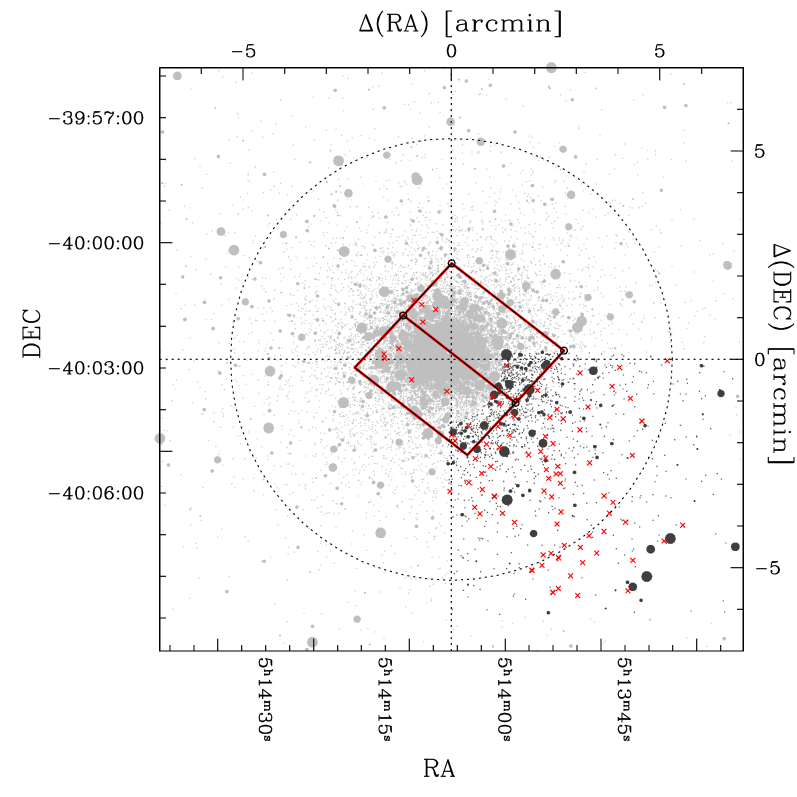
Figure 1: Area covered by the catalogs from which the spectroscopic selection was made: the FORS2 in the outer part (shown in black) and the ACS/HST field (continuous red line) in the inner region. The red crosses represent the IMACS+FORS2 sample. We also indicate the half tidal radius in this figure (dotted circle).

The resulting photometry was calibrated using stars in common with the $V,I$ Bellazzini et al. (2001) catalog, covering an 8’$\times$8’ field centered on the cluster. We also used publicly available Strömgren $u,v,b,y$ photometry of NGC 1851 from Grundahl et al. (1999) and Calamida et al. (2007). We refer the reader to that paper for details about observations and data reduction of Ströemgren photometry.

2.2 Observations and spectroscopic reductions

We acquired low-resolution (R$\simeq$1123 and R$\simeq$1246 at 3880 and 4305 Å, respectively) spectra of turnoff and SGB stars in the globular cluster NGC 1851 with the IMACS multi-object spectrograph at the Magellan 1 (Baade) telescope at the Las Campanas Observatory in Chile. The adopted instrumental setup with the grating GRAT 600-I covers the nominal spectral range between 3650-6750 Åwith a dispersion of 0.38Å /pix. This spectral range includes CN (3880 Å) and CH (4305 Å) molecular bands used to derive nitrogen and carbon abundances. However, the actual spectral coverage depends on the location of the slit on the mask with respect to the spectral dispersion. Because we observed faint stars, the total integration time was long, requiring ten exposures of 1800 sec each. Therefore all observations were made with a single-mask setup with 48 slits. We were able to extract spectra for 46 targets from our initial target list.

To these 46 spectra observed with Magellan, we added 47 other MS and SGB spectra from Pancino et al. (2010) observed with the FORS2 multi-object spectrograph on the ESO VLT at the Paranal Observatory in Chile. We refer the reader to that paper for details of the FORS2 observations. We reduced our data following the procedure described in Pancino et al. (2010). For the data pre-reduction, we used the standard procedure for overscan correction and bias-subtraction with the routines available in the noao.imred.ccdred package in IRAF. Cosmic rays were removed with the IRAF Laplacian edge-detection routine (van Dokkum 2001). The frames were then flat-fielded and reduced to one dimension spectra with the task apall. Once we obtained ten wavelength-calibrated, one-dimensional spectra for each star, we co-added them on a star-by-star basis to reach a relevant S/N (typically between 20-30 per pixel at 3880Å) even in the bluer part of the spectrum . As a final step, we examined each spectrum and rejected those spectra with bad quality, following the recipes outlined in Pancino et al. (2010). We defined several criteria for this rejection:

1. S/N ratio $<$ 10 (per pixel) in the CN 3880Å band;

2. clear defects (like spikes or holes) from an individual inspection of the spectrum on the band or continuum windows;

3. discrepant Ca(H+K) and $H_{\beta}$ index measurements.

Forty-three stars survived our criteria of selection. Moreover, 20 stars had spectral or continuum passbands falling in the gap between the CCDs because of the location of the slit on the mask with respect to the dispersion direction. We were not able to measure CH and CN band strengths for these stars, but in some cases we determined N and C abundances (Sect. 4). Therefore we decided to retain these spectra and consider them in the subsequent analysis.

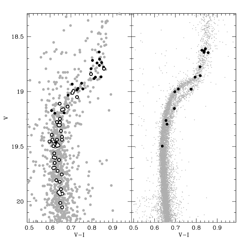
Figure 2: Color-magnitude diagrams for NGC 1851. Gray dots show $V-I$ photometry for the outer field (left panel) and inner field (right panel) from FORS2 and ACS, respectively. White dots mark spectroscopic targets presented in Pancino et al. (2010), while black dots show our newly observed stars.

2.3 Membership and quality control

NGC 1851 ($l,b=244.51,-35.08$; Harris 1996, 2010 edition) is projected at a far distance from the Galactic plane and consequently the contamination from field stars is almost negligible. In addition, the average radial velocity of cluster stars significantly differs with respect to the field (320.5 km/s; Harris 1996, 2010 edition), hence non cluster members can be easily identified from their radial velocities. For the stars in the ACS/WFC field of view, member stars were furthermore selected on the basis of their proper motions (see M08 for details).

For all the spectra, radial velocities were measured with the IRAF task fxcor, which performs the Fourier cross-correlation between the object spectrum and a template spectrum (the latter with known radial velocity). As a template we chose the spectrum of a star with the highest S/N: its radial velocity was computed using the laboratory positions of several strong lines (e. g. $H_{\beta}$, $H_{\alpha}$, $H_{\gamma}$ and $CaHK$ among others) with the IRAF task rvidlines. To derive a robust determination for the radial velocities, we performed for a given star the cross-correlation against the template in four different spectral regions that span the entire spectral coverage, from the bluest part out to the reddest part of the spectrum. Then, the four values were averaged together, obtaining typically internal errors of $\sim$ 25-30 $kms^{-1}$. We obtained an average $V_{rad}$ of 317 $kms^{-1}$ with a dispersion of 11 $kms^{-1}$, which fully agrees with the previous determination by Yong & Grundahl (2008), Villanova et al. (2010), and Carretta et al. (2010).

2.4 Additional literature data

To increase our observed sample, we added 47 MS and SGB stars observed with FORS2 that were presented by Pancino et al. (2010). The typical resolution of these spectra is R=$\lambda/\delta\lambda$$\simeq$800 and the S/N ratio (per pixel) in the CN band region is S/N(CN)$\simeq$30. More details concerning the observations and data reduction can be found in Pancino et al. (2010) and references therein. We reduced our data following the same procedure as adopted by these authors. Moreover, their definition of indices is exactly the same as ours (Sect. 3). While Pancino et al. (2010) did not need to normalize their spectra, this was necessary in our case, so we fitted a polynomial to the pseudo continuum to normalize both IMACS and FORS2 spectra as described in Sect. 3. We adopted the same procedure in determining the C and N abundance for both the newly obtained and previously studied spectra.

3 Index definition and measurements

Spectral indices are defined as a window centered on the molecular band of interest and one or two windows around it to define the continuum level. For each spectrum, S3839 and CH4300 indices sensitive to the absorption by the 3883Å CN band and the 4300Å CH band were measured. Several spectral index definitions exist in literature, generally optimized to quantify the CN content of the atmospheres of red giant stars. In our case, to be consistent with the previous work of Pancino et al. (2010), we decided to adopt the indices as defined in Harbeck et al. (2003):

$$S3839(CN)=-2.5\log\frac{F_{3861-3884}}{F_{3894-3910}}$$

$$S4142(CN)=-2.5\log\frac{F_{4120-4216}}{0.5F_{4055-4080}+0.5F_{4240-4280}}$$

$$CH4300=-2.5\log\frac{F_{4285-4315}}{0.5F_{4240-4280}+0.5F_{4390-4460}}.$$

In particular, the S3839(CN) index we used differs from that of Norris (1981) or Norris & Freeman (1979), and it accounts for stronger hydrogen lines in the region of CN feature for stars cooler than red giants. As an additional check, we defined and measured two different CN band indices in the wavelength region covered by our spectra: the S3839 for the CN band around 3880 Å and the S4142 for the one around 4200 Å. We obtained index measurement uncertainties with the expression derived by Vollmann & Eversberg (2006), assuming pure photon noise statistics in the flux measurements. In addition, we measured the two indices centered around the calcium H and K lines and the $H_{\beta}$ line as defined again in Pancino et al. (2010) to reject outliers from our sample.

The final reduced spectra generally show a strong decline of the signal toward bluer wavelengths. This is largely expected and may be due to the different instrumental efficiency, higher absorption of the Earth’s atmosphere in the blue and stellar flux wavelength dependency (see Cohen et al. 2002, for a complete discussion). The CH band at  4300 Å  is not affected by the change in spectral slope from atmosphere or instrumental effects thanks to two continuum bandpasses. On the other hand, we had to rely only on a single continuum bandpass in the red part of the spectral feature for the 3883Å CN band. Following Cohen et al. (2002, 2005), we decided to normalize the stellar continuum in the spectrum of each star, then found the absorption within the CN bandpass. Moreover, by fitting the continuum, we were able to directly compare the indices measured in this section and the abundances derived from spectral synthesis in Sect.4. We fitted a third-order polynomial masking out the region of the CN band (see Cohen et al. 2005). The polynomial fitting used a 6$\sigma$ high and 3$\sigma$ low clipping, running over a five pixel average. Then we computed S3839 indices from these continuum-normalized spectra and used the average (0.126$\pm$0.04 and 0.05$\pm$0.01 for IMACS and FORS2 spectra respectively) to set a zero point offset and thus delete the instrumental signature present in the raw S3839 indices.

The measured indices are listed in Tab. LABEL:indici_tab and plotted in Fig. 4.

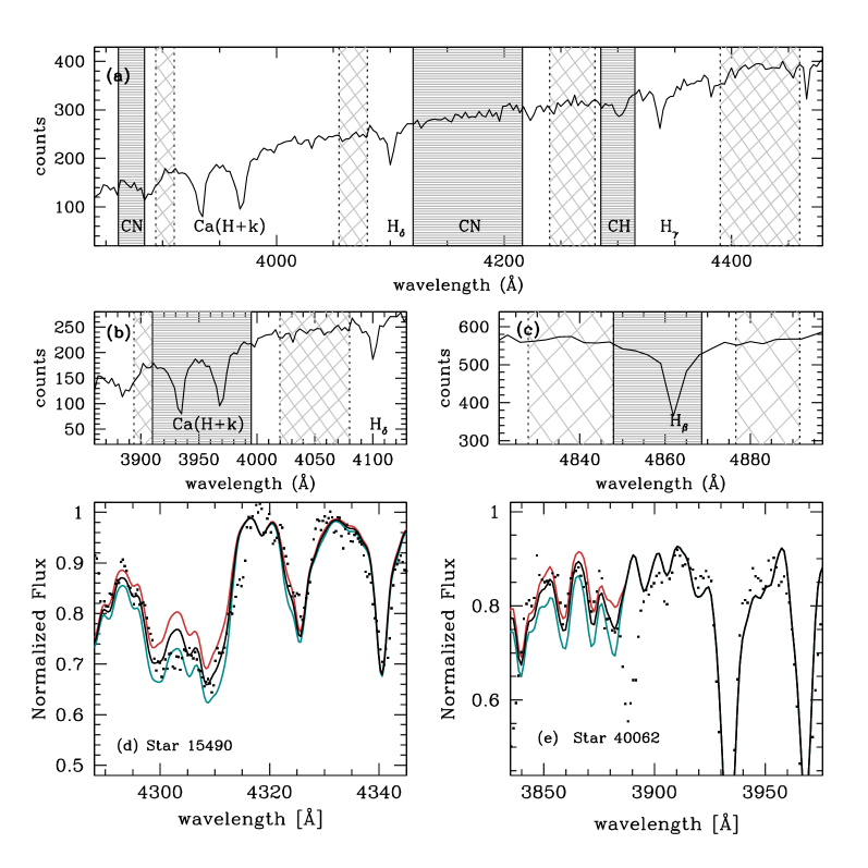
Figure 3: Panel a: example of the windows from which we measured the CN and CH indices (dark gray hatched regions) together with their respective continuum windows (light gray hatched regions). Panels b and c show the windows adopted for the H and K calcium index and the $H_{\beta}$ index. The non-normalized superimposed spectrum (star 41213, S/N$\sim$35 in the S3839 region) was smoothed for clarity. Panel d: Observed (small black dots) and synthetic (line) spectra around CH band for the star 15490. The black best fits, while the red and green lines are the syntheses computed with C abundance altered by $\pm$ 0.10 dex from the best value. Panel e: The same as in panel d but for the CN feature for the star 40062. The synthetic spectra show the best fit (thick black line) and the syntheses computed with N abundance altered by $\pm$ 0.20 (thick red and green lines).

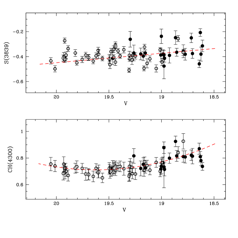
Figure 4: Measured S3839 and CH4300 indices for the program stars as a function of $V$. White dots are stars from Pancino et al. (2010), while black dots are from the IMACS sample. Dashed red lines in both panels are the median ridge lines used to eliminate temperature and gravity dependencies.

3.1 Dependency on temperature and gravity

CN and CH bands are stronger at a fixed overall abundance for stars with lower temperature and gravity. In particular, the formation efficiency of the CN molecule strongly depends on the temperature, therefore we expect the indices depend on the color of the single stars. These dependencies are usually eliminated (see Harbeck et al. 2003; Kayser et al. 2008, for example) by fitting the lower envelope of the distribution in the index-magnitude plane (or index-color plane). For our sample, we used the median ridge line, shown as dashed red lines in Fig. 4, to eliminate these dependencies (see Pancino et al. 2010). These rectified CN and CH indices are in the following indicated as $\delta$S3839 and $\delta$CH4300, respectively, and we refer to these new indices throughout. For the stars in common between this work and Pancino et al. (2010), the mean difference in the $\delta$S3839 and $\delta$CH4300 indices, derived by subtracting Pancino et al.’s values from ours, are 0.00 $\pm$ 0.02 mag and –0.01$\pm$0.01 mag, respectively. Because we adopted the same reduction procedures as in Pancino et al. (2010), we can only ascribe this small difference to the continuum normalization we performed (see Sect. 3).

3.2 CN and CH distribution

Variations of several light elements and anticorrelations between strengths of the CN and CH bands were detected for very many clusters. Because molecular abundance is controlled by the abundance of the minority species, the corrected CH index is a proxy for carbon abundance, while $\delta$S3839 traces the nitrogen abundance. The visual inspection of the top panel of Fig. 4 reveals significant scatter in the CN index over the magnitude range with $V\gtrsim$ 19.5 with some hints of bimodality toward the brightest tail of the distribution. The range of CN becomes less evident at fainter luminosities as a consequence of the increasing temperature. In the bottom panel of the same figure, we plot the CH4300 and S3839 versus the stellar V-band magnitudes. Here the variations among the measured index are very small and within the uncertainties throughout.

Figure 5 shows the rectified index $\delta$S3839 as a function of $\delta$CH4300 for all stars. We found no evidence for a significant CH-CN anticorrelation, similarly to what was found by Pancino et al. (2010).

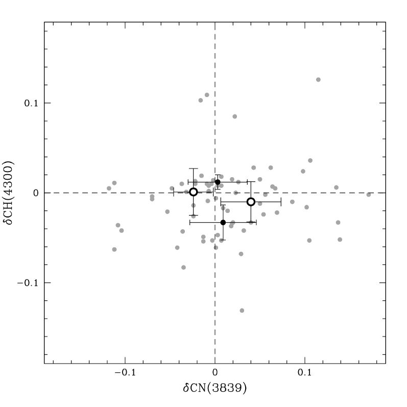
Figure 5: Plot for the distribution of CN and CH band strengths. Gray dots show measurements for stars. CH-weak and CH-strong stars are separated by the horizontal dashed line and their centroids with error bars (drawn at 1$\sigma$) are marked as black dots and large empty dots, respectively.

4 Spectral synthesis and abundance derivations

Indices are a fast tool to characterize chemical anomalies, but we can also rely on spectral synthesis to fully characterize our target stars. This becomes necessary when indices do not offer conclusive answers, as we saw in the previous sections.

4.1 Atmospheric parameters

We derived estimates of the atmospheric parameters from the calibrated ACS and FORS2 photometry presented in Sect. 2. Dereddened $(V-I)_{0}$ colors were obtained adopting $E(B-V)$ = 0.02 (Harris 1996, 2010 edition). We obtained effective temperatures and bolometric corrections (hereafter $T_{eff}$ and $BC_{V}$) with the Alonso et al. (1996, 1999, 2001) color-temperature relations, adopting [Fe/H]= -1.22 from Yong et al. (2009), and taking into account the uncertainties in the magnitudes and reddening estimates. Alonso et al. (1996, 1999) adopted Johnson’s system as a reference, therefore we converted $(V-I_{C})$ into $(V-I_{J})$ after dereddening using the prescriptions by Bessell (1979) to feed the Alonso et al. (1996, 1999, 2001) calibration. Gravities were then obtained by means of the fundamental relations

$$\log\frac{g}{g_{\sun}}=\log\frac{M}{M_{\sun}}+2\log\frac{R_{\sun}}{R},$$

$$0.4\leavevmode\nobreak\ (M_{bol}-M_{bol,\sun})=-4\log\frac{T_{eff}}{T_{eff,\sun}}+2\log\frac{R_{\sun}}{R},$$

where we assumed the solar values reported in Andersen (1999): $\log{g_{\sun}}$ = 4.437, $T_{eff,\sun}$ = 5770K and $M_{bol,\sun}$ = 4.75. For all our stars, we assumed a typical mass of 0.8 $M_{\sun}$ (Bergbusch & VandenBerg 2001) and a distance modulus of $(m-M)_{V}$ = 15.47 (Harris 1996, 2010 edition).

Finally, we obtained the microturbulent velocities ($v_{t}$) from the relation $\log g$ and $v_{t}$, i.e., $v_{t}=1.5-0.03\log g$ as in Carretta et al. (2004). This method leads to an average microturbulent velocity estimate of $v_{t}=1.0\pm 0.1$ km$s^{-1}$, therefore we assumed $v_{t}=1.0$ km $s^{-1}$ for the entire sample. An additional check to test the reliability of our atmospheric parameter determination was performed using theoretical isochrones downloaded from the BaSTI database (Pietrinferni et al. 2006). We chose an isochrone of 11 Gyr (12 Gyr for the faint-SGB) with standard $\alpha$-enhanced composition, and metallicity Z = 0.002 and we projected our targets on the isochrone to obtain their parameters. We present the average difference between the two methods in Fig. 6. In the top panel we plot the difference in temperature obtained using the Alonso et al. (1999) calibration and the temperature obtained by projection of the star on the BaSTI isochrones as a function of the temperature derived by means of the Alonso et al. (1999) empirical relations. The scatter for high temperatures is significant, as largely expected, because these empirical calibrations were obtained for giant stars and therefore are valid in a precise range of color. On the other hand, the scatter is modest (and in many cases within uncertainties) when comparing temperatures obtained by using theAlonso et al. (1999) and Alonso et al. (1996) relations (see bottom panel of Fig. 6), where the latter was derived for low main sequence stars. However, we preferred to avoid using temperatures derived by isochrone fitting mainly for these reasons: (a) we cannot assume a priori that the cluster is a single population (with the same [Fe/H] and CNO content, among others) and (b) the projection on the ($V,V-I$) plane is always uncertain, and a rigorous treatment should include (asymmetrical) errors on the $V$ magnitude and $V-I$ color, and finally, (c) different sets of isochrones (Padova, BaSTI, and DSEP for example) give different results.

Figure 6: Top panel: Differences in the temperature estimates by means of isochrone projection procedure and using the Alonso et al. (1999) relation ($\Delta(T_{iso}-T_{A99}$)) as a function of the Alonso et al. (1999) temperature ($T_{A99}$) for all our target stars. Bottom panel: The same, but for the Alonso et al. (1996) calibration ($T_{A96}$).

As discussed in the following sections, even if the differences between the two temperatures scales appear non-negligible, the main results of the paper appear totally unchanged if we adopt one or the other temperature scale. This is mainly because the abundances ranking among target stars is left unchanged. We therefore preferred to rely on the Alonso et al. (1999) parameter estimates and discuss the effect of the chosen temperature scale below.

4.2 Abundances derivation

We used the local thermodynamic equilibrium (LTE) program MOOG (Sneden 1973) combined with the ATLAS9 model atmospheres (Kurucz 1993, 2005) to determine carbon and nitrogen abundances. The atomic and molecular line lists were taken from the latest Kurucz compilation and downloaded from F. Castelli’s website.

Model atmospheres were calculated with the ATLAS9 code starting from the grid of models available in F. Castelli’s website, using the values of $T_{eff}$, $\log g$, and $v_{t}$ determined as explained in the previous section. The ATLAS9 models employed were computed with the new set of opacity distribution functions (Castelli & Kurucz 2003) and excluding approximate overshooting in calculating the convective flux. For the CH transitions, the $\log$ g obtained from the Kurucz database were revised downward by 0.3 dex to better reproduce the solar-flux spectrum by Neckel & Labs (1984) with the C abundance by Caffau et al. (2011), as extensively discussed in Mucciarelli et al. (2011).

C and N abundances were estimated by spectral synthesis of the 2$\Sigma$–2$\Pi$ band of CH (the G band) at $\sim$4310Å and the $UV$ CN band at 3883Å (including a number of CN features in the wavelength range of 3876-3890Å), respectively. Lower panels of Fig. 3 illustrate the fit of synthetic spectra to the observed ones in CH and CN spectral regions. Abundances for C and N were determined together in an iteractive way, because for the temperature of our stars, carbon and nitrogen form molecules and as a consequence their abundances are related to each other. The input model atmosphere was used within the MOOG running synth driver that computes a set of trial synthetic spectra at higher resolution (0.3Å intervals) in the spectral region between 4150-4450Å, varying the carbon abundance in steps of 0.1 dex typically in the range of –0.2 to –1.2 dex to fit a full band profile. After the synthesis computations, the generated spectra were convolved with Gaussians of appropriate FWHM to match the resolution of the observed spectra. In this way, the carbon abundances were derived by minimizing the observed-computed spectrum difference and were used to determine A(C). The carbon abundance was then used as input in the synthesis of the $UV$ CN feature to derive nitrogen abundances. The procedure was repeated until we obtained convergence within a tolerance of 0.1 dex in the C and N abundances.

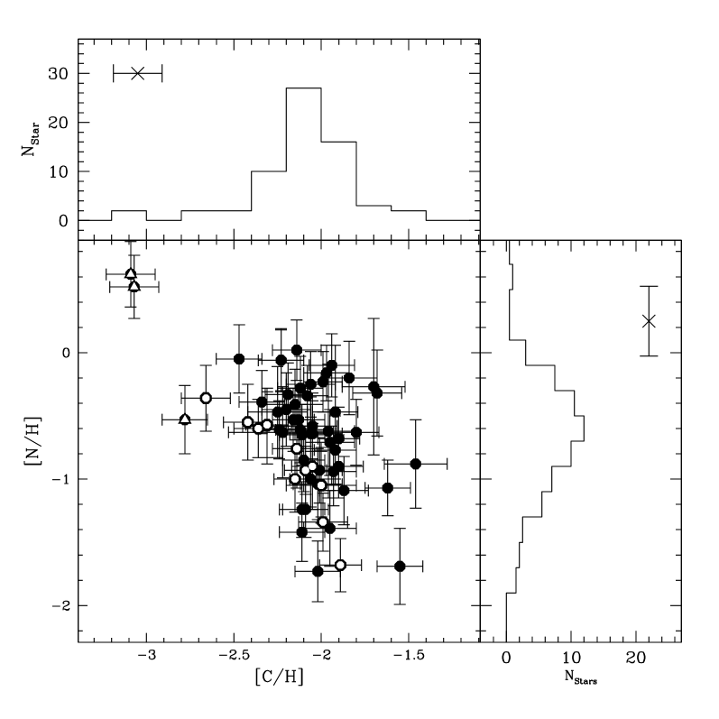
Figure 7: [C/H] and [N/H] abundances for the NGC1851 SGB, TO and MS stars in Table LABEL:stellar-par1 are plotted. A C versus N anticorrelation is evident. Stars that have already experienced some mixing episode are shown as large white dots, while three notable outliers are represented as large triangles (see text for comments). Histograms of [N/H] and [C/H] with typical median error bars are also plotted in this figure.

For the results presented here, a fit was determined by minimizing the observed-computed spectrum difference in a 60Å window centered on 4300Å for the CH $G$-band and 40Å window for the $UV$ CN feature at 3883Å. Running synth on quite a broad spectral range (200 and 300Å for the $G$-band and the CN feature, respectively) to produce synthetic spectra allowed us to set a reasonable continuum level also by visual inspection and thus compute robust abundances.

We adopted a constant oxygen abundance ([O/Fe]=0.4 dex) throughout all computations. The derived C abundance is dependent on the O abundance and therefore so is the N abundance, and in molecular equilibrium an over-estimate in oxygen produces an over-estimate of carbon (and vice versa), and an over-estimate of carbon from CN features is refleced in an under-estimate of nitrogen. We expect that the exact O values will affect the derived C abundances only negligibly, since the CO coupling is marginal for stars warmer than $\sim$ 4500 K. To test the sensitivity of the C abundance to the adopted O abundance we varied the oxygen abundances and repeated the spectrum synthesis to determine the exact dependence for a few representative stars in a wide range of $T_{eff}$ (from 5200 to 5900 K). In these computations, we adopted [O/Fe]= -0.5 dex, [O/Fe]= 0.0 dex, [O/Fe]= +0.5 dex. We found that strong variations in the oxygen abundance slightly affect ($\delta A(C)/\delta[O/Fe]\simeq$ 0.15 dex) the derived C abundance in colder stars ($T_{eff}$$\leq$ 5400 K), while they are completely negligible (on the order of 0.05 dex or less) for warmer stars. This is within the uncertainty assigned to our measurement.

The total error in the A(C) and A(N) abundance was computed by taking into account the two main sources of uncertainty: (i) the error in the adopted $T_{eff}$, typically $\delta$A(C)/$\delta T_{eff}\simeq$ 0.08–0.10 dex and $\delta$A(N)/$\delta T_{eff}\simeq$ 0.11–0.13 per 100 K for the warmest stars in our sample; (ii) the error in the fitting procedure and errors in the abundances that are likely caused by noise in the spectra. The errors due to uncertainties on gravity and microturbulent velocity are negligible (on the order of 0.02 dex or less). The sensitivity of the derived abundances to the adopted atmospheric parameters was obtained by repeating our abundance analysis and changing only one parameter at each iteration for several stars that are representative of the temperature and gravity range explored. Thus, we assigned the internal error to each star depending on its $T_{eff}$ and $\log g$. The errors derived from the fitting procedure were then added in quadrature to the errors introduced by atmospheric parameters, resulting in an overall error of $\sim\pm$0.14 dex for the C abundances and $\sim\pm$0.28 dex for the N values.

Very recently Carretta et al. (2010) found in NGC 1851 a small spread in metallicity for a large number of giants, which is compatible with the presence of two different groups of stars whose metallicity differs by 0.06-0.08 dex (but this result was not confirmed in Villanova et al. 2010) . This finding could affect our analysis in principle, because we adopted the same metallicity for all our stars in the synthesis ([Fe/H]=-1.22). To test this effect we repeated the synthesis by altering the metallicity of stars belonging to the faintest SGB by 0.10 dex (well above the spread claimed by Carretta et al. 2010). The resulting abundance variations are within the uncertainty assigned to our measurement (typically $\delta A(C)/\delta[Fe/H]\simeq$ 0.07 dex and $\delta A(N)/\delta[Fe/H]\simeq$ 0.04 dex) for our low-resolution spectra. Therefore this potential small [Fe/H] variation among our spectroscopic targets has no influence on our analysis and conclusions. We present the abundances derived as described above and the relative uncertainties in the abundance determination in Tab. LABEL:stellar-par1. Additionally, this table lists the derived atmospheric parameters of all our targets.

4.3 C and N abundance results

Fig. 7 plots [C/H] versus [N/H] measured in this paper. We observe strong star-to-star variations in both elements, as already observed in all GCs studied to date. An anticorrelation, with considerable scatter, is apparent from Fig. 7. The scatter is consistent with the observational errors, but there are a few outliers. In a sample of 64 objects with Gaussian errors, two outliers at the 3 $\sigma$ level are not expected. The deviation of stars 41350 (V = 19.3) and 40022 (V=19.9) with extremely depleted C, from the mean relation shown by the NGC 1851 sample in Fig.7 is of higher statistical significance. We cannot provide a reliable explanation for this. Both stars are from the Pancino et al. (2010) sample and, judging from their radial velocities, are cluster members. Moreover, their $V,I$ magnitudes do not have large errors. As a tentative hypothesis we suggest that these two stars could belong to the extreme population, using the scheme suggested by Carretta et al. (2009).

All our stars are C-depleted, with moderately weak variations in carbon abundances (from [C/H]$\sim$–2.7 to [C/H]$\sim$–1.5) anticorrelated with strong variations in N. The nitrogen abundance spans almost 2 dex, from [N/H]$\sim$–1.9 up to [N/H]$\sim$0.0 dex. To check the dependence of the carbon and nitrogen abundances on the adopted temperature scale, we re-ran the synthesis using the atmospheric parameters derived by isochrone fitting (see Sect. 4.1). The result of this exercise is shown in Fig. 8. As can be seen from this figure, the carbon abundances would be higher considering these higher temperatures (ranging from $\sim$ 0.2 dex for giants up to 0.4-0.5 dex for Ms stars). This reflects on the nitrogen abundances, as demonstrated in the bottom panel of the same figure. This is only to show that the abundances ranking among target stars is left unchanged: while the zero point of our derived abundances would shift, the amplitude of the star-to-star variations for C and N would remain similar regardless of the adopted stellar parameter. Therefore, our conclusions do not depend on the adopted stellar parameters.

Figure 8: Comparison of carbon (top) and nitrogen (bottom panel) abundances derived by adopting different temperature scales (”A99” refers to the Alonso et al. 1999 calibration and ”iso” to the isochrones fitting procedures) with their relative uncertainties.

Evaluating the accuracy of our absolute abundance scale is very difficult because we found no literature data to compare with. Fig. 9 compares the C and N abundances of this paper to the abundances derived for M 5 by Cohen et al. (2002), a cluster with a metallicity comparable ($\sim$–1.29; Harris 1996, 2010 edition) to that of NGC 1851. In panel (a) we present a comparison between C and N abundances derived by assuming the Alonso et al. (1999) temperature scale and abundances derived by Cohen et al. (2002) for stars at the base of the RGB in M 5, while panel (b) refers to isochrones-fitting temperatures. In both panel a clear C-N anticorrelation is apparent. According to theoretical computations and earlier investigations, the carbon abundance declines from MS to RGB. In panel (a) there is a mild disagreement with the Cohen et al. (2002) data; that is completely reconciled in panel (b). This effect can be entirely explained because Cohen et al. (2002) used atmosphere parameters obtained from the isochrone. Still, although there is an offset, the two anticorrelations seem to follow a similar pattern. We conclude again from Fig. 9 that the anticorrelation we observe is totally untouched by the choice of the temperature scale, and shifts in the absolute abundance scale cannot account for the wide range in N abundances apparent in Fig.7.

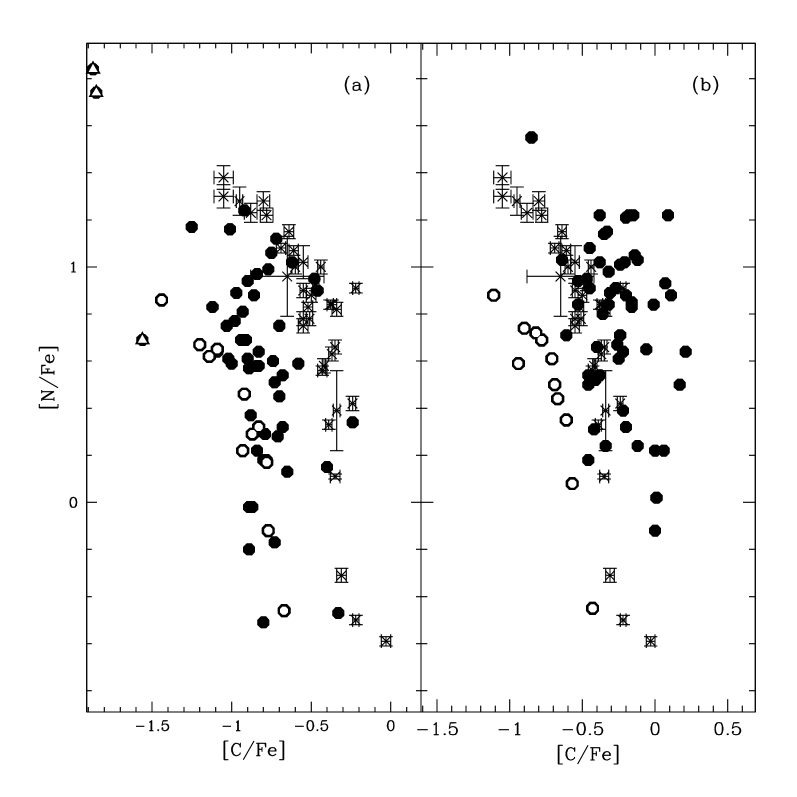
Figure 9: Panel (a): [C/Fe] and [N/Fe] abundances for NGC 1851 stars. Stellar atmospheres and spectral syntheses were derived by assuming the Alonso et al. (1999) temperature scale. The symbols are the same as in Fig. 7. Abundances and relative uncertainties for stars in M 5 from Cohen et al. (2002) are also shown as crosses for comparison. Panel (b): the same as in the left panel, but assuming temperatures and gravities obtained from the isochrones.

We therefore conclude that the C versus N anticorrelation among unevolved NGC 1851 stars in Fig.7 is indeed real and from here on we will therefore only present results based on the Alonso et al. (1999) temperature scale.

We also plotted the derived abundances as a function of the $V$ magnitude and $V-I$ color in Fig. 10 to evaluate possible systematic effects with luminosity and temperature.

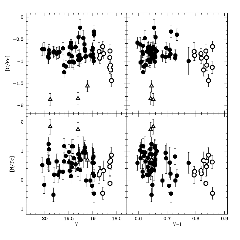
Figure 10: Derived C and N abundances are plotted against the photometry for NGC 1851 stars. No systematic trends with either luminosity or temperature are apparent in the abundances. We call stars marked as black empty triangles anomalous, while stars that supposedly underwent some mixing episodes are plotted as empty dots (see text).

While none of these effects are apparent, we can tentatively identify the occurrence of a mixing episode for NGC 1851 stars from this plot. The top panel of Fig. 10 shows a notable decline in the carbon abundances for stars with $V\lesssim$18.9 and $(V-I)\gtrsim$0.8 (stars marked as white dots in the same figure), which is expected for stars in the course of normal stellar evolution. This behavior of the C abundance allows us to identify stars that experienced a major mixing episode, which may alter the primordial abundances. Curiously enough, these stars, plotted again as large white dots, seem to define a pretty clear and narrow anticorrelation in Fig.7 (Spearman’s rank correlation coefficient –0.92). The shape of this anticorrelation agrees with what we expect after the occurrence of a mixing episode: the high N enhancement found in unevolved or less-evolved stars is strongly softened by evolutionary effects and a large part of dwarfs and early subgiants have N abundances as high as those observed in slightly evolved RGB stars. We identify, again from Fig. 10, three outliers, coded as empty triangles as in Fig. 7. Two of these stars were found to deviate significantly from the main C-N relation if Fig. 7. We call these anomalous only by virtue of their positions in the upper panel of Fig. 10 and decided to not consider them further.

At this point we note that we cannot arbitrarily distinguish between two groups of stars with different [N/H] or [C/H] because we are unable to detect any clear bimodality. To be more quantitative, we ran the dip test on unimodality (Hartigan & Hartigan 1985). We performed this simple statistical test only on stars with a magnitude $V<$18.9 and can confirm that there is no bimodality in either the [C/H] or [N/H].

Figure 11: CMD for NGC 1851 from Strömgren photometry. The inset shows a zoom of the SGB region. Only stars with high-quality photometry were plotted (see Sect. 5.1 for details). Note the discrete double RGBs connected with the bimodal SGBs.

5 The chemical composition of the double RGB and SGB

As already discussed in Sect. 1, the discovery of multiple sequences in the CMD of NGC 1851 provided unambiguous proof of the presence of multiple populations and brought new interest and excitement about this GC. While it is now widely accepted that NGC 1851 hosts two or more stellar populations, the connection among its multiple SGBs, RGBs, and HBs is still controversial and the chemical composition of the two SGBs is also debated.

Figure 12: Main panel: Reproduction of the CMD of Fig. 11. We used red color codes for red-RGB and faint-SGB stars, while blue-RGB and bright-SGB stars are represented in blue. Symbols refer to stars from spectroscopic studies as indicated in the figure. The rectified CMD and the histogram color distribution of RGB stars between the two dashed lines is shown in the inset (see text for details).

Several authors suggested that the groups of $s$-rich and $s$-poor stars detected from RGB-star spectroscopy are the progeny of the faint- and bright-SGB, respectively (e. g. M08, Yong & Grundahl 2008), in close analogy to what was observed in M22 and $\omega$ Centauri (e. g. Marino et al. 2009, 2011; Johnson & Pilachowski 2010; Pancino et al. 2011). In contrast, Carretta et al. (2011) claimed that the faint-SGB consists of barium-poor metal-poor stars while bright-SGB stars have an enhanced barium and iron abundance.

5.1 Photometric connection between SGB and RGB

To investigate this question in more detail, we started analyzing literature photometry. We used the WFC/ACS HST CMD in F606W and F814W bands presented in M08 (see Sarajedini et al. 2007; Anderson et al. 2008, for details) and the Strömgren $u$, $b$, $v$, $y$ photometry from Grundahl et al. (1999) and Calamida et al. (2007). Here we are interested in high-quality photometry and included in the analysis only relatively isolated, unsaturated stars with good values of the PSF-quality fits and small rms errors in astrometry and photometry. A detailed description of the selection procedures is given in Milone et al. (2009, Sect. 2.1). We corrected our photometry for remaining spatially dependent errors, caused by small inaccuracies of the PSF model (see Anderson et al. 2008). To account for the color differences of these variations we followed the recipes from Milone et al. (2011, Sect. 3). Briefly, we defined a fiducial line for the MS by computing a spline through the median colors found in successive short intervals of magnitude, and we iterated this step with a sigma clipping; then we examined the color residuals relative to the fiducial and estimate for each star, how the observed stars in its vicinity may systematically lie to the red or the blue of the fiducial sequence. Finally we corrected the star’s color by the difference between its color residuals.

To study multiple populations from the CMD analysis, we started searching for the combination of magnitude and colors that provides the best separation of the two RGBs and SGBs in NGC 1851. Results are illustrated in Fig. 11 where we plot $u$ as a function of ($u-y$)$+$($v-b$). A visual inspection of this diagram leaves no doubts on the presence of a bimodal RGB and SGB and shows that the faint-SGB and the bright-SGB are clearly connected with the red- and the blue-RGB, respectively. A similar connection between the two SGBs and RGBs has already been observed for NGC 1851 by Han et al. (2009) in the $U$ versus ($U-I$) CMD and was studied more recently by Sbordone et al. (2011). These authors showed that while the double SGB is consistent with two groups of stars with either an age difference of about one Gyr or with different C+N+O overall abundance, the double RGB seems to rule out the possibility of a large age difference.

Fig. 11 revealed that the bimodality found in the SGB can also be seen in the RGB. To further confirm our association of the faint-SGB (bright-SGB) component with the red-RGB (blue-RGB), we focused on the relative number of stars of all evolutionary stages. To estimate the fraction of stars in the two RGBs we used only RGB stars between the two dashed lines in the magnitude interval where the split is more evident (main panel of Fig. 12). The procedure is illustrated in the inset of Fig. 12. To obtain the straightened RGB of the right-hand panel, we subtracted from the color of each star the color of the fiducial sequence at the $u$ magnitude of the star. The color distribution of the points in the middle panel were analyzed in two magnitude bins. The distributions have two clear peaks, which we fitted with two Gaussians (red for the red-RGB and blue for the blue-RGB). From the areas below the Gaussians, 70$\pm$3% of stars turn out to belong to the blue-RGB, and 30$\pm$3% to the red one. With the statistical uncertainties these fractions are the same in both magnitude intervals and roughly match the relative frequency on the fainter/brighter SGBs (35% versus 65%, M08) and HB stars on the blue/red side of the instability strip (35% versus  65%).

Table 3: Mean abundances for NGC 1851 stars from high-resolution studies.

Element	Abundance (blue-RGB)	$N_{\rm stars}$	Abundance (red-RGB)	$N_{\rm stars}$	References
$[$La/Fe$]$	0.27$\pm$0.02	5	0.61$\pm$0.05	3	1
$[$Na/Fe$]$	–0.05$\pm$0.11	5	0.57$\pm$0.15	3	1
$[$O/Fe$]$	0.50$\pm$0.04	5	0.17$\pm$0.14	3	1
$[$Fe/H$]$	–1.29$\pm$0.04	5	–1.23$\pm$0.07	3	1
$[$Ba/Fe$]$	0.09$\pm$0.02	8	0.52$\pm$0.03	7	2
$[$Na/Fe$]$	0.04$\pm$0.11	8	0.47$\pm$0.07	7	2
$[$O/Fe$]$	0.09$\pm$0.07	8	–0.19$\pm$0.08	7	2
$[$Fe/H$]$	–1.23$\pm$0.01	8	–1.22$\pm$0.01	7	2
$[$Ba/Fe$]$	0.43$\pm$0.02	72	0.78$\pm$0.04	21	3
$[$Na/Fe$]$	0.13$\pm$0.03	81	0.47$\pm$0.04	24	3
$[$O/Fe$]$	0.04$\pm$0.02	66	–0.14$\pm$0.05	17	3
$[$Fe/H$]$	–1.16$\pm$0.01	82	–1.15$\pm$0.01	24	3
$[$Ba/Fe$]$	0.51$\pm$0.04	8	0.94$\pm$0.09	3	3
$[$Na/Fe$]$	0.20$\pm$0.07	8	0.57$\pm$0.11	3	3
$[$O/Fe$]$	0.12$\pm$0.08	8	–0.27$\pm$0.13	3	3
$[$Fe/H$]$	–1.18$\pm$0.01	8	–1.14$\pm$0.08	3	3

(1) Yong & Grundahl (2008); (2) Villanova et al. (2010); (3) Carretta et al. (2011).

5.2 Chemical composition of NGC 1851 subpopulations

Because the chemical abundance determinations presented so far do not define any clear bimodality, the clear separation of the sequences of Fig. 11 provides a unique opportunity to obtain information on the chemical differences between the two RGBs and SGBs in NGC 1851. To do this, we used a $u,(u-y)+(v-b)$ diagram to isolate the samples of blue-RGB and bright-SGB stars, and red-RGB and faint-SGB stars. Then we plotted with red and blue symbols the red-RGB and blue-RGB stars for which abundance measurements are available from high-resolution spectroscopy.

Figure 13: Upper panel: Na-O anticorrelation among NGC 1851 RGB stars from HR spectroscopy studies. Red color refers to stars photometrically selected to belong to the red-RGB in the Strömgren $u$, $(u-y)+(v-b)$ diagram, while stars located on the blue-RGB are shown in blue. Symbols and color code are consistent with those of Fig. 12. Bottom panel: The run of [La/Fe] versus [Fe/H] and the normalized number distribution for red and blue stars in this plane. The color code is consistent with the upper panel.

Figure 14: Left panel: selected bright-SGB (marked as blue dots) and faint-SGB (shown as red squares) stars are overplotted on the $V,V-I$ CMD presented by M08. Right panel: selected bright- and faint-SGB stars are shown in the Strömgren $u$, $(u-y)+(v-b)$ diagram. The color code is consistent with the left panel.

Our analysis of the chemical abundance patterns of the two RGBs is summarized in Fig. 13. Lower panels show [Fe/H] versus the abundances of the $s$-process elements barium and lanthanum measured by Yong & Grundahl (2008), Villanova et al. (2010), and Carretta et al. (2011) from GIRAFFE and UVES data. The histogram of the $s$-element distribution is illustrated in the middle panel, while upper panels plot [Na/Fe] versus [O/Fe]. The average iron, barium, lanthanum, sodium, and oxygen abundances are listed in Table 3 for the two groups of stars.

Figure 15: Photometrically selected bright-SGB (marked as blue dots) and faint-SGB (shown as red squares) stars are represented in the A(C) versus A(N) plane. Stars that we were unable to unambiguously associate with either of the two populations are shown with open circles.

In the light of our analysis of literature photometric and spectroscopic data we are now able to characterize the two RGBs and SGBs of NGC 1851 as follows:

• Faint-SGB and red-RGB stars are photometrically connected, therefore they represent the same subpopulation of NGC 1851; the same can be said about bright-SGB and blue-RGB (see also Marino et al. 2012b, for the case of M 22). This connection is supported by the relative (percentage) numbers of the sequences; therefore the data do not support the interpretation by Carretta et al. (2010) that the red-RGB is associated to the bright-SGB.

• Literature data suggest that the red-RGB stars tend to be enriched on average in Na and $s$-process elements, and poor in oxygen, while blue-RGB stars appear to have their own, extended anticorrelation and to be solar in Ba and $s$-process elements. This is particularly evident in the Carretta et al. (2011) dataset, which also has the highest statistical value.

• Red-RGB (and thus faint-SGB, according to our interpretation above) stars are enhanced in barium and lanthanum by $\sim$0.3-0.4 dex with respect to the blue-RGB (and consequently the bright-SGB).

• The literature data suggest that there is no significant iron difference between the two groups of stars. In this context we recall that Yong & Grundahl (2008) and Carretta et al. (2011) detected a significant [Fe/H] variation among both $s$-rich and $s$-poor stars but these results strictly disagree with the narrow iron distribution observed by Villanova and collaborators. The presence of an intrinsic iron spread among NGC 1851 stars is still controversial.

5.3 C and N abundances along the double SGB

In this section we present the chemical composition of stars on the two SGBs of NGC 1851. A bona fide sample of stars that belong unambiguously either to the faint-SGB or to the bright-SGB were selected using both the $V$, $V-I$ and $u$, $(u-y)+(v-b)$ diagrams (see Fig. 14).

The C and N abundances of these bona fide stars are plotted in Fig. 15, where it is immediately clear that stars belonging to the bright-SGB show a fully developed anticorrelation, while stars belonging to the faint-SGB appear to have a smaller scatter, and to have on average an excess of N (this remains still valid when considering temperatures derived by isochrone fitting as input of the synthesis, as anticipated in Sect. 4.3). This new result supports our previous identification of the faint-SGB as the parent population of the red-RGB, and of the bright-SGB as the parent of the blue-RGB, not only on the basis of photometry and population ratios, but also on the basis of chemical composition.

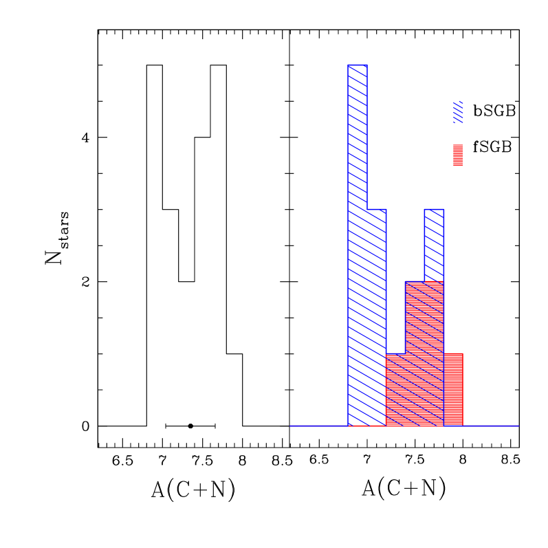
Figure 16: Left panel: Histogram of the C+N distribution for SGB stars selected as described in Sect. 5.3. The median error bar is plotted below the histogram for reference. Right panel: Histograms of the C+N sum for bright-SGB (dashed blue) stars and faint-SGB (hatched red) stars are shown.

Cassisi et al. (2008) and Ventura et al. (2009) argued that the overall CNO abundance difference can account for the SGB split. Yong et al. (2009) found evidence for strong CNO variations in contradiction with the the results of Villanova et al. (2010). To further investigate this hypothesis, we computed the C+N sum for our bona fide faint-SGB and bright-SGB stars. We then derived the histograms of the distribution of the C+N sum. In the left panel of Fig. 16, we plot the histograms for the entire dataset (faint-SGB + bright-SGB bona fide stars) with the typical (median) error bar indicated. The histogram shows a high dispersion with a hint of bimodality (with two clumps separated at A(C+N)$\simeq$7.35). For this larger dataset, according to a KMM test (Ashman et al. 1994), a bimodal distribution is a statistically significant improvement over the single Gaussian at a confidence level of 89%. However, a much clearer result is obtained when histograms are built considering the bright- and the faint-SGBs separately (right panel of Fig. 16): they have a different (averaged) C+N content, the faint-SGB having A(C+N)$\simeq$7.64$\pm$0.24 and the bright-SGB A(C+N)$\simeq$7.23$\pm$0.3 (A(C+N)$\simeq$7.80$\pm$0.19 and A(C+N)$\simeq$7.47$\pm$0.26; using isochrone fitting temperatures, respectively, see Sect. 4.3). As an additional check, we performed a two-sample KS test computing the probability that these two samples are drawn from the same parent distribution and found a pretty high ($P_{KS}$ $\sim$0.03) significance of the difference in the bright-SGB and faint-SGB distribution of A(C+N). From Fig. 15 bright-SGB stars appear to be on average more N-poor than then faint-SGB stars; assuming an N-O anticorrelation, the bright-SGB stars are more O-rich than the faint-SGB stars. Even though we do not provide oxygen abundances for our SGB stars, we can speculate on the C+N+O sum for the two SGB components assuming [O/Fe] values from available measurements. Various oxygen abundance determinations of RGB stars can be found in the literature. From Fig. 13 we just note that large systematic differences exist between different determinations of the O content (see also Tab. 3) and we caution readers that assigning a reference [O/Fe] content to each SGB group could be naïve at this stage. If we assume for the bright and faint component [O/Fe]$\simeq$0.1 dex and [O/Fe]$\simeq$–0.2 dex, respectively, the separation one sees in C+N content virtually disappears when considering C+N+O. We found that the faint-SGB have A(C+N)$\simeq$7.89$\pm$0.14 and the bright-SGB A(C+N)$\simeq$7.93$\pm$0.07. The distributions even swap when considering O abundances suggested by Yong & Grundahl (2008) ([O/Fe]$\simeq$0.5 dex and [O/Fe]$\simeq$0.2 dex for the bright- and faint-SGB stars, respectively. We conclude that the bimodality we observe in the C+N sum does not necessarily imply or exclude a bimodality in the C+N+O content and more observations are needed to settle the case of NGC 1851.

6 Summary and discussion

We presented low-resolution spectroscopy for a large sample of MS and SGB stars in NGC 1851 with the goal of deriving C abundances (from the G band of CH) and N abundances (from the CN band at $\sim$ 3883Å) and investigating the chemical differences between the two branches of the double SGB. We derived carbon and nitrogen abundances for 64 stars, whose spectra were obtained with FORS2 at VLT and IMACS at Magellan and analyzed in a uniform manner.

NGC 1851 is one of the most interesting GCs whose CMD displays a discrete structure at the level of the SGB and of the RGB. The photometric complexity is reflected in a peculiar chemical pattern that has only recently been investigated in detail. So far, the available abundance studies in NGC 1851 were limited to evolved stars that belong to the RGB (except for the study of Pancino et al. 2010). This is the first time that a precise chemical tagging of C and N content is made for stars directly located in the bright- and faint-SGB component. The main results of our analysis can be summarized as follows:

• We derived CH and CN band index measurements for 23 stars observed with IMACS, the spectrograph on the Magellan I telescope. We added to our sample spectra from Pancino et al. (2010). We were able to detect a large scatter and a hint of bimodality in the CN band strengths toward the brighter luminosities (refer to Fig. 4). We did not report any clear anti-corellation from these index measurements (Fig. 5).

• We performed spectral synthesis to separate the underlying C and N abundances from the CH and CN band strengths. Star-to-star strong variations with a significant range in A(C) and especially in A(N) were found at all luminosities from the MS ($V\sim 20.1$) up to the lower RGB ($V\sim 18.6$). C and N abundances are strongly anticorrelated, as would be expected from the presence of CN-cycle processing exposed material on the stellar surface (Fig. 7).

• We used literature photometry in $u$, $b$, $v$, and $y$ Strömgren bands (Grundahl et al. 1999; Calamida et al. 2007) to define a new color index ($(u-y)+(v-b)$). We found that the $u$ versus $(u-y)+(v-b)$ diagram is a powerful tool to identify the double RGB and SGB of NGC 1851 and showed that the faint-SGB is clearly connected with the red-RGB, while blue-RGB stars are linked to the bright-SGB (Fig. 11, see also Han et al. 2009). Moreover, the relative frequency on the fainter/brighter SGBs (35% versus 65%) roughly matches the relative frequency of red-/blue-RGB stars selected in the $u,(u-y)+(v-b)$ diagram (30% versus 70%; see Fig. 12).

• We photometrically defined blue- and red-RGB stars according to their position on this bimodal RGB sequence. We used $s$-elements, Na, O, and iron abundance that are available from literature for some RGB stars of both populations to investigate their chemical content. The less populous red-RGB consists of Ba-rich La-rich stars and have, on average, a higher Na abundance, while the bulk of Ba-poor La-poor stars belong to the blue-RGB. However, since we have demonstrated that the two RGB and SGB are photometrically connected, we can confidently extend these results to the two SGB components for these $s$-process elements not studied in this paper.

• Similarly, we isolated bona fide stars on the faint-SGB and bright-SGB using available photometry and analyzed their chemical composition. We noted a fully extended C-N anticorrelation for the bright-SGB stars, while faint-SGB stars tend to be richer in N, on average (Fig. 15). The C-N pattern observed for SGB stars recalls the Na-O anticorrelation analyzed for RGB stars in previous papers. Specifically, the faint-SGB and bright-SGB samples are not completely superimposed on one another in the A(C), A(N) plane; but faint-SGB stars have, on average, a higher nitrogen abundance. This finding rules out the claims by Carretta et al. (2011), who suggested that the faint-SGB is also nitrogen-poor.

• We analyzed the C+N sum for both bright-SGB and faint-SGB bona fide stars. Bright-SGB stars have A(C+N)$\simeq$7.23$\pm$0.31 dex, while for the faint component A(C+N)$\simeq$7.64.$\pm$0.24 dex. A difference in $\log_{\epsilon}$(C+N) of 0.4 dex as we find implies that the fainter SGB has about 2.5 times the C+N content of the brighter one. According to the Cassisi et al. (2008) scenario, the faint-SGB is anticipated to have the higher CNO content. The current findings of increased C+N content in the faint-SGB relative to the brighter one agree, in part, with the Cassisi et al. (2008) results. However, we caution that the separation one sees in C+N content could significantly decrease or disappear when considering the C+N+O sum (as discussed in Sect. 5.3).

The general picture demonstrates that NGC 1851 shows an impressive resemblance to M 22.

M 22 possesses a spread in s-process elements, iron content (although this is still debated for NGC 1851), and each of the two populations exhibits its own anticorrelation, with the $s$-rich having on average higher C, N, and Na abundances. The chemical anomalies point to a bimodal SGB and RGB both for M22 and NGC 1851. Similarly to NGC 1851, also for M22 the faint-SGB and the bright-SGB consist of $s$-rich and $s$-poor stars (see Marino et al. 2012b).

Since the Na-O and the C-N anticorrelations alone can be considered as the signature of multiple stellar populations, and both clusters are composed of two groups of stars with different $s$-element content (associated to the double SGB and RGB) possibly with their own Na-O, C-N anticorrelations, we conclude that each group in turn is the product of multiple stellar formation episodes.

NGC 1851 and M 22 do not harbor only two stellar populations (like normal GC) but have experienced a much more troubled star-formation history that resembles the case of $\omega$Centauri (see e. g. discussions in Marino et al. 2009; Da Costa et al. 2009; Da Costa & Marino 2011; Roederer et al. 2011; D’Antona et al. 2011),

D’Antona et al. (2011) suggested for $\omega$ Centauri a chemical evolutionary scenario where due to the large mass of the proto-cluster and its possible dark matter halo the material ejected by SNII may survive in a torus that collapses back onto the cluster after the SN II epoch (see also D’Ercole et al. 2008). The 3D-hydro simulations by Marcolini et al. (2006) show indeed that the collapse back includes the matter enriched by the SN II ejecta. This scenario could be easily extended to M22 and NGC 1851 (see Marino et al. 2012a). For $\omega$ Centauri and M 22 it is tempting to speculate that enrichments in N and Na and depletion of C and O may have originated from the ejecta, collected in a cooling flow, of AGB stars that evolve in the cluster when the gas has been entirely exhausted by previous star-formation events.

D’Antona et al. (2011) suggested that a poorly discussed site of $s$–nucleosynthesis that occurs in the carbon burning shells of the tail of lower mass progenitors of SNII (e.g. The et al. 2007), may become particularly apparent in the evolution of the progenitor systems of $\omega$ Cen, and similarly M22 and NGC 1851 (see also Roederer et al. 2011).

As an alternative possibility, NGC 1851 has been recently suggested to be the merger-product of two independent stellar aggregates (van den Bergh 1996). While this possibility seems unlikely for globular clusters in the Galactic halo, an origin as a merger product of two independent star clusters cannot be excluded in dwarf galaxies. In this case, numerical simulations (Bekki & Yong 2011) showed that two clusters can merge and form the nuclear star cluster of a dwarf galaxy. After the parent dwarf galaxy is accreted by the Milky Way, its dark matter halo and stellar envelope can be stripped by the Galactic tidal field, leaving behind the nucleus (i.e., NGC 1851) and a diffuse stellar halo (as observed by Olszewski et al. 2009).

As already mentioned in the introduction, Carretta et al. (2011) associated the $s$-rich and the $s$-poor populations to the bright-SGB and the faint-SGB, respectively, with the bright-SGB having also higher N and Na abundances. According to Carretta and collaborators, the possibility that the faint-SGB is CNO enhanced should be excluded, demonstrating that the split is caused by an age difference of $\sim$ 1 Gyr between the two populations. In this paper we have shown instead that the faint-SGB is made of N-rich and probably $s$-rich stars and bright-SGB stars are N-poor and probably $s$-poor. While we added important pieces of information to the general picture, our results do not provide a conclusive answer on the occurrence of a merger in NGC 1851 and suggest that the measurement of the overall C+N+O abundance as well as a precise determination of the spatial distribution of the multiple SGBs and RGBs are still mandatory to shed light on the star-formation history of this GC.

Table 4: Index measurements for NGC 1851 stars

ID	Ra	Dec	V	(V-I)	CN	$err_{CN}$	$\delta$ CN	CH	$err_{CH}$	$\delta$ CH
	(deg)	(deg)				(mag)	(mag)	(mag)	(mag)	(mag)
11219	78.5334822	-40.0274459	18.643	0.837	$\cdots$	$\cdots$	$\cdots$	$\cdots$	$\cdots$	$\cdots$
11755	78.5401486	-40.0328686	18.774	0.818	-0.381	0.047	-0.006	0.808	0.046	0.038
12485	78.5406833	-40.0253661	19.001	0.697	-0.237	0.058	0.134	0.738	0.054	-0.038
12925	78.5447857	-40.0234854	19.297	0.660	-0.261	0.063	0.106	0.734	0.062	-0.042
13062	78.5512037	-40.0301395	18.624	0.827	-0.380	0.056	-0.002	0.781	0.039	0.017
13872	78.5527462	-40.0445307	19.263	0.655	-0.371	0.063	-0.004	0.816	0.055	0.039
15182	78.5603478	-40.0469688	18.646	0.857	$\cdots$	$\cdots$	$\cdots$	$\cdots$	$\cdots$	$\cdots$
15490	78.5599836	-40.0488694	18.977	0.714	-0.388	0.038	-0.016	0.878	0.043	0.102
16047	78.5459885	-40.0581902	18.610	0.844	-0.314	0.046	0.064	0.737	0.029	-0.026
20295	78.5276335	-40.0632061	18.630	0.838	-0.207	0.031	0.171	0.810	0.040	0.046
40017	78.4595330	-40.1525297	19.695	0.615	-0.406	0.023	0.020	0.679	0.043	-0.033
40020	78.4724650	-40.1511010	18.841	0.796	-0.256	0.024	0.106	0.841	0.045	0.036
40022	78.4332081	-40.1504760	19.888	0.652	-0.336	0.023	0.105	0.669	0.042	-0.053
40028	78.4695406	-40.1494668	19.494	0.633	-0.418	0.023	-0.007	0.716	0.036	0.002
40051	78.4631667	-40.1439444	18.792	0.796	-0.357	0.052	0.018	0.811	0.043	0.040
40062	78.4834487	-40.1414047	19.161	0.664	-0.324	0.023	0.062	0.772	0.036	0.028
40072	78.4780543	-40.1393568	19.934	0.648	-0.412	0.025	0.032	0.684	0.049	-0.042
40078	78.4568778	-40.1381667	19.464	0.629	-0.413	0.051	-0.049	0.725	0.056	-0.048
40083	78.4307625	-40.1371584	19.305	0.647	-0.390	0.033	0.007	0.674	0.045	-0.053
40088	78.4695640	-40.1359246	19.248	0.647	-0.395	0.024	-0.003	0.680	0.042	-0.053
40094	78.4774387	-40.1347787	19.490	0.640	-0.464	0.032	-0.053	0.693	0.045	-0.021
40097	78.4733785	-40.1341169	20.053	0.658	-0.434	0.025	0.019	0.755	0.050	0.015
40100	78.4495611	-40.1340000	18.924	0.751	-0.390	0.061	-0.017	0.799	0.039	0.024
40117	78.4580365	-40.1314412	19.358	0.652	-0.345	0.026	0.056	0.720	0.049	-0.002
40123	78.4664750	-40.1306111	19.006	0.709	-0.387	0.054	-0.016	0.716	0.042	-0.060
40133	78.4144056	-40.1287500	19.193	0.667	$\cdots$	$\cdots$	$\cdots$	$\cdots$	$\cdots$	$\cdots$
40153	78.4534972	-40.1264167	19.479	0.632	$\cdots$	$\cdots$	$\cdots$	$\cdots$	$\cdots$	$\cdots$
40167	78.4457694	-40.1245556	18.932	0.706	$\cdots$	$\cdots$	$\cdots$	$\cdots$	$\cdots$	$\cdots$
40186	78.4047861	-40.1218056	18.869	0.817	$\cdots$	$\cdots$	$\cdots$	$\cdots$	$\cdots$	$\cdots$
40191	78.4702263	-40.1212996	19.598	0.617	-0.380	0.036	0.039	0.699	0.048	-0.012
40196	78.4923929	-40.1204995	19.649	0.622	-0.436	0.022	-0.013	0.662	0.040	-0.049
40197	78.4345480	-40.1204489	19.412	0.657	-0.355	0.020	0.050	0.733	0.031	0.015
40235	78.5103649	-40.1167899	19.921	0.646	-0.272	0.021	0.171	0.723	0.031	-0.002
40239	78.4986784	-40.1165524	19.562	0.620	-0.415	0.019	0.001	0.651	0.036	-0.061
40241	78.4430254	-40.1165272	19.693	0.622	-0.408	0.023	0.018	0.675	0.040	-0.037
40247	78.4682250	-40.1159722	18.705	0.837	-0.375	0.039	0.001	0.814	0.058	0.046
40271	78.5131639	-40.1140000	18.866	0.844	-0.248	0.055	0.126	0.925	0.040	0.152
40303	78.4411306	-40.1118056	19.033	0.686	$\cdots$	$\cdots$	$\cdots$	$\cdots$	$\cdots$	$\cdots$
40340	78.4730104	-40.1093919	19.913	0.642	-0.419	0.019	0.023	0.724	0.037	-0.000
40344	78.5028991	-40.1090554	19.438	0.633	-0.444	0.027	-0.037	0.726	0.037	0.010
40348	78.4456867	-40.1089487	19.820	0.646	-0.371	0.027	0.064	0.724	0.037	0.007
40376	78.4770704	-40.1067791	19.930	0.659	-0.401	0.034	0.043	0.754	0.055	0.028
40378	78.5259583	-40.1070000	18.740	0.825	$\cdots$	$\cdots$	$\cdots$	$\cdots$	$\cdots$	$\cdots$
40385	78.5091532	-40.1061629	19.806	0.630	-0.449	0.020	-0.015	0.735	0.044	0.019
40424	78.4685664	-40.1034580	19.438	0.657	-0.309	0.027	0.098	0.740	0.037	0.024
40431	78.5162111	-40.1031389	18.881	0.811	$\cdots$	$\cdots$	$\cdots$	$\cdots$	$\cdots$	$\cdots$
40465	78.4746278	-40.1013333	18.976	0.757	-0.476	0.101	-0.104	0.733	0.156	-0.043
40504	78.4685451	-40.0992400	19.454	0.597	-0.405	0.020	0.003	0.724	0.044	0.008
40507	78.4706722	-40.0993611	19.173	0.607	-0.396	0.036	-0.027	0.752	0.051	-0.025
40508	78.5094543	-40.0990863	19.602	0.625	-0.350	0.025	0.069	0.689	0.038	-0.022
40545	78.4757778	-40.0975278	18.985	0.728	-0.380	0.035	-0.008	0.765	0.043	-0.011
40571	78.5047352	-40.0960942	19.437	0.611	-0.321	0.027	0.086	0.707	0.039	-0.010
40575	78.4698407	-40.0960196	20.013	0.649	-0.498	0.025	-0.048	0.740	0.042	0.005
40620	78.4532694	-40.0945000	18.640	0.835	-0.458	0.030	-0.081	0.870	0.042	0.105
40665	78.5128445	-40.0926724	18.995	0.712	-0.443	0.029	-0.070	0.765	0.037	-0.007
40679	78.4762083	-40.0924444	18.716	0.803	-0.250	0.038	0.126	0.821	0.039	0.053
40709	78.4309537	-40.0912317	19.166	0.657	-0.494	0.020	-0.108	0.707	0.044	-0.036
40715	78.4849583	-40.0910365	19.908	0.644	-0.388	0.025	0.054	0.700	0.038	-0.024
40756	78.4788241	-40.0895444	19.280	0.647	-0.427	0.036	-0.032	0.730	0.040	0.001
40827	78.5001750	-40.0876944	18.762	0.836	$\cdots$	$\cdots$	$\cdots$	$\cdots$	$\cdots$	$\cdots$
40863	78.5070126	-40.0863515	19.393	0.608	-0.396	0.018	0.007	0.737	0.040	0.018
40874	78.4722925	-40.0860825	19.455	0.616	-0.341	0.027	0.067	0.721	0.039	0.005
40919	78.5234044	-40.0849874	19.496	0.637	$\cdots$	$\cdots$	$\cdots$	$\cdots$	$\cdots$	$\cdots$
40978	78.4762989	-40.0829703	19.919	0.640	-0.424	0.023	0.019	0.691	0.047	-0.034
41003	78.4946844	-40.0825071	19.050	0.729	-0.495	0.029	-0.118	0.767	0.037	0.005
41018	78.5251795	-40.0823269	18.855	0.819	-0.365	0.032	0.009	0.816	0.041	0.043
41108	78.4583652	-40.0800752	19.754	0.656	-0.423	0.025	0.007	0.722	0.038	0.008
41185	78.5009451	-40.0785878	19.110	0.646	-0.418	0.024	-0.036	0.709	0.035	-0.043
41213	78.5164942	-40.0782312	19.154	0.695	-0.371	0.024	-0.002	0.725	0.038	-0.052
41279	78.4260692	-40.0762239	19.277	0.633	-0.391	0.026	0.003	0.683	0.039	-0.047
41325	78.4670381	-40.0752654	19.480	0.636	-0.360	0.027	0.050	0.702	0.040	-0.012
41350	78.4739954	-40.0746754	19.308	0.643	-0.509	0.018	-0.112	0.663	0.039	-0.063
41372	78.4922083	-40.0743611	18.777	0.856	$\cdots$	$\cdots$	$\cdots$	$\cdots$	$\cdots$	$\cdots$
41558	78.4702879	-40.0710717	19.721	0.636	-0.388	0.023	0.040	0.680	0.047	-0.033
41610	78.4540666	-40.0700619	19.137	0.684	-0.454	0.036	-0.070	0.743	0.040	-0.004
41694	78.5000889	-40.0687222	18.736	0.847	$\cdots$	$\cdots$	$\cdots$	$\cdots$	$\cdots$	$\cdots$
41807	78.4921679	-40.0666366	18.792	0.858	-0.367	0.025	-0.009	0.926	0.058	0.109
41835	78.4320835	-40.0662831	19.012	0.707	-0.345	0.018	0.029	0.700	0.040	-0.068
41884	78.5039348	-40.0656429	18.978	0.775	$\cdots$	$\cdots$	$\cdots$	$\cdots$	$\cdots$	$\cdots$
42073	78.4802671	-40.0628473	19.304	0.640	-0.418	0.021	-0.022	0.737	0.038	0.010
42195	78.4415574	-40.0610284	19.622	0.643	-0.394	0.024	0.026	0.723	0.035	0.012
42623	78.4582694	-40.0551667	18.971	0.734	-0.413	0.031	-0.041	0.715	0.049	-0.060
42785	78.4376004	-40.0528185	19.496	0.616	-0.418	0.035	-0.007	0.722	0.043	0.008
42865	78.4964339	-40.0519295	18.869	0.794	$\cdots$	$\cdots$	$\cdots$	$\cdots$	$\cdots$	$\cdots$
43014	78.4127639	-40.0498611	19.197	0.623	-0.379	0.047	-0.011	0.722	0.056	-0.055

Table 4: continued.

Table 5: Atmospheric parameters and carbon and nitrogen abundances for NGC 1851 stars

ID	$T_{eff}$	$\log g$	A(C)	eA(C)	A(N)	eA(N)
	(K)
11219	5193 $\pm$ 90	3.4	6.42	0.14	7.29	0.31
11755	5247 $\pm$ 93	3.5	6.51	0.12	7.15	0.34
12485	5620 $\pm$ 116	3.8	6.64	0.13	7.58	0.53
12925	5746 $\pm$ 124	3.9	6.88	0.14	7.73	0.34
13062	5221 $\pm$ 92	3.4	6.14	0.14	7.50	0.30
13872	5764 $\pm$ 125	3.9	7.10	0.18	7.17	0.35
15182	5139 $\pm$ 87	3.4	6.20	0.14	7.45	0.23
15490	5563 $\pm$ 112	3.7	7.01	0.13	6.36	0.30
16047	5174 $\pm$ 90	3.4	5.90	0.14	7.69	0.26
20295	5191 $\pm$ 90	3.4	6.25	0.12	7.48	0.26
40017	5909 $\pm$ 135	4.1	6.55	0.13	7.12	0.26
40020	5310 $\pm$ 97	3.6	6.47	0.12	7.12	0.19
40022	5774 $\pm$ 126	4.2	5.47	0.14	8.67	0.26
40062	5732 $\pm$ 123	3.9	6.57	0.11	7.82	0.24
40072	5789 $\pm$ 128	4.2	6.44	0.14	7.44	0.26
40083	5792 $\pm$ 127	3.9	6.46	0.12	7.20	0.25
40088	5792 $\pm$ 127	3.9	6.40	0.12	7.52	0.25
40094	5817 $\pm$ 129	4.0	6.32	0.12	7.44	0.23
40097	5753 $\pm$ 125	4.2	6.61	0.14	7.34	0.26
40117	5774 $\pm$ 126	4.0	6.66	0.12	7.37	0.25
40123	5580 $\pm$ 102	3.7	6.60	0.15	7.43	0.53
40191	5902 $\pm$ 135	4.1	6.09	0.13	8.00	0.27
40197	5757 $\pm$ 125	4.0	6.33	0.13	7.99	0.24
40235	5796 $\pm$ 128	4.2	6.42	0.14	8.07	0.24
40239	5890 $\pm$ 135	4.1	6.22	0.13	7.66	0.25
40340	5810 $\pm$ 129	4.2	6.59	0.13	7.89	0.22
40344	5843 $\pm$ 130	4.0	6.64	0.12	7.28	0.27
40348	5796 $\pm$ 128	4.2	6.54	0.13	6.32	0.24
40376	5750 $\pm$ 124	4.2	6.43	0.15	7.52	0.25
40385	5854 $\pm$ 132	4.2	6.56	0.12	7.01	0.26
40424	5757 $\pm$ 125	4.0	6.45	0.13	7.40	0.24
40504	5977 $\pm$ 140	4.1	6.76	0.13	7.42	0.26
40507	5939 $\pm$ 117	3.9	6.72	0.16	7.85	0.29
40508	5872 $\pm$ 133	4.1	6.25	0.14	7.47	0.30
40545	5518 $\pm$ 100	3.7	6.41	0.16	7.64	0.28
40571	5924 $\pm$ 137	4.0	6.33	0.13	7.99	0.25
40575	5785 $\pm$ 127	4.2	6.61	0.15	6.66	0.30
40620	5199 $\pm$ 86	3.4	6.57	0.14	6.71	0.23
40665	5570 $\pm$ 113	3.7	6.50	0.12	7.05	0.22
40709	5757 $\pm$ 125	3.9	6.62	0.13	7.95	0.25
40715	5803 $\pm$ 129	4.2	6.51	0.13	7.41	0.26
40756	5792 $\pm$ 127	3.9	6.48	0.12	7.71	0.24
40863	5935 $\pm$ 130	4.0	6.31	0.17	7.58	0.36
40874	5905 $\pm$ 135	4.0	6.69	0.14	6.96	0.27
40978	5817 $\pm$ 130	4.2	6.50	0.18	7.41	0.29
41003	5515 $\pm$ 109	3.7	6.47	0.13	6.81	0.22
41018	5244 $\pm$ 93	3.6	6.41	0.12	7.05	0.26
41108	5760 $\pm$ 125	4.1	6.51	0.14	7.47	0.26
41185	5796 $\pm$ 127	3.9	5.78	0.13	7.52	0.27
41213	5626 $\pm$ 116	3.8	6.44	0.13	7.77	0.25
41279	5843 $\pm$ 131	4.0	6.36	0.14	7.60	0.29
41325	5832 $\pm$ 130	4.0	6.66	0.14	7.15	0.25
41350	5806 $\pm$ 128	4.0	5.49	0.14	8.57	0.25
41558	5832 $\pm$ 130	4.1	6.54	0.14	7.01	0.28
41610	5663 $\pm$ 119	3.8	6.45	0.13	6.81	0.22
41807	5136 $\pm$ 87	3.5	6.67	0.12	6.37	0.21
41835	5586 $\pm$ 114	3.8	6.45	0.13	6.63	0.23
41884	5372 $\pm$ 97	3.7	6.34	0.31	7.42	0.36
42073	5817 $\pm$ 129	4.0	6.37	0.13	7.72	0.25
42195	5806 $\pm$ 128	4.1	6.63	0.13	7.11	0.27
42623	5499 $\pm$ 99	3.7	6.94	0.13	6.98	0.22
42785	5905 $\pm$ 130	4.1	6.50	0.14	7.80	0.26
42865	5316 $\pm$ 93	3.6	6.56	0.20	7.00	0.30
43014	5879 $\pm$ 115	3.9	6.86	0.18	7.78	0.54

Table 5: continued.