Delay-limited Source and Channel Coding of Quasi-Stationary Sources over Block Fading Channels: Design and Scaling Laws

Abstract

In this paper, delay-limited transmission of quasi-stationary sources over block fading channels are considered. Considering distortion outage probability as the performance measure, two source and channel coding schemes with power adaptive transmission are presented. The first one is optimized for fixed rate transmission, and hence enjoys simplicity of implementation. The second one is a high performance scheme, which also benefits from optimized rate adaptation with respect to source and channel states. In high SNR regime, the performance scaling laws in terms of outage distortion exponent and asymptotic outage distortion gain are derived, where two schemes with fixed transmission power and adaptive or optimized fixed rates are considered as benchmarks for comparisons. Various analytical and numerical results are provided which demonstrate a superior performance for source and channel optimized rate and power adaptive scheme. It is also observed that from a distortion outage perspective, the fixed rate adaptive power scheme substantially outperforms an adaptive rate fixed power scheme for delay-limited transmission of quasi-stationary sources over wireless block fading channels. The effect of the characteristics of the quasi-stationary source on performance, and the implication of the results for transmission of stationary sources are also investigated.

I Introduction

Multimedia signals such as speech and video are usually quasi-stationary and their transmission in real-time or streaming applications is subject to certain delay constraints. The delay limited communications over a wireless block fading channel is studied from a channel coding perspective in, e.g., [1, 2], where the performance is quantified in terms of channel outage probability, outage capacity and delay-limited capacity. In this paper, we study the delay-limited transmission of a quasi-stationary source over a block fading channel from the perspective of source and channel coding designs and performance scaling laws.

The zero outage capacity region of the multiple access and the broadcast block fading channels, respectively are studied in [2] and [3]. In [2], it is shown that the delay limited capacity of a single user Rayleigh block fading channel is zero. In [1], [3] and [4], power adaptation for constant rate transmission over point-to-point, broadcast and multiple access block fading channels is designed for minimum outage probability. The outage performance of the relay block fading channel is investigated in, e.g., [5]-[7].

The end to end mean distortion for transmission of a stationary source over a block fading channel is considered in [8]-[13]. The performance is studied in terms of the (mean) distortion exponent or the decay rate of the end to end mean distortion with (channel) signal to noise ratio (SNR) in high SNR regime.

The transmission of a stationary source over a MIMO block fading channel is considered in [14], where the distortion outage probability and the outage distortion exponent are considered as performance measures. For constant power transmission, it is shown in [14] that separate source and channel coding schemes with constant (optimized) or adaptive transmission rate essentially provide the same distortion outage probability.

We consider the delay-limited transmission of a quasi-stationary source over a wireless block fading channel. The assumption is that the channel state information is known at the transmitter. The source and channel separation does not hold in this setting [15][16], however, for practical reasons we are interested in exploring the designs that combine conventional high performance source codes and channel codes in an optimized manner. Specifically, a framework for rate and/or power adaptation using source and channel codes, that achieve the rate-distortion and the capacity in a given state of source and channel, is presented. The applicable performance measures of interest, as described in Section II, are the probability of distortion outage and the outage distortion exponent. Under an average transmission power constraint, two designs are presented. The first scheme devises a channel optimized power adaptation to minimize the distortion outage probability for a given optimized fixed rate, and hence enjoys the simplicity of single rate transmission. The second scheme formulates adaptation solutions for transmission power and source and channel coding rate such that the distortion outage probability is minimized. As benchmarks, we consider two constant power delay-limited communication schemes with channel optimized adaptive or fixed rates.

The performance of the presented schemes are assessed and compared both analytically and numerically. Specifically for large enough SNR, different scaling laws involving outage distortion exponent and asymptotic outage distortion gain are derived. The analyses are mainly derived for wireless block fading channels and are specialized to Rayleigh block fading channels in certain cases. The results demonstrate the superior performance of the source and channel optimized rate and power adaptive scheme. An interesting observation is that from a distortion outage perspective, an adaptive power single rate scheme noticeably outperforms a rate adaptive scheme with constant transmission power. This is the opposite of the observation made in [17] from the Shannon capacity perspective. The effect of the statistics of quasi-stationary source on the performance of the presented schemes is also investigated. In the marginal case of a stationary source, our studies reveal that a fixed optimized rate provides the same outage distortion as the optimized rate adaptation scheme, either with adaptive or constant transmission power. The results shed light on proper cross-layer design strategies for efficient and reliable transmission of quasi-stationary sources over block fading channels.

The paper is organized as follows. Following the preliminaries and the description of system model in Section II, Section III presents the design based on fixed source coding rate for minimized distortion outage probability. Next, in Section IV, we present the adaptive rate and power source and channel coding design. Finally performance evaluations and comparisons are presented in Section V.

II System Model

We consider the transmission of a quasi-stationary source over a block fading channel. Specifically, the source is finite state quasi-stationary Gaussian with zero mean and variance $\sigma^{2}_{s}$ in a given block, where $s\in\mathcal{S}:\;\mathcal{S}=\{1,2,...,N_{s}\}$[18]. The source state $s$ from the set $\mathcal{S}$ is a discrete random variable with the probability density function (pdf) $P(s)$. The source coding rate in a block in state $s$, is denoted by $R_{s}$ bits per source sample. Hence, according to the distortion-rate function of a Gaussian source [18][19], the instantaneous distortion in a block in state $s$ is given by $D=\sigma^{2}_{s}\,2^{-2R_{s}}$.

We consider a point to point wireless block fading channel for transmitting the source information to the destination. Let $X$, $Y$ and $Z$, respectively indicate channel input, output and additive noise, where $Z$ is an i.i.d Gaussian noise $\sim\mathcal{N}(0,1)$. Therefore, we have $Y=\alpha X+Z$, where $\alpha$ is the multiplicative fading which is constant across one block and independently varies from one block to another according to the continuous probability density function $f(\alpha)$. For a Rayleigh fading channel, the channel gain $|\alpha|^{2}$ is an exponentially distributed random variable, where we here consider $E[\alpha]=1$.

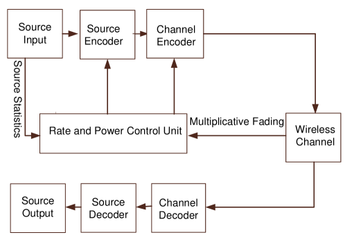
Figure 1: Block diagram of the system.

The block diagram of the system is depicted in Fig. 1. We consider $K$ source samples spanning one source block coded into a finite index by the source encoder. This index is transmitted in $N$ channel uses spanning one fading block (bandwidth expansion ratio $b=\frac{N}{K}$, here $b\in\mathbb{N}$). We assume that $K$ and $N$ are large enough such that, over a given state of source and channel, the rate distortion function of the quasi-stationary source and the instantaneous capacity of the block fading channel may be achieved. The source coding rate $R_{s}$ in bits per source sample and channel coding rate $R$ in bits per channel use are related by $R_{s}=bR$. The instantaneous capacity of the fading Gaussian channel [1] over one block (in bits per channel use) is defined as

$$C(\alpha,\gamma)=\frac{1}{2}\log_{2}(1+\alpha\gamma){.}$$ (1)

In case of a channel outage, in each state of the source and the channel $(s,\alpha)$, the instantaneous distortion is equal to the variance of the source and the decoder reconstructs the mean of the source. Whereas without channel outage, distortion is given by $\sigma^{2}_{s}2^{-2bR}$. Thus, the distortion at a given state $(s,\alpha)$ is equal to

$$D{(\sigma_{s},\alpha,\gamma)}=\begin{cases}\sigma^{2}_{s}2^{-2bR}&\text{if}\;R\leq C(\alpha,\gamma)\\ \sigma^{2}_{s}&\text{if}\;R>C(\alpha,\gamma){,}\end{cases}$$ (2)

where $C(\alpha,\gamma)$ is given in (1). Let $D_{m}$ be a nonnegative constant and represent the maximum allowable distortion. The distortion outage probability evaluated at $D_{m}$ is defined as

$$\text{P}_{\text{Dout}}=\text{Pr}(D(\sigma_{s},\alpha,\gamma)>D_{m}){,}$$ (3)

where $\gamma=\gamma(\sigma_{s},\alpha)$ is the transmission power and we have the power constraint $\text{E}[\gamma]\leq\bar{P}$.

The outage distortion exponent is defined as [14]

$$\Delta_{\textit{OD}}=\underset{\bar{P}\rightarrow\infty}{\lim}{-\frac{\ln{\text{P}_{\text{Dout}}}}{\ln{\bar{P}}}}.$$ (4)

Let $\bar{P}_{1}$ and $\bar{P}_{2}$ be the average powers transmitted to asymptotically achieve a specific distortion outage probability by two different schemes. We define the asymptotic outage distortion gain as follows

$$G\!_{O\!D}=10\log_{10}{\bar{P}_{2}}-10\log_{10}{\bar{P}_{1}}.$$ (5)

In the sequel, we also use the following mathematical definitions

$$[x]^{+}:=\operatorname{max}\{x,0\}$$ (6)

and

$$E_{1}(x):={\int^{\infty}_{x}}{\frac{e^{-\alpha}}{\alpha}\mathrm{d}\alpha},$$ (7)

as well as the following two approximations (refer to (5.1.53) in [20])

$$E_{1}(x)\cong-E_{c}-\ln(x)\quad\text{if}\;x\rightarrow 0\;,$$ (8)

where $E_{c}=0.5772156649$ is the Euler constant and

$$e^{x}\cong 1+x\quad\text{if}\;x\rightarrow 0.$$ (9)

III Channel Optimized Power Adaptation with Fixed Rate Source and Channel Coding

In this section, the aim is to find the optimized power allocation strategy and fixed rate such that the distortion outage probability for communication of a quasi-stationary source over a wireless fading channel is minimized. With a fixed rate, the encoders do not need to be rate adaptive which simplifies the design and implementation of transceivers. Noting (3) the distortion outage probability is computed as follows

$$\text{P}_{\text{Dout}}=\text{Pr}\bigl{(}R>C\left(\alpha,\gamma\right)\bigr{)}\text{Pr}\bigl{(}\sigma^{2}_{s}>D_{m}\bigr{)}+\bigl{(}1-\text{Pr}\bigl{(}R>C\left(\alpha,\gamma\right)\bigr{)}\bigr{)}\text{Pr}\bigl{(}\sigma^{2}_{s}2^{-2bR}>D_{m}\bigr{)}.$$ (10)

We have the following design problem.

Problem 1

The problem of delay-limited channel optimized power adaptation for communication of a quasi-stationary source with minimum distortion outage probability (COPA-MDO) is formulated as follows

$$\underset{\gamma,R}{\operatorname{min}}\;\text{P}_{\text{Dout}}$$

$$\text{subject to}\;\text{E}[\gamma]\leq\bar{P}{.}$$ (11)

The solution to Problem 1 is obtained in two steps. For a given fixed rate and noting $\text{Pr}\bigl{(}\sigma^{2}_{s}2^{-2bR}>D_{m}\bigr{)}\leq\text{Pr}\bigl{(}\sigma^{2}_{s}>D_{m}\bigr{)}:\forall R>0$, minimizing (10) is equivalent to minimizing $\text{Pr}\bigl{(}R>C\left(\alpha,\gamma\right)\bigr{)}$. Problem 2 below formulates this (sub)problem and provides the optimum power adaptation strategy as a function of $R$. Next, solving Problem 3, as described below, provides the optimum solution for $R$, and hence problem 1 is solved.

Problem 2

With COPA-MDO scheme and with a given fixed channel coding rate $R$, the power adaptation problem is formulated as follows

$$\begin{split}\underset{\gamma}{\operatorname{min}}\;\text{Pr}(R>C(\alpha,\gamma))\\ \text{subject to}\;\text{E}[\gamma]\leq\bar{P}{.}\end{split}$$ (12)

Proposition 1

The solution to Problem 2 for optimized power adaptation over a block fading channel is given by

$$\gamma^{*}{(\alpha,R)}=\begin{cases}\frac{2^{2R}-1}{\alpha}&\text{if}\;\;\alpha\geq\frac{2^{2R}-1}{q^{*}_{1}}\\ 0&\text{if}\;\;\alpha<\frac{2^{2R}-1}{q^{*}_{1}}{,}\end{cases}$$ (13)

in which $q^{*}_{1}$ is selected such that the power constraint is satisfied with equality, i.e.,

$$\underset{\alpha\geq\frac{2^{2R}-1}{q^{*}_{1}}}{\int}{\frac{2^{2R}-1}{\alpha}f(\alpha)\,\mathrm{d}\alpha}=\bar{P}.$$ (14)

Specifically for Rayleigh block fading channel, (14) is simplified to

$$\left(2^{2R}-1\right)E_{1}\left(\frac{2^{2R}-1}{q^{*}_{1}}\right)=\bar{P}.$$ (15)

Proof:

The proof follows that of Proposition 4 in [1]. Based on (14), for Rayleigh block fading channel $q_{1}^{*}$ is to satisfy (15). In fact $q_{1}^{*}$ sets the SNR threshold below which the channel outage occurs. ∎

Now for obtained $\gamma^{*}(\alpha,R)$, minimizing (10) is equivalent to maximizing

$$\Lambda(R)=\text{Pr}\biggl{(}R\leq C\left(\alpha,\gamma^{*}(\alpha,R)\right)\biggr{)}\biggl{(}\text{Pr}\left(\sigma^{2}_{s}>D_{m}\right)-\text{Pr}\left(\sigma^{2}_{s}2^{-2bR}>D_{m}\right)\biggr{)},$$ (16)

as formulated in Problem 3 below.

Problem 3

For COPA-MDO scheme with optimum power adaptation $\gamma^{*}(\alpha,R)$, the optimum $R$, denoted by $R^{*}$, is given by the solution to the following optimization problem

$$\begin{split}&\underset{R}{\operatorname{max}}\;\Lambda(R)\\ &\text{subject to}\;\text{E}_{\alpha}[\gamma^{*}(\alpha,R)]\leq\bar{P}.\end{split}$$ (17)

Proposition 2

Solution to Problem 3 for block fading channel is $R^{*}$, where $R^{*}$ is an element of the set $\{\frac{1}{2b}\log_{2}\frac{\sigma^{2}_{s}}{D_{m}};s\in\mathcal{S},\;\sigma^{2}_{s}\geq D_{m}\}$ that maximizes

$${\text{Pr}\left(\alpha\geq\frac{2^{2R}-1}{q^{*}_{1}}\right)\biggl{(}\text{Pr}\left(\!\sigma^{2}_{s}>D_{m}\right)-\text{Pr}\left(\sigma^{2}_{s}2^{-2bR}>D_{m}\right)\!\biggr{)}}\!$$ (18)

for $q_{1}^{*}$ satisfying (14).

Proof:

Using (1) and (13), we have

$$C(\alpha,\gamma)=\begin{cases}R&\text{if}\;\frac{2^{2R}-1}{\alpha}\leq q^{*}_{1}\\ 0&\text{if}\;\frac{2^{2R}-1}{\alpha}>q^{*}_{1}\end{cases}$$ (19)

Therefore,

$$\text{Pr}\left(R\leq C\left(\alpha,\gamma\right)\right)=\text{Pr}\left(\alpha\geq\frac{2^{2R}-1}{q^{*}_{1}}\right)$$ (20)

Thus, the maximization in Problem 3 is equivalent to

$$\underset{R}{\operatorname{max}}\;{\text{Pr}\left(\alpha\geq\frac{2^{2R}-1}{q^{*}_{1}}\right)\biggl{(}\!\text{Pr}\left(\sigma^{2}_{s}>D_{m}\right)\!-\!\text{Pr}\left(\sigma^{2}_{s}2^{-2bR}>D_{m}\right)\!\biggr{)}}\\$$ (21)

where $q_{1}^{*}$ satisfies (14).

It is clear in (21) that $\text{Pr}\left(\sigma^{2}_{s}>D_{m}\right)-\text{Pr}\left(\sigma^{2}_{s}2^{-2bR}>D_{m}\right)$ is an ascending (stair case like) function of $R$ with discontinuity at $R=\frac{1}{2b}\log_{2}\frac{\sigma^{2}_{s}}{D_{m}};\forall s\in{\mathcal{S}},\;\sigma^{2}_{s}\geq D_{m}$. On the other hand, noting (14), $\frac{\left(2^{2R}-1\right)}{q^{*}_{1}}$ increases as $R$ grows; and therefore $\text{Pr}\left(\alpha\geq\frac{2^{2R}-1}{q^{*}_{1}}\right)$ decreases as $R$ increases. Thus, the objective function in Problem 3 has discontinuities at $R=\frac{1}{2b}\log_{2}\frac{\sigma^{2}_{s}}{D_{m}};\forall s\in{\mathcal{S}},\;\sigma^{2}_{s}\geq D_{m}$ and also is a descending function of $R$ between two subsequent discontinuity points. Hence, we can conclude that the maximum of (21) occurs at one of these discontinuity points. ∎

The next two Propositions quantify the performance of the proposed COPA-MDO scheme in terms of the resulting distortion outage probability and outage distortion exponent, respectively.

Proposition 3

The distortion outage probability obtained by COPA-MDO scheme for transmission of a quasi-stationary source over a Rayleigh block fading channel is given by

$$\text{P}_{\text{Dout}}=\left(1-\exp\left(-\frac{2^{2R^{*}}-1}{q^{*}_{1}}\right)\right)\text{Pr}(\sigma^{2}_{s}>D_{m})+\exp\left(-\frac{2^{2R^{*}}-1}{q^{*}_{1}}\right)\text{Pr}(\sigma^{2}_{s}2^{-2bR^{*}}>D_{m})$$ (22)

with $q_{1}^{*}$ satisfying the following equation

$$\left(2^{2R^{*}}-1\right)E_{1}\left(\frac{2^{2R^{*}}-1}{q^{*}_{1}}\right)=\bar{P}$$ (23)

and $R^{*}$ given in Proposition 2.

Proof:

Noting (20) and with exponentially distributed channel gain, we obtain

$$\text{Pr}\left(R^{*}\leq C\left(\alpha,\gamma\right)\right)=\exp\left(-\frac{2^{2R^{*}}-1}{q^{*}_{1}}\right),$$ (24)

where $R^{*}$ is given in Proposition 2. Hence, equation (22) is derived by replacing (24) in (10). ∎

As expected, the power allocation and hence the resulting distortion outage probability are functions of the optimized fixed rate.

Proposition 4

For communication of a quasi-stationary source over a Rayleigh block fading channel, the COPA-MDO scheme achieves the outage distortion exponent $\Delta_{\textit{OD}}$ of the order $O\left(\frac{\bar{P}}{\ln{\bar{P}}}\right)$ for large average power limit $\bar{P}$.

Proof:

To compute $\Delta_{\textit{OD}}$ as defined in (4), we first note that according to (23) and Proposition 2 for large enough $\bar{P}$, we have $\frac{2^{2R^{*}}-1}{q_{1}^{*}}\rightarrow 0$. Thus, using the approximation given in (8), (23) can be rewritten as follows.

$$-\left(2^{2R^{*}}-1\right)\left(\ln\frac{2^{2R^{*}}-1}{q_{1}^{*}}+E_{c}\right)\cong\bar{P}$$ (25)

or equivalently

$$q_{1}^{*}\cong\left(2^{2R^{*}}-1\right)\exp\left(\frac{\bar{P}}{2^{2R^{*}}-1}\right).$$ (26)

Therefore, using (9) and (26) and noting $\frac{2^{2R^{*}}-1}{q_{1}^{*}}\rightarrow 0$, (22) can be rewritten as follows

$$\begin{split}\text{P}_{\text{Dout}}\cong\text{Pr}\left(\sigma^{2}_{s}>D_{m}\right)\exp\left(-\frac{\bar{P}}{2^{2R^{*}}-1}\right)+\left(1-\exp\left(-\frac{\bar{P}}{2^{2R^{*}}-1}\right)\right)\text{Pr}(\sigma^{2}_{s}2^{-2bR^{*}}>D_{m}).\end{split}$$ (27)

Noting Proposition 2 or equivalently minimizing (27) for large power constraint, it is observed that the optimum $R^{*}$ have to be set such that $\text{Pr}(\sigma^{2}_{s}2^{-2bR^{*}}>D_{m})=0$, i.e.,

$$R^{*}=\frac{1}{2b}\log_{2}\frac{\underset{s}{\operatorname{max}}\{\sigma^{2}_{s}\}}{D_{m}}$$ (28)

Thus, we have

$$\begin{split}\text{P}_{\text{Dout}}\cong\text{Pr}\left(\sigma^{2}_{s}>D_{m}\right)\exp\left(\frac{-\bar{P}}{\left(\frac{\underset{s}{\operatorname{max}}\{\sigma^{2}_{s}\}}{D_{m}}\right)^{\frac{1}{b}}-1}\right)\end{split}$$ (29)

and therefore,

$$\begin{split}\Delta_{\textit{OD}}=\underset{\bar{P}\rightarrow\infty}{\lim}{\frac{\frac{\bar{P}}{\left(\frac{\underset{s}{\operatorname{max}}\{\sigma^{2}_{s}\}}{D_{m}}\right)^{\frac{1}{b}}-1}-\ln{\text{Pr}\left(\sigma^{2}_{s}>D_{m}\right)}}{\ln{\bar{P}}}}.\end{split}$$ (30)

Hence, the proof is complete. ∎

For the optimized fixed rate $R^{*}$, the distortion outage exponent enhances when the average power limit $\bar{P}$ increases.

In the following three Corollaries, we summarize the implications of the COPA-MDO design for transmission of stationary sources over block fading channels. The stationary source is a Gaussian with zero mean and variance $\sigma^{2}\geq D_{m}$. Obviously, with $\sigma^{2}<D_{m}$, the distortion outage probability is equal to zero. The results are directly obtained from Propositions 1, 2, 3 and 4 and allows for insights into the system performance as it relates to source statistical characteristics.

Corollary 1

The optimum power adaptation and channel coding rate prescribed by COPA-MDO for transmission of a stationary source over a block fading channel are given by

$$R^{*}=\frac{1}{2b}\log_{2}{\frac{\sigma^{2}}{D_{m}}}$$ (31)

and

$$\gamma^{*}=\begin{cases}\frac{\left(\frac{\sigma^{2}}{D_{m}}\right)^{\frac{1}{b}}-1}{q^{*}_{1}}&\text{if }\alpha\geq\frac{\left(\frac{\sigma^{2}}{D_{m}}\right)^{\frac{1}{b}}-1}{q^{*}_{1}}\\ 0&\text{otherwise}\end{cases}$$ (32)

in which $q^{*}_{1}$ is selected such that the power constraint is satisfied with equality, i.e.,

$${\int_{\alpha\geq\frac{\left(\frac{\sigma^{2}}{D_{m}}\right)^{\frac{1}{b}}-1}{q^{*}_{1}}}}{\frac{\left(\frac{\sigma^{2}}{D_{m}}\right)^{\frac{1}{b}}-1}{\alpha}f(\alpha)\,\mathrm{d}\alpha}=\bar{P}.$$ (33)

Specifically for Rayleigh block fading channel, (33) is simplified to

$$\left(\left(\frac{\sigma^{2}}{D_{m}}\right)^{\frac{1}{b}}-1\right)E_{1}\left(\frac{\left(\frac{\sigma^{2}}{D_{m}}\right)^{\frac{1}{b}}-1}{q^{*}_{1}}\right)=\bar{P}.$$ (34)

Thus, for transmission of a stationary source over a block fading channel, the optimized fixed rate is simply set such that the source coding distortion is equal to its maximum $D_{m}$.

Corollary 2

The distortion outage probability obtained by COPA-MDO for transmission of a stationary source over a Rayleigh block fading channel is given by

$$\text{P}_{\text{Dout}}=1-\exp\left(-\frac{\left(\frac{\sigma^{2}}{D_{m}}\right)^{\frac{1}{b}}-1}{q^{*}}\right)$$ (35)

with $q^{*}$ satisfying the following equation

$$\left(\left(\frac{\sigma^{2}}{D_{m}}\right)^{\frac{1}{b}}-1\right)E_{1}\left(\frac{\left(\frac{\sigma^{2}}{D_{m}}\right)^{\frac{1}{b}}-1}{q^{*}}\right)=\bar{P}.$$ (36)

The results in Corollary 2 is obtained noting that $\sigma^{2}>D_{m}$ and $\text{Pr}(\sigma^{2}_{s}2^{-2bR^{*}}>D_{m})=0$ for stationary sources.

Corollary 3

For communication of a stationary source over a Rayleigh block fading channel and with large average power limit $\bar{P}$, the COPA-MDO scheme achieves the outage distortion exponent $\Delta_{\textit{OD}}=\underset{\bar{P}\rightarrow\infty}{\lim}{\frac{\bar{P}}{\ln\bar{P}\left(\left(\frac{\sigma^{2}}{D_{m}}\right)^{\frac{1}{b}}-1\right)}}$ of the order $O\left(\frac{\bar{P}}{\ln{\bar{P}}}\right)$.

This immediately follows the proof of Proposition 4 and noting that for stationary sources $R^{*}=\frac{1}{2b}\log_{2}{\frac{\sigma^{2}}{D_{m}}}$.

The performance of COPA-MDO scheme is studied and compared in Section V.

IV Source and Channel Optimized Power and Rate Adaptation

In this section, we consider power and rate adaptation with regard to source and channel states for improved performance of communications of a quasi-stationary source over a wireless block fading channel. Thus, the objective in this section is to devise power and rate adaptation strategies for each state $(s,\alpha)$ such that the distortion outage probability is minimized, when the average power is constrained to $\bar{P}$. We have the following design problem.

Problem 4

The problem of delay-limited source and channel optimized power adaptation for transmission of a quasi-stationary source with minimum distortion outage probability (SCOPA-MDO) over a block fading channel is formulated as follows

$$\begin{split}&\underset{\gamma,R}{\operatorname{min}}\;\text{P}_{\text{Dout}}=\text{Pr}\left(D(\sigma_{s},\alpha,\gamma)>D_{m}\right)\\ &\text{subject to}\;\text{E}[\gamma]<\bar{P}{,}\end{split}$$ (37)

where $D(\sigma_{s},\alpha,\gamma)$ is given in (2).

Proposition 5

The solution to Problem 4 for an arbitrary block fading channel is given by

$$\gamma^{*}{(\sigma_{s},\alpha)}=\begin{cases}\frac{1}{\alpha}\left[\left(\frac{\sigma^{2}_{s}}{D_{m}}\right)^{\frac{1}{b}}-1\right]^{+}&\text{if}\;\;\frac{1}{\alpha}\left[\left(\frac{\sigma^{2}_{s}}{D_{m}}\right)^{\frac{1}{b}}-1\right]^{+}\leq q^{*}_{2}\\ 0&\text{Otherwise}\\ \end{cases}$$ (38)

and

$$\begin{split}R=&\begin{cases}\frac{1}{2b}\log\frac{\sigma^{2}_{s}}{D_{m}}&\text{if}\;\frac{\sigma^{2}_{s}}{D_{m}}>1\;\text{and}\;\frac{1}{\alpha}\left[\left(\frac{\sigma^{2}_{s}}{D_{m}}\right)^{\frac{1}{b}}-1\right]<q^{*}_{2}\\ 0&\text{Otherwise},\end{cases}\end{split}$$ (39)

with $q^{*}_{2}$ satisfying the following equation

$$\underset{s:\sigma^{2}_{s}>D_{m}}{\sum}\underset{\alpha:\frac{1}{\alpha}\left[\left(\frac{\sigma^{2}_{s}}{D_{m}}\right)^{\frac{1}{b}}-1\right]\leq q^{*}_{2}}{\int}{\frac{\left(\frac{\sigma^{2}_{s}}{D_{m}}\right)^{\frac{1}{b}}-1}{\alpha}f(\alpha)\,P(s)\mathrm{d}\alpha}=\bar{P}.$$ (40)

Proof:

The transmission rate may be controlled with respect to the channel state. Specifically, it is logical to set the rate to its maximum as follows

$$R=C\left(\alpha,\gamma\right)=\frac{1}{2}\log(1+\alpha\gamma)$$ (41)

and therefore, we have

$$D(\sigma_{s},\alpha,\gamma)=\sigma^{2}_{s}2^{-2bR}=\frac{\sigma^{2}_{s}}{(1+\alpha\gamma)^{b}}.$$ (42)

Let $\gamma$ represent the probabilistically adapted transmission power. Obviously with distortion outage, $\gamma$ is set to zero and without distortion outage, the power is set to $\acute{\gamma}$ such that $D(\sigma_{s},\alpha,\acute{\gamma})\leq D_{m}$. We define $\omega(\sigma_{s},\alpha)$ to be the probability that (noting the channel SNR) the power is not zero in state $\sigma_{s}$ and $\alpha$. We have,

$$\gamma(\sigma_{s},\alpha)=\begin{cases}\acute{\gamma}(\sigma_{s},\alpha)&\text{with probability}\;\omega(\sigma_{s},\alpha)\\ 0&\text{with probability}\;1-\omega(\sigma_{s},\alpha).\end{cases}$$ (43)

Thus, the distortion outage probability and the average transmitted power, respectively are $1-E[\omega(\sigma_{s},\alpha)]$ and $E[\omega(\sigma_{s},\alpha)\acute{\gamma}(\sigma_{s},\alpha)]$. Hence, using a Lagrangian optimization approach, the problem may be restated as follows in which the Lagrangian variable $\lambda$ is set such that the power constraint in (37) is satisfied with equality.

$$\underset{{\omega(\sigma_{s},\alpha),\acute{\gamma}(\sigma_{s},\alpha)}}{\operatorname{max}} {E[\omega(\sigma_{s},\alpha)]-\lambda E[\omega(\sigma_{s},\alpha)\acute{\gamma}(\sigma_{s},\alpha)]}\quad\text{subject to}$$ (44)

$${C_{1}:\frac{\sigma^{2}_{s}}{(1+\alpha\acute{\gamma}(\sigma_{s},\alpha))^{b}}\leq D_{m}}$$

$${C_{2}:0<\omega(\sigma_{s},\alpha)\leq 1}.$$

Note that $\omega(\sigma_{s},\alpha)=0$ is a trivial case that is excluded in $C_{2}$ above. Due to the fact that $C_{1}$ (representing $D(\sigma_{s},\alpha,\acute{\gamma})\leq D_{m}$) and $C_{2}$ are convex, the solution to the above for $\lambda>0$ is globally optimal. To solve this problem, we first find ${\gamma}^{*}(\sigma_{s},\alpha)$ to maximize (44) for a given $\omega(\sigma_{s},\alpha)$. Then for the resulting power adaptation strategy, we obtain ${\omega}^{*}(\sigma_{s},\alpha)$ to maximize (44). Thus, ${\gamma}^{*}(\sigma_{s},\alpha)$ is the solution to

$$\begin{split}\underset{{\acute{\gamma}(\sigma_{s},\alpha)}}{\operatorname{min}}&{\lambda E[\omega(\sigma_{s},\alpha)\acute{\gamma}(\sigma_{s},\alpha)]}\quad\text{subject to}\\ &C_{1}:\frac{\sigma^{2}_{s}}{(1+\alpha\acute{\gamma}(\sigma_{s},\alpha))^{b}}\leq D_{m}.\end{split}$$ (45)

Noting $\lambda>0$ and $0<\omega(\sigma_{s},\alpha)\leq 1$, (45) is equivalent to the following

$$\begin{split}&\operatorname{min}{\acute{\gamma}(\sigma_{s},\alpha)}\\ &\text{subject to}\;\frac{\sigma^{2}_{s}}{(1+\alpha\acute{\gamma}(\sigma_{s},\alpha))^{b}}\leq D_{m}.\end{split}$$ (46)

Obviously, as ${\gamma}^{*}(\sigma_{s},\alpha)$, the solution to the problem above, is to be nonnegative, we have

$${\gamma}^{*}(\sigma_{s},\alpha)=\frac{1}{\alpha}\left[\left(\frac{\sigma^{2}_{s}}{D_{m}}\right)^{\frac{1}{b}}-1\right]^{+}.$$ (47)

Now, given the power adaptation ${\gamma}^{*}(\sigma_{s},\alpha)$, the optimization problem (44) may be rewritten as follow

$$\underset{0\leq\omega(\sigma_{s},\alpha)\leq 1}{\operatorname{max}}{\text{E}\left[\omega(\sigma_{s},\alpha)\left(1-\lambda{\gamma}^{*}(\sigma_{s},\alpha)\right)\right]}.$$ (48)

The solution to (48) is given by

$${\omega}^{*}(\sigma_{s},\alpha)=\begin{cases}1&\text{if}\;\;{\gamma}^{*}{(\sigma_{s},\alpha)}\leq\frac{1}{\lambda}\\ 0&\text{if}\;\;{\gamma}^{*}{(\sigma_{s},\alpha)}>\frac{1}{\lambda}{.}\end{cases}$$ (49)

Therefore, noting (47), (49) and (43), we obtain (38). Substituting (38) in (41), achieving (39) is straightforward.

The Lagrangian variable $\lambda$ is set such that the power constraint $\text{E}[{\omega}^{*}(\sigma_{s},\alpha){\gamma}^{*}(\sigma_{s},\alpha)]=\bar{P}$ is satisfied. We have

$$\underset{s\in{\mathcal{S}}}{\sum}\underset{\alpha:{\gamma}^{*}(\sigma_{s},\alpha)\leq\frac{1}{\lambda}}{\int}{{\gamma}^{*}(\sigma_{s},\alpha)f(\alpha)\,P(s)\mathrm{d}\alpha}=\bar{P},$$ (50)

where replacing $\frac{1}{\lambda}$ with $q^{*}_{2}$ completes the proof. ∎

The next two Propositions quantify the performance of the proposed SCOPA-MDO scheme in terms of the resulting distortion outage probability and outage distortion exponent, respectively.

Proposition 6

The distortion outage probability for transmission of a quasi-stationary source using the SCOPA-MDO scheme over a Rayleigh block fading channel is given by

$$\text{P}_{\text{Dout}}=\text{Pr}(\sigma^{2}_{s}>D_{m})\!-\!\underset{s:\sigma^{2}_{s}>D_{m}}{\sum}\!\exp{\left(-\frac{\left(\frac{\sigma^{2}_{s}}{D_{m}}\right)^{\frac{1}{b}}\!-\!1}{q^{*}_{2}}\right)}P(s)$$ (51)

with $q^{*}_{2}$ satisfying the following equation

$$\begin{split}\underset{s:\sigma^{2}_{s}>D_{m}}{\sum}{\left(\left(\frac{\sigma^{2}_{s}}{D_{m}}\right)^{\frac{1}{b}}-1\right)E_{1}\left(\frac{\left(\frac{\sigma^{2}_{s}}{D_{m}}\right)^{\frac{1}{b}}-1}{q^{*}_{2}}\right)P(s)}=\bar{P}.\end{split}$$ (52)

Proof:

The proof is provided in Appendix A. ∎

Proposition 7

For communication of a quasi-stationary source over a Rayleigh block fading channel, the SCOPA-MDO scheme achieves an outage distortion exponent $\Delta_{\textit{OD}}$ of the order $O\left({\frac{\bar{P}}{\ln{\bar{P}}}}\right)$ for large average power limit $\bar{P}$.

Proof:

Noting (52), $\bar{P}\rightarrow\infty$ requires that $q^{*}_{2}\rightarrow\infty$. In this case, using (8), we can rewrite (52) as follows.

$$\begin{split}\underset{s:\sigma^{2}_{s}>D_{m}}{\sum\!}{\!-\left(\left(\frac{\sigma^{2}_{s}}{D_{m}}\right)^{\frac{1}{b}}-1\right)\ln\frac{\left(\frac{\sigma^{2}_{s}}{D_{m}}\right)^{\frac{1}{b}}-1}{q^{*}_{2}}P(s)}\cong\bar{P}\end{split}$$ (53)

and after some manipulations, we obtain

$$\begin{split}q^{*}_{2}\cong\exp\left(\frac{\bar{P}}{\underset{s:\sigma^{2}_{s}>D_{m}}{\sum}{\left(\left(\frac{\sigma^{2}_{s}}{D_{m}}\right)^{\frac{1}{b}}-1\right)P(s)}}\right).\exp\!\left(\!\frac{\!\underset{s:\sigma^{2}_{s}>D_{m}}{\sum}{\!\left(\left(\frac{\sigma^{2}_{s}}{D_{m}}\right)^{\frac{1}{b}}-1\right)\ln\left(\!\left(\frac{\sigma^{2}_{s}}{D_{m}}\!\right)^{\frac{1}{b}}-1\right)\!P(s)}\!}{\underset{s:\sigma^{2}_{s}>D_{m}}{\sum}{\!\left(\left(\frac{\sigma^{2}_{s}}{D_{m}}\right)^{\frac{1}{b}}-1\right)\!P(s)}}\!\right).\end{split}$$ (54)

Considering (51) and (9) for $q^{*}_{2}\rightarrow\infty$, we have

$$\text{P}_{\text{Dout}}\cong\frac{1}{q^{*}_{2}}\underset{s:\sigma^{2}_{s}>D_{m}}{\sum}{\left(\left(\frac{\sigma^{2}_{s}}{D_{m}}\right)^{\frac{1}{b}}-1\right)P(s)}.$$ (55)

Hence, noting (54) for $q^{*}_{2}\rightarrow\infty$ we obtain

$$\begin{split}\Delta_{\textit{OD}}=\underset{\bar{P}\rightarrow\infty}{\lim}{\frac{\bar{P}}{\ln{\bar{P}}\underset{s:\sigma^{2}_{s}>D_{m}}{\sum}{\left(\left(\frac{\sigma^{2}_{s}}{D_{m}}\right)^{\frac{1}{b}}-1\right)P(s)}}}.\end{split}$$ (56)

Thus, the proof is completed. ∎

The following Corollary expresses the implication of the SCOPA-MDO design for transmission of a stationary source over block fading channels. This is directly obtained from Proposition 5 when a stationary source is assumed.

Corollary 4

The optimum channel coding rate and power adaptation prescribed by SCOPA-MDO for transmission of a stationary source over a block fading channel are given by

$$R^{*}=\begin{cases}\frac{1}{2b}\log_{2}{\frac{\sigma^{2}}{D_{m}}}&\text{if }\alpha\geq\frac{\left(\frac{\sigma^{2}}{D_{m}}\right)^{\frac{1}{b}}-1}{q^{*}_{2}}\\ 0&\text{otherwise}\end{cases}$$ (57)

$$\gamma^{*}=\begin{cases}\frac{\left(\frac{\sigma^{2}}{D_{m}}\right)^{\frac{1}{b}}-1}{q^{*}_{2}}&\text{if }\alpha\geq\frac{\left(\frac{\sigma^{2}}{D_{m}}\right)^{\frac{1}{b}}-1}{q^{*}_{2}},\\ 0&\text{otherwise}\end{cases}$$ (58)

in which $q^{*}_{2}$ is selected such that the power constraint is satisfied with equality, i.e.,

$$\underset{\alpha\geq\frac{\left(\frac{\sigma^{2}}{D_{m}}\right)^{\frac{1}{b}}-1}{q^{*}_{2}}}{\int}{\frac{\left(\frac{\sigma^{2}}{D_{m}}\right)^{\frac{1}{b}}-1}{\alpha}f(\alpha)\,\mathrm{d}\alpha}=\bar{P}.$$ (59)

Specifically for Rayleigh block fading channel, (59) is simplified to

$$\left(\left(\frac{\sigma^{2}}{D_{m}}\right)^{\frac{1}{b}}-1\right)E_{1}\left(\frac{\left(\frac{\sigma^{2}}{D_{m}}\right)^{\frac{1}{b}}-1}{q^{*}_{2}}\right)=\bar{P}.$$ (60)

Remark 1

Examining Corollaries 1 and 4 for transmission of a stationary source over a block fading channel, one sees that the SCOPA-MDO and COPA-MDO schemes provide the same distortion outage probability and outage distortion exponent. This implies that in this setting with power adaptation an optimized fixed rate provides all the gain that may be obtained by rate adaptation.

The performance of SCOPA-MDO scheme is studied in Section V.

V Performance Evaluation

In this section, we first present two constant power transmission schemes as benchmarks for comparisons. Next, we consider analytical performance comparison of different schemes followed by numerical results. To this end, we consider four quasi-stationary sources, with $N_{s}=25$ where the variance of the source in the state $s$ is given by $\sigma^{2}_{s}(s)=(1+\frac{1}{6}s)^{2}:\forall{s}\in\{0,1,...,N_{S}-1\}$. For three of the sources, labeled as G1, G2 and G3, the probability of being in different states follows a discrete Gaussian distribution with mean 3 and variances 0.05, 0.48, 1.07, respectively. For the fourth source, U, the said distribution is considered uniform with the same mean and a variance of 1.44. We also consider an stationary source S with $\sigma_{s}=3$ for a meaningful comparison. Unless otherwise mentioned, we consider the source G2 for the following results and simulations.

V-A Benchmark

Two constant power schemes for transmission of a quasi-stationary source over a block fading channel are considered as benchmarks for comparisons. In the first scheme, the channel coding rate is adjusted based on the channel state to minimize the distortion outage probability; hence the scheme is labeled as Channel Optimized Rate Adaptation with Constant Power (CORACP). In the second scheme with Constant Rate and Constant Power (CRCP), the aim is to find the optimized fixed rate such that the distortion outage probability is minimized.

V-A1 Channel Optimized Rate Adaptation with Constant Power

With CORACP and constant transmission power $\bar{P}$, the instantaneous capacity is given by $C=\frac{1}{2}\log_{2}{\left(1+\alpha\bar{P}\right)}$; and hence to minimize $\text{P}_{\text{Dout}}$ it is logical to consider the rate adaptation strategy of $R=C$. The source coding rate is then set as $R_{s}=bR$. The next two Propositions quantify the distortion outage performance of CORACP.

Proposition 8

The distortion outage probability for transmission of a quasi-stationary source over a Rayleigh block fading channel using CORACP is given by

$$\begin{split}\text{P}_{\text{Dout}}=\text{Pr}(\sigma^{2}_{s}>D_{m})-\underset{s:\sigma^{2}_{s}>D_{m}}{\sum}\exp\left(-\frac{1}{\bar{P}}\left[\left(\frac{\sigma^{2}_{s}}{D_{m}}\right)^{\frac{1}{b}}-1\right]\right)P(s){.}\end{split}$$ (61)

Proof:

The proof is provided in Appendix B. ∎

Proposition 9

For communication of a quasi-stationary source over a Rayleigh block fading channel, the CORACP scheme achieves the outage distortion exponent $\Delta_{\textit{OD}}$ of the order $O\left(1\right)$.

Proof:

Using (9) and considering large enough $\bar{P}$, (61) can be rewritten as

$$\text{P}_{\text{Dout}}\cong\frac{1}{\bar{P}}\underset{s:\sigma^{2}_{s}>D_{m}}{\sum}\left(\left(\frac{\sigma^{2}_{s}}{D_{m}}\right)^{\frac{1}{b}}-1\right)P(s).$$ (62)

Thus,

$$\begin{split}\Delta_{\textit{OD}}=\underset{\bar{P}\rightarrow\infty}{\lim}{-\frac{-\ln{\bar{P}}+\ln{\underset{s:\sigma^{2}_{s}>D_{m}}{\sum}\left(\left(\frac{\sigma^{2}_{s}}{D_{m}}\right)^{\frac{1}{b}}-1\right)P(s)}}{\ln{\bar{P}}}}=1\end{split}$$ (63)

and the proof is complete. ∎

Based on Propositions 8 and 9, the following Corollary presents the performance of CORACP with stationary sources.

Corollary 5

For communication of a stationary source over a Rayleigh block fading channel, the CORACP scheme achieves a distortion outage probability of

$$\text{P}_{\text{Dout}}=1-\exp\left(-\frac{\left(\frac{\sigma^{2}}{D_{m}}\right)^{\frac{1}{b}}-1}{\bar{P}}\right)$$ (64)

and an outage distortion exponent of $\Delta_{\textit{OD}}$ of the order $O\left(1\right)$.

V-A2 Constant Rate Constant Power

With CRCP, the fixed rate is optimized to minimize the distortion outage probability when the power is constant. The following three Propositions express the optimized fixed rate, distortion outage probability and distortion outage exponent obtained by CRCP.

Proposition 10

For transmission of a quasi-stationary source over a block fading channel using the CRCP scheme, the optimum rate, $R^{*}$, is an element of the set $\{\frac{1}{2b}\log_{2}\frac{\sigma^{2}_{s}}{D_{m}};s\in\mathcal{S},\;\sigma^{2}_{s}\geq D_{m}\}$ that maximizes

$${\text{Pr}\left(\alpha\geq\frac{2^{2R}-1}{\bar{P}}\right)\biggl{(}\text{Pr}\left(\!\sigma^{2}_{s}>D_{m}\right)-\text{Pr}\left(\sigma^{2}_{s}2^{-2bR}>D_{m}\right)\!\biggr{)}}\!$$ (65)

Proof:

The proof is similar to the proof of Proposition 3. ∎

Proposition 11

For transmission of a quasi-stationary source over a Rayleigh block fading channel, the CRCP scheme achieves the distortion outage probability of

$$\text{P}_{\text{Dout}}=\left(1-\exp\left(-\frac{2^{2R^{*}}-1}{\bar{P}}\right)\right)\text{Pr}(\sigma^{2}_{s}>D_{m})+\exp\left(-\frac{2^{2R^{*}}-1}{\bar{P}}\right)\text{Pr}(\sigma^{2}_{s}2^{-2bR^{*}}>D_{m}),$$ (66)

with $R^{*}$ in Proposition 10, and the outage distortion exponent $\Delta_{\textit{OD}}$ of the order $O\left(1\right)$.

Proof:

Noting (10) and constant power $\bar{P}$ with exponentially distributed channel gain, obtaining $\text{P}_{\text{Dout}}$ is straightforward. For a large power constraint, one can verify that $R^{*}$ is simplified to

$$R^{*}=\frac{1}{2b}\log_{2}\frac{\underset{s}{\operatorname{max}}\{\sigma^{2}_{s}\}}{D_{m}}.$$ (67)

Thus, from Proposition 11 and noting (9) and (67), we obtain

$$\begin{split}\text{P}_{\text{Dout}}\cong\frac{\left(\frac{\underset{s}{\operatorname{max}}\{\sigma^{2}_{s}\}}{D_{m}}\right)^{\frac{1}{b}}-1}{\bar{P}}\text{Pr}\left(\sigma^{2}_{s}>D_{m}\right)\end{split}$$ (68)

and therefore,

$$\begin{split}\Delta_{\textit{OD}}=\underset{\bar{P}\rightarrow\infty}{\lim}{-\frac{-\ln(\bar{P})+\ln\left(\left({\left(\frac{\underset{s}{\operatorname{max}}\{\sigma^{2}_{s}\}}{D_{m}}\right)^{\frac{1}{b}}-1}\right)\text{Pr}\left(\sigma^{2}_{s}>D_{m}\right)\right)}{\ln{\bar{P}}}}=1.\end{split}$$ (69)

∎

Based on the above two Propositions, the following two Corollaries present the optimum rate and the performance of CRCP with stationary sources.

Corollary 6

The optimum channel coding rate prescribed by CRCP for transmission of a stationary source over a block fading channel is given by

$$R^{*}=\frac{1}{2b}\log_{2}{\frac{\sigma^{2}}{D_{m}}}$$ (70)

Corollary 7

For communication of a stationary source over a Rayleigh block fading channel, the CRCP scheme achieves a distortion outage probability of

$$\text{P}_{\text{Dout}}=1-\exp\left(-\frac{\left(\frac{\sigma^{2}}{D_{m}}\right)^{\frac{1}{b}}-1}{\bar{P}}\right)$$ (71)

and an outage distortion exponent of $\Delta_{\textit{OD}}$ of the order $O\left(1\right)$.

Remark 2

Noting Corollaries 5 and 7 for transmission of a stationary source over a block fading channel, one sees that the CORACP and CRCP schemes provide the same distortion outage probability and outage distortion exponent. This implies that in this setting with constant power, an optimized fixed rate provides all the gain that may be obtained by rate adaptation.

V-B Analytical Performance Comparison

In the sequel, we quantify the respective asymptotic outage distortion gain $G_{\textit{OD}}$ of SCOPA-MDO, COPA-MDO, CORACP and CRCP for transmission of a quasi-stationary source over a block fading channel.

Proposition 12

In transmission of a quasi-stationary source over a Rayleigh block fading channel, the asymptotic outage distortion gain obtained by SCOPA-MDO with respect to COPA-MDO is given by

$$G\!_{O\!D}=10\log_{10}\left(\left(\frac{\underset{s}{\operatorname{max}}\{\sigma^{2}_{s}\}}{D_{m}}\right)^{\frac{1}{b}}-1\right)-10\log_{10}{\underset{s:\sigma^{2}_{s}>D_{m}}{\sum}{\left(\left(\frac{\sigma^{2}_{s}}{D_{m}}\right)^{\frac{1}{b}}-1\right)P(s)}}.$$ (72)

Proof:

The proof is provided in Appendix C. ∎

Proposition 13

In transmission of a quasi-stationary source over a Rayleigh block fading channel, the asymptotic outage distortion gain obtained by COPA-MDO with respect to CORACP is given by

$$G\!_{O\!D}=10\log_{10}{\frac{\bar{P}_{2}}{\left(\frac{\underset{s}{\operatorname{max}}\{\sigma^{2}_{s}\}}{D_{m}}\right)^{\frac{1}{b}}-1}}-10\log_{10}{\ln{\frac{\bar{P}_{2}}{\underset{s:\sigma^{2}_{s}>D_{m}}{\sum}{\left(\left(\frac{\sigma^{2}_{s}}{D_{m}}\right)^{\frac{1}{b}}-1\right)P(s)}}}},$$ (73)

where $\bar{P}_{1}$ and $\bar{P}_{2}$ are power limits in COPA-MDO and CORACP; $\bar{P}_{1}(\rm{dB})=$$\bar{P}_{2}(\rm{dB})$-$G\!_{O\!D}$.

Proof:

The proof is provided in Appendix C. ∎

Proposition 14

In transmission of a quasi-stationary source over a Rayleigh block fading channel, the asymptotic outage distortion gain obtained by CORACP with respect to CRCP is given by

$$G\!_{O\!D}=10\log_{10}\left(\left(\left(\frac{\underset{s}{\operatorname{max}}\{\sigma^{2}_{s}\}}{D_{m}}\right)^{\frac{1}{b}}-1\right)\text{Pr}\left(\sigma^{2}_{s}>D_{m}\right)\right)-10\log_{10}{\underset{s:\sigma^{2}_{s}>D_{m}}{\sum}{\left(\left(\frac{\sigma^{2}_{s}}{D_{m}}\right)^{\frac{1}{b}}-1\right)P(s)}}.$$ (74)

Proof:

The proof is provided in Appendix C. ∎

As evident, $G_{\textit{OD}}$ of SCOPA-MDO with respect to COPA-MDO and CORACP with respect to CRCP are independent of the power. This is while the gain of COPA-MDO with respect to CORACP depends nonlinearly on the average transmission power limit and it improves when the power limit increases. The dependency of $G_{\textit{OD}}$ on the variance of the source in different states and the maximum allowable distortion is also seen in (72) to (74). Table I presents the value of $G\!_{O\!D}$ at $D_{m}=8\rm dB$.

The distortion outage exponent $\Delta_{\textit{OD}}$ of the COPA-MDO and SCOPA-MDO schemes which are derived in line with the proofs of the Propositions 4 and 7, are quantified in Table II. As denoted in Propositions 9 and 11, CORACP and CRCP schemes give $\Delta_{\textit{OD}}=1$. The distortion outage exponent indicates the speed at which the distortion outage ($\rm dB$) reduces as the average power (limit) ($\rm dB$) increases. Therefore, as evident, this speed is noticeably high with SCOPA-MDO and very low with CORACP and CRCP. Furthermore, the $\Delta_{\textit{OD}}$ obtained by SCOPA-MDO and COPA-MDO depends on the average power limit $\bar{P}$, maximum allowable distortion $D_{m}$ and bandwidth expansion ratio $b$. It is observed that with SCOPA-MDO and COPA-MDO, $\Delta_{\textit{OD}}$ improves as $b$, $\bar{P}$ or $D_{m}$ increase. In fact, for a given value of $N$, a larger $b$ implies a more finely encoded source that is more sensitive to channel errors and hence can more greatly benefit from increased power. The results in Tables I and II indicate that from the perspective of probability of distortion outage, for delay-limited communication of quasi-stationary sources, CORACP and CRCP schemes may not be appropriate designs.

TABLE I: Asymptotic outage distortion gain $G\!_{O\!D}$ of scheme 1 with respect to scheme 2 for source G2 evaluated at $b=1$ and $D_{m}=8\rm dB$.

Scheme 1	Scheme 2	$G\!_{O\!D}$ at $\bar{P}_{2}=25\rm dB$	$G\!_{O\!D}$ at $\bar{P}_{2}=20\rm dB$
SCOPA-MDO	COPA-MDO	7.14	7.14
COPA-MDO	CORACP	12.28	8.16
CORACP	CRCP	5.74	5.74

TABLE II: Distortion outage exponent $\Delta_{\textit{OD}}$ of the proposed schemes for source G2

Bandwidth Expansion Ratio	$b$=1		$b$=5
Schemes and Settings	SCOPA-MDO	COPA-MDO	SCOPA-MDO	COPA-MDO
$\tiny{D_{m}}=8\rm dB$, $\tiny{\bar{P}=16\rm dB}$	18.90	3.89	129.08	34.33
$\tiny{D_{m}=8\rm dB}$, $\tiny{\bar{P}=20\rm dB}$	37.97	7.53	259.39	68.69
$\tiny{D_{m}=5\rm dB}$, $\tiny{\bar{P}=20\rm dB}$	10.80	3.27	95.75	42.53

The following three Corollaries quantify the asymptotic outage distortion gain in transmission of a stationary source over block fading channels. These are directly obtained from Propositions 12 and 14 when a stationary source is considered.

Corollary 8

In transmission of a stationary source over a Rayleigh block fading channel, the asymptotic outage distortion gain obtained by SCOPA-MDO with respect to COPA-MDO is equal to zero.

Corollary 9

In transmission of a stationary source over a Rayleigh block fading channel, the asymptotic outage distortion gain of COPA-MDO with respect to CORACP is equal to

$$G\!_{O\!D}=10\log_{10}{\frac{X}{\ln{X}}},$$ (75)

where $X:=\frac{\bar{P}_{2}}{\left(\frac{\sigma^{2}}{D_{m}}\right)^{\frac{1}{b}}-1}$ and $\bar{P}_{2}$ is the power limit of CORACP.

Corollary 10

In transmission of a stationary source over a Rayleigh block fading channel, the asymptotic outage distortion gain of CORACP with respect to CRCP is equal to zero.

The values of $G\!_{O\!D}$ in (75) and $\Delta_{\textit{OD}}$ in Corollary 3 for the stationary source S, $\bar{P}_{2}=20\rm dB$ and $D_{m}=8\rm dB$ respectively amount to $16.33\rm dB$ and $51$. Noting Remarks 1 and 2, it is observed that with stationary sources and common settings, an optimized fixed rate scheme and an adaptive rate scheme provide the same distortion outage probability. Therefore, in this setting, with optimum power adaptation, COPA-MDO and SCOPA-MDO schemes; and with constant power, CORACP and CRCP schemes provide the same distortion outage probability.

V-C Numerical Results

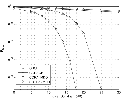
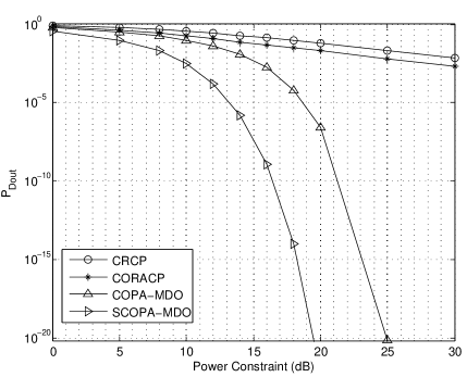
(a)	(b)

Figure 2: Distortion outage probability versus $\bar{P}$; $b=1$ and (a) $D_{m}=\rm 8\,dB$ (b)$D_{m}=\rm 5\,dB$.

Figs. 2a and 2b depict the distortion outage probability performance of the presented schemes as a function of the power constraint $\bar{P}$ for $D_{m}=\rm 8\,dB$ and $D_{m}=\rm 5\,dB$, respectively. As expected, for a given $\bar{P}$, $\text{P}_{\text{Dout}}$ decreases as $D_{m}$ increases. It is evident that the proposed SCOPA-MDO scheme achieves an asymptotic outage distortion gain of about $\rm 7.1\,dB$ and $\rm 5.6\,dB$ with respect to COPA-MDO, for $\bar{P}=\rm 20\,dB$ and $D_{m}=\rm 8\,dB$ and $D_{m}=\rm 5\,dB$, respectively. In the same settings, the COPA-MDO scheme achieves asymptotic outage distortion gains of about $\rm 9.1\,dB$ and $\rm 6.3\,dB$ with respect to CORACP; and CORACP achieves gains of $\rm 6\,dB$ and $\rm 4.9\,dB$ with respect to CRCP. The results obtained from simulations and what is reported in Table I from analyses match reasonably well given the assumption of very high average SNR considered in the analytical performance evaluations.

The analytical results in Table II for $\Delta_{\textit{OD}}$ performance, may also be observed in numerical results of Figs. 2a and 2b. Specifically, at each point on the curves, the corresponding value in the vertical coordinate in $\rm dB$, i.e., $10\log_{10}{\text{P}_{\text{Dout}}}$ divided by the value in the horizontal coordinate, i.e., $\bar{P}(\rm dB)$, indicates $-\Delta_{\textit{OD}}$. For example, as seen in Fig. 2b, $\Delta_{\textit{OD}}$ for SCOPA-MDO is almost equal to $38$ at $\bar{P}=20\rm\,dB$ with $D_{m}=8\rm\,dB$.

Figs. 3a and 3b depict the $\text{P}_{\text{Dout}}$ performance of the presented schemes for different sources. As observed, as the non-stationary characteristics of the source intensifies (from source S to U), the distortion outage probability increases in general. However, the sensitivity of the performance of different schemes to the level of non-stationarity varies. Once again, the advantage of power adaptation is clear. For the stationary source S, as noted in Remarks 1 and 2 and also seen in these Figures, SCOPA-MDO and COPA-MDO schemes provide the same distortion outage probability in this setting. This also holds true for CORACP and CRCP. It is observed that SCOPA-MDO (or equivalently COPA-MDO) scheme achieves an asymptotic outage distortion gain of about $\rm 16.8\,dB$ with respect to CORACP (or equivalently CRCP) for $\bar{P}=\rm 20\,dB$ and $D_{m}=\rm 8\,dB$.

It is noteworthy that the four methods discussed, rely on different levels of source and channel state information (SSI and CSI). Specifically, it can be verified that three schemes of SCOPA-MDO, COPA-MDO and CORACP require instantaneous CSI for rate and/or power adaptation, while CRCP needs CSI statistics. The SCOPA-MDO scheme also needs instantaneous SSI, while COPA-MDO and CRCP simply need SSI statistics.

VI Conclusions

In this paper, delay-limited transmission of a quasi-stationary source over a block fading channel was considered. Aiming at minimizing the distortion outage probability, two transmission strategies namely channel-optimized power adaptation with fixed rate (COPA-MDO) and source and channel optimized power (and rate) adaptation (SCOPA-MDO) were introduced. The SCOPA-MDO scheme provides a superior performance, while the COPA-MDO scheme enjoys the simplicity of single rate transmission. In high SNR regime, different scaling laws involving outage distortion exponent and asymptotic outage distortion were derived. Our studies confirm the benefit of power adaption from a distortion outage perspective and for delay-limited transmission of quasi-stationary sources over wireless block fading channels. The analyses of the presented schemes in the case of stationary sources indicate the same outage distortion performance with or without rate adaptation.

Appendix A Proof of Proposition 6

Noting (40) and (7) for exponentially distributed channel gain, we can obtain (52) and subsequently $q^{*}_{2}$ by numerical methods. Using (38) and (42), the distortion for each state of the source and the channel is given by

$$D(\sigma_{s},\alpha,\gamma)=\begin{cases}D_{m}&\text{if}\;\frac{\sigma^{2}_{s}}{D_{m}}>1\;\text{and}\;\frac{\left[\left(\frac{\sigma^{2}_{s}}{D_{m}}\right)^{\frac{1}{b}}-1\right]}{\alpha}<q^{*}_{2}\\ \sigma^{2}_{s}&\text{otherwise}{.}\end{cases}$$ (76)

Therefore, we have

$$\text{P}_{\text{Dout}}=\text{Pr}\left(\frac{1}{\alpha}\left[\left(\frac{\sigma^{2}_{s}}{D_{m}}\right)^{\frac{1}{b}}-1\right]\geq q^{*}_{2},\,\sigma^{2}_{s}>D_{m}\right).$$ (77)

Considering exponentially distributed channel gain $\alpha$, deriving (51) is straightforward.

Appendix B Proof of Proposition 8

Noting (42) for $\gamma=\bar{P}$, distortion can be written as follows

$$D(\sigma_{s},\alpha,\gamma=\bar{P})=\sigma^{2}_{s}2^{-2bR}=\frac{\sigma^{2}_{s}}{\left(1+\alpha\bar{P}\right)^{b}}$$ (78)

and then we can derive

$$\begin{split}\text{P}_{\text{Dout}}&=\text{Pr}\left(\frac{\sigma^{2}_{s}}{\left(1+\alpha\bar{P}\right)^{b}}>D_{m},\sigma^{2}_{s}>D_{m}\right)=\text{Pr}\left(\alpha<\frac{1}{\bar{P}}\left(\left(\frac{\sigma^{2}_{s}}{D_{m}}\right)^{\frac{1}{b}}-1\right),\sigma^{2}_{s}>D_{m}\right).\end{split}$$ (79)

Considering exponentially distributed channel gain $\alpha$, obtaining (61) is straightforward.

Appendix C Proof of Propositions 12 and 13

The average power to asymptotically achieve a certain distortion outage probability using SCOPA-MDO and COPA-MDO schemes are denoted by $\bar{P}_{1}$ and $\bar{P}_{2}$, respectively. Thus, we can use (5) to derive $G\!_{O\!D}$. Noting (54), (55) and (29) we set

$$\begin{split}\underset{\bar{P_{1}}\rightarrow\infty}{\lim}\frac{\bar{P}_{1}}{\underset{s:\sigma^{2}_{s}>D_{m}}{\sum}{\left(\left(\frac{\sigma^{2}_{s}}{D_{m}}\right)^{\frac{1}{b}}-1\right)P(s)}}=\underset{\bar{P_{2}}\rightarrow\infty}{\lim}\frac{\bar{P}_{2}}{\left(\frac{\underset{s}{\operatorname{max}}\{\sigma^{2}_{s}\}}{D_{m}}\right)^{\frac{1}{b}}-1}.\end{split}$$ (80)

Therefore, we can derive (72) and complete the proof of Proposition 12.

The proof of Propositions 13 or 14 is straightforward, when we use (29) and (62) or (62) and (68); and obtain the following

$$\begin{split}\underset{\bar{P_{2}}\rightarrow\infty}{\lim}\frac{\bar{P}_{1}}{\left(\frac{\underset{s}{\operatorname{max}}\{\sigma^{2}_{s}\}}{D_{m}}\right)^{\frac{1}{b}}-1}=\underset{\bar{P}_{2}\rightarrow\infty}{\lim}\ln{\frac{\bar{P}_{2}}{\underset{s:\sigma^{2}_{s}>D_{m}}{\sum}{\left(\left(\frac{\sigma^{2}_{s}}{D_{m}}\right)^{\frac{1}{b}}-1\right)P(s)}}}\end{split}$$ (81)

$$\underset{\bar{P}_{2}\rightarrow\infty}{\lim}{\frac{\bar{P}_{1}}{\underset{s:\sigma^{2}_{s}>D_{m}}{\sum}{\left(\left(\frac{\sigma^{2}_{s}}{D_{m}}\right)^{\frac{1}{b}}-1\right)P(s)}}}=\underset{\bar{P_{2}}\rightarrow\infty}{\lim}{\frac{\bar{P}_{2}}{\left(\left(\frac{\underset{s}{\operatorname{max}}\{\sigma^{2}_{s}\}}{D_{m}}\right)^{\frac{1}{b}}-1\right)\text{Pr}\left(\sigma^{2}_{s}>D_{m}\right)}}.$$ (82)

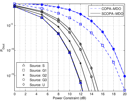
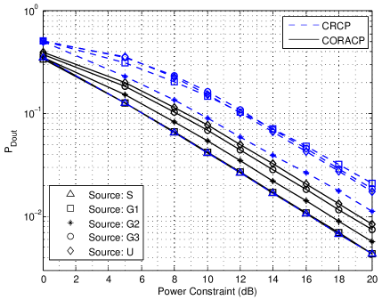
(a)	(b)

Figure 3: Distortion outage probability versus $\bar{P}$ for five different sources; $b=1$ and $D_{m}=\rm 8\,dB$.

​

References

- [1] G. Caire, G. Taricco, and E. Biglieri, “Optimum power control over fading channels,” IEEE Trans. Inform. Theory, vol. 45, pp. 1468–1489, July 1999.
- [2] V. Hanly and D. Tse, “Multiaccess fading channels. Part II: Delay-limited capacities,” IEEE Trans. Inform. Theory, vol. 44, pp. 2816–2831, Nov. 1998.
- [3] L. Li and A. J. Goldsmith, “Capacity and optimal resource allocation for fading broadcast channels. Part II: Outage capacity,” IEEE Trans. Inform. Theory, vol. 47, pp. 1103–1127, Mar. 2001.
- [4] L. Li, N. Jindal, and A. Goldsmith, “Outage capacities and optimal power allocation for fading multiple-access channels,” IEEE Trans. Inform. Theory, vol. 51, pp. 1326–1347, Nov. 2005.
- [5] J. N. Laneman, D. N. C. Tse, and G. W. Wornell, “Cooperative diversity in wireless networks: Efficient protocols and outage behavior,” IEEE Trans. Inform. Theory, vol. 50, pp. 3062–3080, Nov. 2004.
- [6] Y. Liang, V. V. Veeravalli, and H. V. Poor, “Resource allocation for wireless fading relay channels: Max-Min solution,” IEEE Trans. Inform. Theory, vol. 53, pp. 3432–3453, Oct. 2007.
- [7] D. Gunduz and E. Erkip, “Opportunistic cooperation by dynamic resource allocation,” IEEE Trans. Wireless Commun., vol. 6, pp. 1446–1454, Oct. 2007.
- [8] J. N. Laneman, G. W. Wornell, and J. G. Apostolopoulos, “Source-channel diversity for parallel channels,” IEEE Trans. Inform. Theory, vol. 51, pp. 3518–3539, Oct. 2005.
- [9] B. Dunn and J. N. Laneman, “Characterizing source-channel diversity approaches beyond the distortion exponent,” in 43rd Annu. Allerton Conf. Communications, Control and Computing, (Monticello, IL), Oct. 2005.
- [10] D. Gunduz and E. Erkip, “Joint source-channel codes for MIMO block-fading channels,” IEEE Trans. Inform. Theory, vol. 54, pp. 116–134, Jan. 2008.
- [11] D. Gunduz and E. Erkip, “Source and channel coding for cooperative relaying,” IEEE Trans. Inform. Theory, vol. 53, pp. 3454–3475, Oct. 2007.
- [12] T. Holliday, A. J. Goldsmith, and H. V. Poor, “Joint source and channel coding for MIMO systems: Is it better to be robust or quick?,” IEEE Trans. Inform. Theory, vol. 54, pp. 1393–1405, Apr. 2008.
- [13] K. Bhattad, K. R. Narayanan, and G. Caire, “On the distortion SNR exponent of some layered transmission schemes,” IEEE Trans. Inform. Theory, vol. 54, pp. 2943–2958, July 2008.
- [14] L. Peng and A. Guillen i Fabregas, “Distortion outage probability in MIMO block-fading channels,” in IEEE Int. Symp. Inform. Theory, (Austin, Texas, U.S.A), pp. 2223–2227, June 2010.
- [15] D. Gunduz, E. Erkip, A. Goldsmith, and H. V. Poor, “Source and channel coding for correlated sources over multiuser channels,” IEEE Trans. Inform. Theory, vol. 55, pp. 3927–3944, Sept. 2009.
- [16] S. Vembu, S. Verdu, and Y. Steinberg, “The source-channel separation theorem revisited,” IEEE Trans. Inform. Theory, vol. 41, pp. 44–54, Jan. 1995.
- [17] M. Alouini and A. Goldsmith, “Capacity of Rayleigh fading channels under different adaptive transmission and diversity-combining techniques,” IEEE Trans. Veh. Technol., vol. 48, pp. 1165–1181, July 1996.
- [18] Z. He, Y. Liang, L. Chen, I. Ahmad, and D. Wu, “Power-rate-distortion analysis for wireless video communication under energy constraints,” IEEE Trans. Circuits Syst. Video Technol., vol. 15, pp. 1468–1489, May 2005.
- [19] T. M. Cover and J. A. Thomas, Elements of Information Theory. New York: Wiley, 1991.
- [20] M. Abramowitz and I. A. Stegun, Handbook of Mathematical Functions. June 1974.