A class of covariate-dependent spatiotemporal covariance functions for the analysis of daily ozone concentration

Abstract

In geostatistics, it is common to model spatially distributed phenomena through an underlying stationary and isotropic spatial process. However, these assumptions are often untenable in practice because of the influence of local effects in the correlation structure. Therefore, it has been of prolonged interest in the literature to provide flexible and effective ways to model nonstationarity in the spatial effects. Arguably, due to the local nature of the problem, we might envision that the correlation structure would be highly dependent on local characteristics of the domain of study, namely, the latitude, longitude and altitude of the observation sites, as well as other locally defined covariate information. In this work, we provide a flexible and computationally feasible way for allowing the correlation structure of the underlying processes to depend on local covariate information. We discuss the properties of the induced covariance functions and methods to assess its dependence on local covariate information. The proposed method is used to analyze daily ozone in the southeast United States.

T1Supported by the Statistical and Applied Mathematical Sciences Institute NSF Grant DMS-06-35449.

, , , and

1 Introduction

The advance of technology has allowed for the storage and analysis of complex data sets. In particular, environmental phenomena are usually observed at fixed locations over a region of interest at several time points. The literature on modeling spatiotemporal processes has been experiencing a significant growth in the recent years. The main objective of this research is to define flexible and realistic spatiotemporal covariance structures, since predictions for unobserved locations and future time points, and the corresponding prediction error variances, are highly dependent on the covariance structure of the process. An important challenge is to specify a flexible covariance structure, while retaining model simplicity.

In this paper we are concerned with modeling ozone levels observed in the southeast USA. We explore models for ozone which allow the covariance structure to be nonseparable and nonstationary. Many spatiotemporal models have been proposed for ambient ozone data for various purposes. Guttorp, Meiring and Sampson (1994) and Meiring, Guttorp and Sampson (1998) generate predictions using independent spatial deformation models for each time period to evaluate deterministic models. Carroll et al. (1997) combine ozone predictions with population data to calculate exposure indices. Huerta, Sansó and Stroud (2004) and Dou, Le and Zidek (2010) use a dynamic linear model to perform short-term forecasting over a small region, while Sahu, Gelfand and Holland (2007) use a dynamic linear model to predict temporal summaries of ozone and examine meteorologically-adjusted trends over space. Gilleland and Nychka (2005) seek a method for drawing attainment boundaries. McMillan et al. (2005) present a mixture model that allows heavy ozone production and normal regimes; the probability of each depends on atmospheric pressure. Berrocal, Gelfand and Holland (2010) combine deterministic model output with observations via a computationally efficient hierarchical Bayesian approach. Nail, Hughes-Oliver and Monahan (2010) explicitly model ozone chemistry and transport with additional goals of decomposition into global background, local creation and regional transport components, and of long-term prediction under hypothetical emission controls.

A challenging aspect of modeling ozone is its complex relationship with meteorology. Tropospheric ozone is a secondary pollutant in that it is not directly emitted from cars, power plants, etc. Instead, it is formed from photochemical reactions of precursors nitrogen oxides (NOx), and volatile organic compounds (VOCs), which are primary pollutants. The reactions that form ozone are driven by sunlight, so that ambient concentrations are highest in hot and sunny conditions, and ozone, NOx and VOCs are transported on the wind, so that emissions at one site affect ozone at another. It is therefore natural to wonder whether meteorological variables affect not only the mean concentration, but also its variance and spatiotemporal correlation. Of the studies mentioned, Guttorp, Meiring and Sampson (1994), Meiring, Guttorp and Sampson (1998), Huang and Hsu (2004) and Nail, Hughes-Oliver and Monahan (2010) model the dependence of the covariance on covariates in some form. Guttorp, Meiring and Sampson (1994) and Meiring, Guttorp and Sampson (1998) allow the spatial covariance to vary by hour of the day, while Nail, Hughes-Oliver and Monahan (2010) allow it to vary by season. Huang and Hsu (2004) allow the covariance to vary as a function of wind speed and direction, and Nail, Hughes-Oliver and Monahan (2010) model the transport of ozone using wind speed and direction.

We present a class of spatiotemporal covariance functions that allow the meteorological covariates to affect the covariance function [Schmidt, Guttorp and O’Hagan (2011), Schmidt and Rodríguez (2011)]. This produces a nonstationary covariance, since the correlation between pairs of points separated by the same distance may be different depending on local meteorological conditions. Sampson and Guttorp (1992) were among the first to propose a nonstationary spatial covariance function by making use of a latent space wherein stationarity holds. Schmidt and O’Hagan (2003) proposed a Bayesian model using the idea of the latent space where inference is performed under a single framework. Higdon, Swall and Kern (1999) use a moving average convolution approach based on the fact that any Gaussian process can be represented as a convolution between a kernel and a white noise process; nonstationarity results from allowing the kernel to vary smoothly across locations. Fuentes (2002), instead, assumed that the spatial process is a convolution between a fixed kernel and independent Gaussian processes whose parameters are allowed to vary across locations. Paciorek and Schervish (2006) generalize the kernel convolution approach of Higdon, Swall and Kern (1999). On the other hand, Cressie and Huang (1999), Gneiting (2002) and Stein (2005) present examples of nonseparable stationary covariance functions for space–time processes. Although these models provide flexible covariance structures, they usually have many parameters, which may be challenging to estimate.

Cooley, Nychka and Naveau (2007) capture nonstationarity using covariates (but not geographic coordinates) to model extreme precipitation. Schmidt, Guttorp and O’Hagan (2011) extended the work of Schmidt and O’Hagan (2003) by allowing both geographic coordinates and covariates to define the axis of the latent space. They also provide a particular case of the general model which has a simpler structure but is still able to capture nonstationarity. Schmidt and Rodríguez (2011) apply this simpler version of the model in the case of multivariate counts observed across the shores of a lake.

In this paper we provide a more flexible covariance model that allows not only the distance between covariates, but also the covariate values themselves to affect the spatial covariance. For example, the spatial covariance is allowed to be different for a pair of observations with the same temperature on a cold day than for a pair of observations with the same temperature on a warm day. Following Fuentes (2002), we model the spatial process at location $\mathbf{s}$, $\mu(\mathbf{s})$, as a linear combination of stationary processes with different covariances,

$$\mu(\mathbf{s})=\sum_{j=1}^{M}w_{j}(\mathbf{s})\theta_{j}(\mathbf{s}),$$ (1)

where $w_{j}(\mathbf{s})$ are the weights and $\theta_{j}$ are independent zero-mean Gaussian processes with covariance $K_{j}$. Fuentes (2002) models the weights as kernel functions of space centered at predefined knots $\phi_{j}$, so that $K_{j}$ represents the local covariance for sites near $\phi_{j}$. In contrast, we specify the weights in terms of spatial covariates, so that $K_{j}$ represents the covariance under environmental conditions described by the covariates.

The paper proceeds as follows. Section 2 introduces the model and Section 3 discusses its properties. Model-fitting issues and computational details are discussed in Sections 4 and 5, respectively. We analyze ozone data in Section 6. We find that the spatial correlation is stronger on windy days, and that temporal correlation depends on temperature and cloud cover. Section 7 concludes.

2 Covariate-dependent covariance functions

Let $y(\mathbf{s},t)$ be the observation taken at spatial location $\mathbf{s}\in\mathcal{R}^{2}$ and time $t\in\mathcal{R}$. The response is modeled as a function of $p$ covariates $\mathbf{x}(\mathbf{s},t)=[x_{1}(\mathbf{s},t),\ldots,x_{p}(\mathbf{s},t)]^{T}$, where $x_{1}(\mathbf{s},t)=1$ for the intercept. We assume that

$$y(\mathbf{s},t)=\mathbf{x}(\mathbf{s},t)^{T}\bolds\beta+\delta(\mathbf{s})+\mu(\mathbf{s},t)+\varepsilon(\mathbf{s},t),$$ (2)

where $\bolds\beta$ is the $p$-vector of regression coefficients, $\delta$ is a Gaussian process to capture the overall spatial trend remaining after accounting for $\mathbf{x}(\mathbf{s},t)^{T}\bolds\beta$ [Stein and Fang (1997)], $\mu(\mathbf{s},t)$ is a spatiotemporal effect, and $\varepsilon(\mathbf{s},t)\stackrel{{\scriptstyle\mathrm{i.i.d.}}}{{\sim}}\mathrm{N}(0,\sigma^{2})$ is pure error.

The spatiotemporal process $\mu$ is taken to be a Gaussian process with mean zero and covariance that may depend on (perhaps a subset of) the covariates, $\mathbf{x}$. As described in Section 1, we model $\mu$ as a linear combination of stationary processes,

$$\mu(\mathbf{s},t)=\sum_{j=1}^{M}w_{j}[\mathbf{x}(\mathbf{s},t)]\theta_{j}(\mathbf{s},t),$$ (3)

where $\theta_{j}$ are independent Gaussian processes with mean zero and covariance $K_{j}$ and $w_{j}[\mathbf{x}(\mathbf{s},t)]$ is the weight on process $j$. The motivation for this model is that different environmental conditions, described by the covariates, may favor different covariance functions. The weight $w_{j}[\mathbf{x}(\mathbf{s},t)]$ determines the spatiotemporal locations where the covariance function $K_{j}$ is the most relevant.

Integrating over the latent processes $\theta_{j}$, the covariance becomes

$$\quad\operatorname{Cov}[\mu(\mathbf{s},t),\mu(\mathbf{s}^{\prime},t^{\prime})|\mathbf{x}]=\sum_{j=1}^{M}w_{j}[\mathbf{x}(\mathbf{s},t)]w_{j}[\mathbf{x}(\mathbf{s}^{\prime},t^{\prime})]K_{j}(\mathbf{s}-\mathbf{s}^{\prime},t-t^{\prime}).$$ (4)

With $M=1$, only the variance of the process depends on the covariates, and the correlation, $K_{1}(\mathbf{s}-\mathbf{s}^{\prime},t-t^{\prime})/K_{1}(0,0)$, is stationary. With $M>1$, both the variance and the correlation depend on the covariates.

As an illustration of the flexible spatial patterns allowed by our specification, Figure 1 plots the spatial covariance for two simple examples. In both cases we assume a one-dimensional spatial grid with $s\in\mathcal{R}$, a single covariate $x(s)$, and that the spatial correlation is high in areas with large $x(s)$. Both examples have $M=2$, $\operatorname{logit}(w_{2}(s))=x(s)$, $w_{1}(s)=1-w_{2}(s)$, $K_{1}(s-s^{\prime})=\exp(-|s-s^{\prime}|/0.02)$, and $K_{2}(s-s^{\prime})=\exp(-|s-s^{\prime}|/0.50)$. Figure 1 shows the covariance for $x(s)=s^{2}$ and $x(s)=\sin(4\pi s)$. For the quadratic covariate, the second term has higher spatial correlation and the weight on the second process is high for locations with large $x(s)$, therefore, the spatial correlation is stronger for $s$ near $-1$ and 1 where $x(s)$ is high. The spatial covariance is not a monotonic function of spatial distance for the periodic covariate. This may be reasonable if, say, $x(s)$ is elevation and a site with high elevation shares more common features with other high-elevation sites than nearby low-elevation sites.

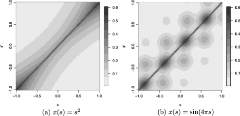
Figure 1: Covariance functions for a one-dimensional spatial process with $M=2$, $\operatorname{logit}(w_{2}(s))=x(s)$, $w_{1}(s)=1-w_{2}(s)$, $K_{1}(s-s^{\prime})=\exp(-|s-s^{\prime}|/0.02)$, and $K_{2}(s-s^{\prime})=\exp(-|s-s^{\prime}|/0.50)$.

There is confounding in (4) between the scale of the weights $w_{j}$ and covariances $K_{j}$, since multiplying the weights by the constant $c>0$ and dividing the standard deviation of $K_{j}$ by $c$ gives the same covariance. Therefore, for identification purposes we restrict the squared weights for each observation to sum to one, $\sum_{j=1}^{M}w_{j}[\mathbf{x}(\mathbf{s},t)]^{2}=1$. Also, allowing the weights to be negative would result in a negative spatiotemporal covariance if $w_{j}[\mathbf{x}(\mathbf{s},t)]>0$ and $w_{j}[\mathbf{x}(\mathbf{s}^{\prime},t^{\prime})]<0$. In some situations this may be desirable, however, we elect to restrict $w_{j}[\mathbf{x}(\mathbf{s},t)]>0$ to ensure a positive spatiotemporal covariance. Section 4 discusses weight selection in further detail.

An important consequence of the covariance construction in (3) is that values of the process at two sites are uncorrelated unless at least one of the $M$ weight functions is positive at both sites. Therefore, unlike other nonstationary covariance models [e.g., Sampson and Guttorp (1992) and Higdon, Swall and Kern (1999)], it may be difficult to separate strength of dependence from severity of nonstationarity. For example, if $M=2$, $w_{1}(\mathbf{s}_{1})=w_{2}(\mathbf{s}_{2})=1$, and $w_{2}(\mathbf{s}_{1})=w_{1}(\mathbf{s}_{2})=0$, then not only is the covariance near $\mathbf{s}_{1}$ different than the covariance near $\mathbf{s}_{2}$, but $\mu(\mathbf{s}_{1})$ and $\mu(\mathbf{s}_{2})$ are necessarily uncorrelated. If this is deemed undesirable for a particular application, one alternative would be to allow for dependence between the latent $\theta_{j}$ using a multivariate spatial model. Another option would be to use only covariates in the weights that have larger spatial range (perhaps pre-smoothed covariates) than the latent $\theta_{j}$ processes, in which case this scenario is less likely. Section 3.2 provides further discussion about the relative roles of the spatial range of the latent and covariate processes.

This covariance model has interesting connections with other commonly used spatial models. For example, if we consider purely spatial data, as mentioned in Section 1, taking the weights to be kernel functions of the spatial location alone, that is, $w_{j}[\mathbf{x}(\mathbf{s})]=w_{j}(\mathbf{s})$, gives the nonstationary spatial model of Fuentes (2002). By modeling the weights as functions of the covariates, it may be possible to explain nonstationarity with fewer terms, giving a more concise and interpretable model. Also, with $M=p$ and $w_{j}[\mathbf{x}(\mathbf{s})]=x_{j}(\mathbf{s})$ for $j=1,\ldots,p$, we obtain the spatially-varying coefficient model of Gelfand et al. (2003). In this model $\theta_{j}(\mathbf{s})$ represents the effect of the $j$th covariate at location $\mathbf{s}$. The motivation for the spatially-varying coefficients model is to study local effects of covariates on the mean response. In contrast, our objective is to model the covariance. For example, in a situation with $p=20$ covariates it may be sufficient to describe the spatial covariance using $M=2$ stationary processes where conditions that favor the two covariance functions are described by weights $w_{1}$ and $w_{2}$ that depend on all $p$ covariates. Therefore, to provide an adequate description of the covariance, we assume the weights are random functions of unknown parameters that describe environmental conditions (see Section 4) rather than taking the weights to be the covariates themselves. Finally, setting the weights $w_{j}$ to be constant in time and the latent processes $\theta_{j}$ to be constant over space gives the spatial dynamic factor model of Lopes, Salazar and Gamerman (2008). Our model differs from this approach since our weights (loadings) are functions of spatial covariates rather than purely stochastic spatial processes.

3 Properties of the covariance model

In this section we discuss some properties of the proposed model in (3) and the spatiotemporal covariance function. For example, it is clear that even if the individual covariances $K_{j}$ are separable, stationary and isotropic, the resulting covariance (4) is in general nonseparable, nonstationary and anisotropic. Below we discuss other properties of the covariance model.

3.1 Monotonicity of the spatial covariance function

As shown in Figure 1, the covariance function can be a nonmonotonic function of spatial distance, even if the underlying covariances $K_{j}$ are decreasing. Intuitively, this occurs only if the spatial range of the covariates is small relative to the spatial range of the covariance functions $K_{j}$. More formally, assuming $\mathbf{s}\in\mathcal{R}$ and the $w_{j}$ and each component of $\mathbf{x}$ are differentiable, then for any $h>0$

$$\frac{\partial\operatorname{Cov}(\mu(\mathbf{s}),\mu(\mathbf{s}+h)|\mathbf{x})}{\partial h}$$

(5)

$$\qquad=\sum_{j=1}^{M}w_{j}(\mathbf{x}[s])w_{j}(\mathbf{x}[s+h])K_{j}(h)\biggl{[}\frac{w_{j}^{\prime}(\mathbf{x}[s+h])}{w_{j}(\mathbf{x}[s+h])}+\frac{K_{j}^{\prime}(h)}{K_{j}(h)}\biggr{]},$$

both $w_{j}^{\prime}$ and $K_{j}^{\prime}$ are derivatives with respect to $h$. Therefore, if the weights $w_{j}(\mathbf{x}[s])$ and covariance $K_{j}(h)$ are positive, a sufficient but not necessary condition for a monotonic covariance is that $w_{j}^{\prime}(\mathbf{x}[s+h])/w_{j}(\mathbf{x}[s+h])+K_{j}^{\prime}(h)/K_{j}(h)<0$ for all $j$. The ratios $w_{j}^{\prime}(\mathbf{x}[s])/w_{j}(\mathbf{x}[s])$ and $-K_{j}^{\prime}(h)/K_{j}(h)$ can be interpreted as the elasticity of the weight function (which depends on both the weight function itself and the derivative of the covariate process) and covariance function, respectively. This condition makes the initial statement more precise, in that (3.1) is negative if the elasticity of the weight function is less than the elasticity of the spatial covariance.

In the special case of a powered-exponential covariance model $K_{j}(\mathbf{s},\mathbf{s}+h)=\tau_{j}^{2}\exp(-\rho_{j}h^{\kappa_{j}})$ and exponential weights $w_{j}(\mathbf{x})=\exp(\mathbf{x}^{T}\bolds\alpha_{j})$, where $\bolds\alpha_{j}$ is a vector of coefficients, (3.1) becomes

$$\frac{\partial\operatorname{Cov}(\mu(\mathbf{s}),\mu(\mathbf{s}+h)|\mathbf{x})}{\partial h}$$

(6)

$$\qquad=\sum_{j=1}^{M}w_{j}(\mathbf{x}[s])w_{j}(\mathbf{x}[s+h])K_{j}(h)[\Delta_{x}(\mathbf{s}+h)^{T}\bolds\alpha_{j}-\kappa_{j}\rho_{j}h^{\kappa_{j}-1}],$$

where $\Delta_{x}(\mathbf{s}+h)$ denotes the vector of derivatives of $x(\mathbf{s}+h)$ with respect to $h$. The covariance is decreasing in $h$ if $\Delta_{x}(\mathbf{s}+h)\bolds\alpha_{j}<\kappa_{j}\rho_{j}h^{\kappa_{j}-1}$ for all $j$ and $h$. This shows that it is possible to allow the spatial covariance to depend on covariates but retain monotonicity by restricting the parameters $\bolds\alpha_{j}$, $\kappa_{j}$ and $\rho_{j}$ based on bounds on the covariate process derivatives.

3.2 Smoothness properties of the spatial process

The smoothness properties of a Gaussian process are often quantified in terms of the mean squared continuity of its derivatives. For many spatial processes, including the nonstationary model of Fuentes (2002), the smoothness of their process realizations is well studied [see Banerjee and Gelfand (2003), Banerjee, Gelfand and Sirmans (2003)]. However, our model postulates a more general dependence of the covariance on spatial covariates. Hence, in this section we explore the effect of that dependence on the smoothness properties of the realizations. For notational convenience, we assume a one-dimensional spatial process with $s\in\mathcal{R}$; the results naturally extend to more general direction derivatives by taking $s=\mathbf{u}^{T}\mathbf{s}$ for any unit vector $\mathbf{u}$. We start by assuming the covariates $\mathbf{x}$ are fixed; this assumption will be later relaxed.

Following the arguments of Banerjee and Gelfand (2003), we say that the $k$th derivative (with respect to $s$) of the process $\mu$ (if it exists) is mean square continuous at $s$ if

$$\lim_{h\rightarrow 0}\mathrm{E}\bigl{[}\mu^{(k)}(s)-\mu^{(k)}(s+h)|\mathbf{x}\bigr{]}^{2}=0.$$ (7)

For $k=0$, we can substitute (3) in (7) and get

$$\lim_{h\rightarrow 0}\mathrm{E}[\mu(s)-\mu(s+h)|\mathbf{x}]^{2}$$

$$\qquad=\sum_{j=1}^{M}\lim_{h\rightarrow 0}K_{j}(0)\bigl{(}w_{j}[\mathbf{x}(s+h)]-w_{j}[\mathbf{x}(s)]\bigr{)}^{2}$$ (8)

$$\qquad\quad{}+\sum_{j=1}^{M}\lim_{h\rightarrow 0}2w_{j}[\mathbf{x}(s)]w_{j}[\mathbf{x}(s+h)]\bigl{(}K_{j}(0)-K_{j}(h)\bigr{)},$$

which shows that $\mu$ is mean square continuous if each latent process is mean square continuous [$\lim_{h\rightarrow 0}K_{j}(h)=K_{j}(0)$] and the weights are smooth enough to satisfy $\lim_{h\rightarrow 0}(w_{j}[\mathbf{x}(s+h)]-w_{j}[\mathbf{x}(s)])^{2}=0$ for all $j$, for example, they are continuous functions of the continuous spatial covariates.

In some settings, it may be reasonable to consider $\mathbf{x}$ to be a random process. We extend the discussion of Banerjee and Gelfand (2003) to the case when the weights are functions of stochastic covariates. In this case, to study the smoothness of $\mu$ requires considering variability in both the latent $\theta_{j}$ as well as the covariates $\mathbf{x}$. The covariates enter the covariance model only through the stochastic weights $W_{j}(s)=w_{j}[\mathbf{x}(s)]$. Taking the expectation with respect to both $\theta_{j}$ and $W_{j}(s)$ gives

$$\lim_{h\rightarrow 0}\mathrm{E}[\mu(s)-\mu(s+h)]^{2}$$

$$\qquad=\sum_{j=1}^{M}\lim_{h\rightarrow 0}K_{j}(0)E_{W_{j}}[W_{j}(s)-W_{j}(s+h)]^{2}$$ (9)

$$\qquad\quad{}+2\sum_{j=1}^{M}\lim_{h\rightarrow 0}\bigl{(}K_{j}(0)-K_{j}(h)\bigr{)}\mathrm{E}_{W_{j}}[W_{j}(s)W_{j}(s+h)].$$

Therefore, under stochastic covariates, the process $\mu$ is mean square continuous if and only if the latent processes $\theta_{j}$ and the weight processes $W_{j}$ are both mean square continuous. It is well known from probability theory that the weight function $W_{j}$ is mean square continuous, for example, if it is bounded and the covariate processes are almost surely continuous. Mean square continuity also follows when $w_{j}$ is Lipschitz continuous of order 1 and the covariate processes are mean square continuous. For example, the logistic weights $w_{j}(\mathbf{x})=\exp(\mathbf{x}^{T}\bolds\alpha_{j})/[1+\exp(\mathbf{x}^{T}\bolds\alpha_{j})]$ are both bounded and Lipschitz continuous of order 1, whereas exponential weights $w_{j}(\mathbf{x})=\exp(\mathbf{x}^{T}\bolds\alpha_{j})$ are not.

These results naturally extend from mean squared continuity to mean square differentiability, and higher order derivatives. Since $\mu(s)$ is the sum of stochastic processes $Z_{j}(s)=W_{j}(s)\theta_{j}(s)$, then $\mu^{(k)}(s)=\sum_{j=1}^{M}Z_{j}^{(k)}(s)$. In particular, for $k=1$ the derivative process at $s$ is

$$\mu^{(1)}(s)=\sum_{j=1}^{M}\theta_{j}^{(1)}(s)W_{j}(s)+\theta_{j}(s)W^{(1)}_{j}(s).$$ (10)

So the process $\mu$ is mean square differentiable if both $W_{j}(s)$ and $\theta_{j}(s)$ are mean square differentiable. Conditions analogous to those outlined above for mean square continuity will assure that the weights are mean square differentiable. More precisely, if the covariate processes $x_{1}(s),\ldots,x_{p}(s)$ are mean square differentiable and the function $w_{j}(\cdot)$ is Lipschitz continuous of order 1, then the resulting process $W_{j}(s)$ is mean square differentiable, and so is $\mu(s)$.

One could go further to study sample path properties and almost sure continuity of the induced spatial process, although the required proofs are generally more difficult than the proofs of mean square properties. If both the weight functions and latent processes are almost surely continuous, then the induced spatial process is also almost surely continuous. Adler (1981) and Kent (1989) provide conditions to verify almost sure continuity for spatial fields.

3.3 Span of the covariance function

The covariance in (4) is quite flexible. For example, consider partitioning the covariate space in $N$ subsets $\mathcal{A}_{1},\ldots,\mathcal{A}_{N}$ and

$$w_{j}[\mathbf{x}(\mathbf{s},t)]=\sum_{i=1}^{N}a_{ji}I\bigl{(}\mathbf{x}(\mathbf{s},t)\in A_{i}\bigr{)}.$$

When $\mathbf{x}(\mathbf{s},t)\in A_{i}$ and $\mathbf{x}(\mathbf{s}^{\prime},t^{\prime})\in A_{k}$, the covariance becomes

$$\operatorname{Cov}(\mu(\mathbf{s},t),\mu(\mathbf{s}^{\prime},t^{\prime})|\mathbf{x})=\sum_{j=1}^{M}a_{ji}a_{jk}K_{j}(\mathbf{s}-\mathbf{s}^{\prime},t-t^{\prime}).$$

Hence, each covariance $K_{j}(\mathbf{s}-\mathbf{s}^{\prime},t-t^{\prime})$ contributes to the mixture differently according to the levels of the covariates. Setting some of the weights $a_{ij}=0$ allows $K_{j}$ to contribute only to the covariance of terms with specific combinations of covariates, for example, both observations have low wind speed and high cloud cover. Also, by setting some of the $a_{ij}<0$, it is possible to specify negative correlation for observations with different levels of the covariate. By increasing $M$ and $N$, this argument shows how the covariate-dependent weights can be used to describe quite general spatiotemporal behavior depending on the covariates.

4 Priors and model-fitting

In this section we describe a convenient specification of the model. For notational convenience, we assume that at each time point observations are taken at spatial locations $\mathbf{s}_{1},\ldots,\mathbf{s}_{N}\in\mathcal{R}^{2}$ and that $t\in\{1,2,\ldots\}$. The overall spatial trend $\delta$ is a Gaussian process with mean zero and spatial covariance $K_{0}^{s}$. We assume that $\delta$’s covariance is stationary, although one could allow $\delta$’s covariance to be nonstationary as well. We assume an autoregressive spatiotemporal model for the latent processes $\theta_{j}$,

$$\theta_{j}(\mathbf{s},t)=\gamma_{j}\theta_{j}(\mathbf{s},t-1)+e_{j}(s,t),$$ (11)

where $\gamma_{j}\in(0,1)$ controls the temporal correlation and the $\mathbf{e}_{jt}=[e_{j}(\mathbf{s}_{1},t),\ldots,\allowbreak e_{j}(\mathbf{s}_{N},t)]$ are independent (over $j$ and $t$) spatial processes with mean zero and spatial covariance $K_{j}^{s}$. We use exponential covariance functions for $K_{j}^{s}$, $j=0,\ldots,M$. We note that although this is a relatively simple specification for the temporal component for each latent process, complex temporal covariance structures can emerge from this mixture model. The covariance between subsequent observations at a site is a mixture of $M$ autoregressive covariances that varies with space and time according to the covariates. This approach could be very useful for modeling hourly ozone which is generally low and steady at night, and high and volatile in the day, which could be fit by including hour of the day as a covariate in the weights.

As mentioned in Section 2, there is confounding in (4) between the scale of the weights $w_{j}$ and covariances $K_{j}$. Therefore, for identification purposes we restrict the squared weights for each observation to sum to one, $\sum_{j=1}^{M}w_{j}[\mathbf{x}(\mathbf{s},t)]^{2}=1$. Although there are other possibilities, we assume the weights have the multinomial logistic form

$$w_{j}[\mathbf{x}(\mathbf{s},t)]^{2}=\frac{\exp{(\mathbf{x}(\mathbf{s},t)^{T}\bolds\alpha_{j})}}{\sum_{l=1}^{M}\exp{(\mathbf{x}(\mathbf{s},t)^{T}\bolds\alpha_{l})}},$$ (12)

where $\bolds\alpha_{1},\ldots,\bolds\alpha_{M}$ are vectors of regression coefficients that control the effects of the covariates on the covariance. For these weights setting $M=1$ gives $w_{1}[\mathbf{x}(\mathbf{s},t)]=1$ and the model is stationary with covariance $K_{1}$. The choice of logistic weights also ensures mean square continuity of the process realizations, as outlined in Section 3. For identification purposes, we fix $\bolds\alpha_{1}=0$, as is customary in logistic regression.

The priors for the hyperparameters are uninformative. We use $\mathrm{N}(0,10^{2})$ priors for the elements of $\bolds\beta$ and $\bolds\alpha_{j}$. The covariance parameters have priors $\sigma^{-2},\tau_{j}^{-2}\stackrel{{\scriptstyle\mathrm{i.i.d.}}}{{\sim}}\operatorname{Gamma}(0.1,0.1)$, and $\gamma_{j}\sim\operatorname{Unif}(0,1)$. Also, we take $K^{s}_{j}(\|h_{s}\|)=\exp(-\|h_{s}\|/\rho_{j})$, where $h_{s}$ is the distance between points after a Mercator projection, scaled to correspond roughly to distance in kilometers, and $\rho_{j}\sim\operatorname{Unif}(0,2\mbox{,}000)$.

The covariance and the effect of an individual covariate on the covariance in (4) are rather obscure. This is due to the label-switching problem, that is, the labels of the processes are arbitrary: for example, $\theta_{1}$ may correspond to a high variance process for some MCMC iterations and to a small variance process for others, making inference on individual parameters difficult. One remedy for the label-switching problem is to introduce constraints, perhaps, $\operatorname{Var}(\theta_{1})<\cdots<\operatorname{Var}(\theta_{M})$. However, ordering constraints on complex functions such as spatiotemporal covariance functions is not straightforward. Therefore, rather than summarizing the individual parameters in the model, we summarize the entire covariance function for different combinations of covariates. A simple way to summarize the effect of the $k$th covariate is in terms of the posterior of the ratio of the covariance of two observations with $x_{k}=2$ (standard deviation units above the mean) compared to the covariance of two observations with $x_{k}=0$, assuming all other covariates are fixed at zero (their mean). That is,

$$\Delta_{k}(h_{s},h_{t})=\frac{\sum_{j=1}^{M}(({\exp(\alpha_{j1}+\alpha_{jk})})/({\sum_{l=1}^{M}\exp(\alpha_{l1}+\alpha_{lk})}))K_{j}(h_{s},h_{t})}{\sum_{j=1}^{M}(({\exp(\alpha_{j1})})/({\sum_{l=1}^{M}\exp(\alpha_{l1})}))K_{j}(h_{s},h_{t})},$$ (13)

where $\alpha_{jk}$ is the $k$th element of $\bolds\alpha_{j}$ and $K_{j}(h_{s},h_{t})=K_{j}^{s}(\|h_{s}\|)\gamma_{j}^{|h_{t}|}$. We also inspect the ratio of correlations ${\tilde{\Delta}}_{k}(h_{s},h_{t})=\Delta_{k}(h_{s},h_{t})/\Delta_{k}(0,0)$. We consider a covariate to have a significant effect on the variance if the posterior interval for $\Delta_{k}(0,0)$ excludes one. Similarly, we consider a covariate to have a significant effect on the spatial (temporal) correlation if the posterior interval for ${\tilde{\Delta}}_{k}(h_{s},0)$ [${\tilde{\Delta}}_{k}(0,h_{t})$] excludes one.

Finally, we discuss how to select the number of terms, $M$. One approach would be to model $M$ as unknown and average over model space using reversible jump MCMC. Lopes, Salazar and Gamerman (2008), Salazar, Lopes and Gamerman (2011) use reversible jump MCMC to select the number of factors in a latent spatial factor model. However, this approach is likely to pose computational challenges for large spatiotemporal data sets. Therefore, we select the number of terms using cross-validation and assume $M$ is fixed in the final analysis. For cross-validation, we randomly (across space and time) split the data into training ($n=63$,881) and testing ($N=3$,367) sets. We fit the model on the training data and compute the posterior predictive distribution for each test set observation. We then compute the mean squared error $\mathrm{MSE}=\sum_{i}(Y_{i}-{\bar{Y}}_{i})^{2}/N$ and mean absolute deviation $\mathrm{MAD}=\sum_{i}(Y_{i}-{\tilde{Y}}_{i})^{2}/N$, where the sum is over the $N$ test set observations, ${\bar{Y}}_{i}$ is the posterior mean, and ${\tilde{Y}}_{i}$ is the posterior median. We also compute the mean (over the test set observations) of the posterior predictive variances (“AVE VAR”), the median of the posterior predictive standard deviations (“MED SD”) and the coverage probability of 95% prediction intervals.

5 Computational details

We implement the model in R (http://www. r-project.org/). Though implementation in WinBUGS (http://www.mrc- bsu.cam.ac.uk/bugs/) would also be straightforward, run times might be long for large data sets. We update $\bolds\theta_{jt}=[\theta_{j}(\mathbf{s}_{1},t),\ldots,\theta_{j}(\mathbf{s}_{N},t)]$, $\bolds\beta$, $\sigma^{2}$ and $\gamma_{j}$, which have conjugate full conditionals, via Gibbs sampling, and we update $\alpha_{jk}$, $\rho_{j}$ and $\nu_{j}$ using Metropolis–Hastings sampling with a Gaussian candidate distribution tuned to give acceptance probability around 0.4.

Sampling using the dynamic spatial model in (11) allows us to update the $\bolds\theta_{jt}$ as a block and avoid inverting large matrices. The alternative of sampling after marginalizing out the latent $\bolds\theta_{jt}$ would require computing the entire spatiotemporal covariance with elements given by (4), which would likely give better mixing for small to moderate data sets. For our large data set, however, matrix computations of this size are not feasible.

We monitor convergence with trace and autocorrelation plots for several representative parameters. Monitoring convergence is challenging for this model since the labels of the latent terms may switch during MCMC sampling: exchanging $\bolds\alpha_{1}$, $\rho_{1}$, $\nu_{1}$ and $\gamma_{1}$, for example, with $\bolds\alpha_{2}$, $\rho_{2}$, $\nu_{2}$ and $\gamma_{2}$, does not affect the covariance in (4). Rather than monitoring convergence for these parameters individually, we therefore monitor convergence of the covariance (4) at several lags and of the spatiotemporal effect $\mu(\mathbf{s},t)$ for several spatiotemporal locations. For the application in Section 6 we generate 20,000 samples, discarding the first 10,000 as burn-in. For the exponential covariances considered here this appears to be sufficient; however, for smoother processes, such as those induced by the squared exponential covariance, 20,000 iterations may not be sufficient.

6 Application to southeastern US daily ozone

To illustrate our spatiotemporal covariance model, we analyze ozone in the southeast US. The primary National Ambient Air Quality Standard (NAAQS) for ozone requires the three-year average of the annual fourth-highest daily maximum 8-hour daily average concentration to fall beneath 75 parts per billion (ppb) [CFR (2008), pages 16436–16514]. Our response variable is thus the square root—to ensure Gaussianity—of the daily “8-hour ozone” metric. We focus on the $89$ sites in North Carolina, South Carolina and Georgia shown in Figure 2. This geographically heterogeneous region transitions from the flat, low-altitude coastal plains in the east, to the gentle, rolling hills of the piedmont, to mountains in the northwest, with a handful of urban islands buffered by suburbs that give way to rural tracts. Since summertime ozone concentrations are highest, and therefore most relevant for attainment determination, we extract daily 8-hour ozone concentrations, longitude, latitude, elevation and site classification (urban, suburban or rural) for June–August, 1997–2005 ($6444/73$,$692=8.7$% missing) from the US EPA Air Quality System (AQS) database, available via the Air Explorer web tool (http:// www.epa.gov/airexplorer/index.htm).

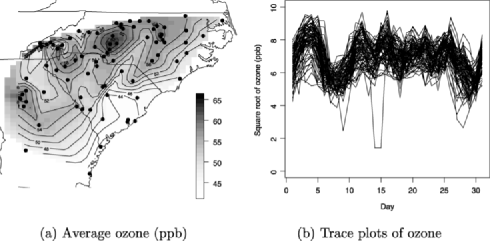
Figure 2: Plots of square root ozone (pbb). Panel (a) plots the average for each station (the stations are marked with points) and panel (b) gives trace plots for each station in August 2005 (Day 1 is August 1, 2005).

We obtain daily average temperature and daily maximum wind speed from the National Climatic Data Center (NCDC) Global Summary of the Day and daily average cloud cover from the NCDC National Solar Radiation database. Since meteorological and ozone data are not observed at the same locations, for each day we predict each meteorological variable at ozone observation sites using spatial Kriging implemented in SAS V9.1 Proc MIXED with an exponential covariance function. Though Li, Tang and Lin (2009) show that ignoring uncertainty when using spatial predictions of covariates is not without consequence, accounting for that uncertainty is nontrivial. Since our current focus is the development of the covariate-dependent covariance model, we treat these predictions as fixed.

Covariates $\mathbf{x}(\mathbf{s},t)$ in the mean trend include the continuous variables temperature, wind speed, cloud cover, elevation, longitude, latitude and a linear trend in year, each standardized to have mean zero and variance one, and we include two indicator variables identifying a station as urban or rural, leaving suburban as the baseline. We have no detailed land-use covariates as in Paciorek et al. (2009), however, which would likely improve fine-scale prediction. We consider all two-way interactions between the three meteorological variables and quadratic effects of the meteorological variables. The covariance is modeled as a function of only the main effects of these covariates.

6.1 Empirical variogram analysis

We begin studying the data by analyzing the spatial variogram, defined as $\gamma(h)=E([r(\mathbf{s},t)-r(\mathbf{s}+h\mathbf{u},t)]^{2})$, where $r(\mathbf{s},t)$ is the residual after accounting for the mean trend and $\mathbf{u}$ is a unit vector. Though there is evidence that regression coefficient estimation can be affected by disregarding spatial correlation [Reich, Hodges and Zadnik (2006), Wakefield (2007), Paciorek (2010)], for simplicity we use ordinary least squares, pooled over all observations, to estimate the mean trend. We estimate the variogram as the mean squared difference between all pairs of observations in a bin $D_{h}$, that is,

$${\hat{\gamma}}(h)=\frac{1}{|D_{h}|}\sum_{t}\sum_{(\mathbf{s},\mathbf{s}^{\prime})\in D_{h}}[r(\mathbf{s},t)-r(\mathbf{s}^{\prime},t)]^{2},$$ (14)

where $D_{h}$ is the set of pairs of points on the same day with $\|\mathbf{s}-\mathbf{s}^{\prime}\|\in(h-\epsilon,h+\epsilon)$ and $|D_{h}|$ is the cardinality of $D_{h}$.

Figure 3: Sample variograms for the ozone data by cloud cover. The data are plotted separately for pairs of observations with both (“Low–Low”), one (“Low–High”) and neither (“High–High”) members of the pair with cloud cover below the median cloud cover. Panel (b) plots the ratio of curves in (a), panel (c) uses log-transformed, rather than square-root-transformed data, and panel (d) standardizes the residuals by the daily sample standard deviation.

Figure 4: Sample variograms for the ozone data by wind speed. The data are plotted separately for pairs of observations with both (“Low–Low”), one (“Low–High”) and neither (“High–High”) members of the pair with wind speed below the median wind speed. Panel (b) plots the ratio of curves in (a), panel (c) uses log-transformed, rather than square-root-transformed data, and panel (d) standardizes the residuals by the daily sample standard deviation.

To explore the effects of each of the covariates on the spatial covariance, we compute individual variograms for three categories of site pairings. In the “low–low” category, both sites have values of the covariate below the sample median for the covariate; in the “high–high” category, both have values above the median; and in the “low–high” category, one has a value below, and the other above, the median. Such variograms for cloud cover and wind speed are given in Figures 3 and 4, respectively.

In Figure 3(a), the variogram is lowest for pairs of observations for which both sites have high cloud cover, higher when both sites have low cloud cover, and highest when one site has low and the other high cloud cover. Solar radiation is required to turn NO₂ into ozone or to create VOC’s that turn NO into NO₂. Therefore, under high cloud cover conditions, ozone levels would be expected to drop close to background levels (a long-term equilibrium that would exist in the absence of local emissions), which would be homogeneous over a region of this size. Two sites for which cloud cover is low would be expected to be less similar to each other than would two sites that both have high cloud cover because the production of ozone via solar radiation is now dependent on the spatially-varying precursors. For example, areas very close to major sources of NOx (power plants and urban centers on workdays) would have low ozone due to NOx scavenging, and moving downwind from these sources, ozone would increase and then decrease. Finally, based on the explanation above, it is clear that if one site has high cloud cover, so that ozone production is minimal, and the other has low cloud cover, so that ozone production is rampant, they would have very dissimilar ozone values, so that the variogram would be highest for the low–high category.

Wind speed does not generally affect the chemical reactions that create or destroy ozone, but it does transport ozone and its precursors. One would expect that within smaller subregions with higher wind speeds, distance is effectively shortened so that spatial correlation would be higher, and two sites in the “high–high” category would have lower variogram, followed by those with “low–high,” then “low–low,” as we see in Figures 4(a) and 4(b) for spatial lags below 250 km. The ordering of the categories is reversed for larger spatial lags, where transport is less relevant.

In addition to computing these variograms for our square root ozone response, we compute the variograms using residuals from a regression on the log, rather than square root, of ozone, and the variogram of standardized residuals, that is, $r^{*}(\mathbf{s},t)=r(\mathbf{s},t)/s_{t}$, where $s_{t}$ is the sample standard deviation of the residuals for day $t$. The variograms are affected more by the log transformation than by standardizing. The same general patterns remain after standardizing, but new ones emerge after a log transformation. For example, the ordering of the variograms for cloudy and sunny days switches after a log transformation in Figure 3. The patterns of the log-transformed responses also indicate covariate-dependent covariance, so it appears that the transformation is important, but does not resolve nonstationarity.

6.2 Results

We fit five versions of the model, with the number of mixture components varying from $M=1$ to $5$. We withheld 5% of the observations (3,687 observations), selected randomly across space and time. Table 1 compares for predictions of square root ozone for this validation set. For all models, the prediction intervals have coverage greater than 0.95. The five-component model minimizes all measures of prediction error and variance. The ratio of mean squared error for the five-component model to that of the stationary one-component model is $0.179/0.189=0.947$, and the corresponding ratio of average prediction variances is $0.167/0.183=0.913$. The nonstationary covariance thus gives a modest improvement in prediction accuracy and uncertainty quantification. We also tried higher values of $M$ and found slight improvements in prediction, but elected to proceed with $M=5$ for model simplicity.

Table 1: Validation set results. The summaries are mean squared error (MSE), median absolute deviation (MAD), mean posterior predictive variance (AVE VAR), median posterior predictive standard deviation (MED SD) and coverage probability of 95% intervals (COV). All values are multiplied by 100

	$\bolds{M}$
	1	2	3	4	5
MSE	18.9	18.6	18.3	18.2	17.9
MAD	23.5	22.7	22.2	22.0	21.4
AVE VAR	18.3	17.0	16.7	16.4	16.7
MED SD	41.9	40.0	39.2	38.8	38.2
COV	95.7	95.5	95.3	95.3	95.2

The largest effect of nonstationary is in the measures of prediction uncertainty. Figure 5 plots the prediction standard deviation for the observations in the validation set for the stationary model with $M=1$ and the nonstationary model with $M=5$. The standard deviation is smaller for the nonstationary model for 72% of the observations, and varies far more across observations for the nonstationary model (roughly from 0.25 to 0.80) compared to the stationary model (roughly 0.35 to 0.65). To show that the conditional coverage remains valid for both models, we separated the validation set into five equally sized groups based on the ratio of standard deviations from the models with $M=5$ to $M=1$. The coverage of 95% intervals in these five groups (from smallest to largest relative variance) is 0.97, 0.97, 0.96, 0.96 and 0.93 for the stationary model and 0.93, 0.96, 0.94, 0.97 and 0.96 for the nonstationary model.

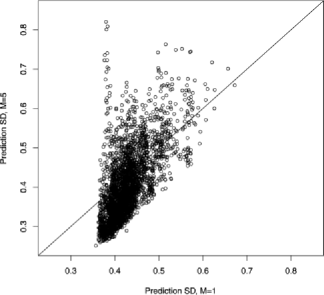
Figure 5: Posterior predictive standard deviation for the observations in the validation set for the stationary model with $M=1$ compared to the nonstationary model with $M=5$.

Table 2: Summary of the model with $M=5$ components. The remaining columns give the posterior means (95% intervals) for the mean effects $\beta_{k}$, the relative variance $(\Delta_{k}(0,0))$, the relative spatial correlation at lag 100 km $({\tilde{\Delta}}_{k}(100,0))$, and the relative temporal correlation at lag 2 days $({\tilde{\Delta}}_{k}(0,2))$. $\beta_{k}$, $\Delta_{k}(0,0)$, ${\tilde{\Delta}}_{k}(100,0)$, and ${\tilde{\Delta}}_{k}(0,2)$ are scaled to represent the effect of a two standard deviation increase in the predictor

	Mean	Variance	Spatial cor.	Temporal cor.
	$\bolds{\beta_{k}}$	$\bolds{\Delta_{k}(0,0)}$	$\bolds{{\tilde{\Delta}}_{k}(100,0)}$	$\bolds{{\tilde{\Delta}}_{k}(0,2)}$
Temperature (F)	0.333 ($0.331,0.358$)	1.09 ($1.06,1.12$)	0.88 ($0.86,0.90$)	1.09 ($1.03,1.16$)
Wind speed (m/s)	$-$0.028 ($-0.037,-0.019$)	0.96 ($0.94,0.97$)	1.05 ($1.04,1.06$)	0.97 ($0.94,1.00$)
Cloud cover (%)	$-$0.154 ($-0.173,-0.134$)	1.12 ($1.07,1.17$)	1.05 ($1.03,1.06$)	0.57 ($0.51,0.64$)
Elevation (ft)	0.115 ($0.078,0.183$)	0.98 ($0.96,1.01$)	1.10 ($1.09,1.11$)	1.30 ($1.24,1.37$)
Urban	0.007 ($-0.020,0.035$)	1.00 ($0.98,1.02$)	0.95 ($0.93,0.96$)	0.99 ($0.96,1.02$)
Rural	0.045 ($0.010,0.066$)	0.57 ($0.43,0.77$)	0.94 ($0.90,0.97$)	1.17 ($1.02,1.37$)
Year	0.004 ($-0.001,0.008$)	1.01 ($1.00,1.02$)	1.03 ($1.02,1.03$)	0.95 ($0.93,0.97$)
Longitude	0.096 ($0.018,0.187$)	0.99 ($0.94,1.03$)	1.12 ($1.10,1.13$)	1.53 ($1.43,1.62$)
Latitude	0.185 ($0.089,0.251$)	0.70 ($0.67,0.74$)	1.05 ($1.03,1.07$)	0.48 ($0.40,0.55$)
Temp2	0.023 ($0.014,0.032$)	–	–	–
WS2	0.004 ($0.002,0.005$)	–	–	–
CC2	$-$0.020 ($-0.029,-0.010$)	–	–	–
Temp${}\times{}$WS	$-$0.005 ($-0.013,0.003$)	–	–	–
Temp${}\times{}$CC	0.055 ($0.044,0.068$)	–	–	–
WS${}\times{}$CC	0.004 ($-0.003,0.012$)	–	–	–

Table 2 and Figure 6 summarize the covariate effects on the mean and spatiotemporal correlation for the full data set with $M=5$. The mean trend accounts for most of the variability in square root ozone: though the sample variance of the observations is 1.61 ppb, the posterior means of the spatial effects $\delta(\mathbf{s})$ have variance 0.09 ppb. The statistical significance of the linear and quadratic temperature terms and the positive effect of temperature on variance are consistent with findings of Nail, Hughes-Oliver and Monahan (2010) and others that ozone concentration is a monotone increasing nonlinear function of temperature, and ozone variance increases with the mean. It is reasonable that spatial correlation decreases as temperature increases due to the fact that when the solar radiation is conducive to the chemical reactions that produce ozone, that production is a function of local emissions, and highly nonlinear in NOx emissions, which vary over space. Similarly, it is reasonable that spatial correlation at short spatial lags increases with wind speed because wind facilitates transport of ozone and its precursors.

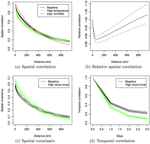
Figure 6: Posterior mean (thick lines) and 95% intervals (thin lines) of the spatiotemporal correlation (4) for various combinations of the covariates. “Baseline” assumes that all covariates are zero (the mean after standardization) for both observations. The other plots assume that all covariates are zero with the exception of one covariate, which equals two standard deviation units above the mean. Panel (b) plots the posterior of ratio of the spatial correlations under high temperature and baseline conditions plotted in panel (a). The spatial correlation is plotted as a function of spatial distance $h_{s}$ with temporal distance $h_{t}=0$, and vice versa.

As discussed in Section 6.1, the relationship between cloud cover and ozone is quite complex. We find that cloud cover is negatively associated with the mean and temporal correlation, and positively associated with variance and spatial correlation. As expected, mean ozone decreases and spatial correlation increases with cloud cover since ozone levels drop near low, heterogenous background levels in the absence of solar radiation. A possible explanation for low variance and high temporal autocorrelation for sunny days is the common southeastern summertime meteorological regime called the “Bermuda high,” which is characterized by sunny skies and high atmospheric pressure indicative of a lower atmospheric boundary layer. The lowered ceiling combined with low wind speed effectively reduce the volume in which emissions interact, which, combined with high solar radiation, creates a simmering cauldron of ozone production. Because the Bermuda high persists over several days and spans regions greater than or equal to the size of our spatial domain, ozone production is high everywhere, so that the variability is lower and the temporal correlation is higher.

Figure 6 plots the estimated spatial and temporal covariance for several combinations of the covariates. Figures 6(a) and 6(b) show that the estimated spatial correlation is lower for spatial lags less than 100 km for hot days, and that temperature is less relevant at larger distances. This plot also shows the mixture of exponential correlation functions gives a correlation that is significantly different than a simple exponential correlation. The mixture correlation function drops more quickly near the origin and has a heavier tail than an exponential correlation. Cloud cover also affects both the spatial covariance and temporal autocorrelation. Figure 6(c) shows that the variance is higher on cloudy days, but the covariance has smaller spatial range. Also, the temporal correlation in Figure 6(d) is higher for lags one, two and three for sunny days.

Figure 7 compares the posterior mean of the stationary one-component model to that of the nonstationary five-component model,

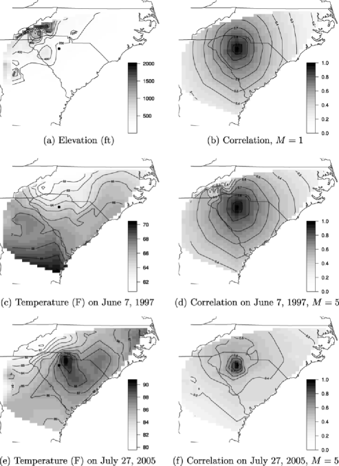
Figure 7: Data and spatial correlation estimates for two days for stationary ($M=1$) and nonstationary ($M=5$) models. Panels (b), (d) and (f) plot the posterior mean of the correlation between the point marked with a dot and the remaining sites.

and shows the relationship between the spatial covariance of the latter model with temperature and elevation. Figure 7(b) shows the exponential decay in correlation with increasing distance from the marked site for the stationary model; this correlation function is the same for the two days under consideration, June 7, 1997, and July 27, 2005, which have the minimum and maximum temperatures at the marked site. The temperature contours for those days are plotted in Figures 7(c) and 7(e), and elevation contours are plotted in Figure 7(a). The spatial correlation contours in the northwest of Figure 7(d) show the negative effect of elevation on spatial correlation. The July 27, 2005 position of the maximum temperature peak over the marked site clearly shows the effect of temperature on the steepness of the decline in correlation at short versus long lags seen earlier in Figure 6(a). The effect of elevation on correlation is dwarfed by the effect of temperature, likely due to the positioning of the temperature peak over the marked site combined with the magnitude of the temperature at that peak.

7 Discussion

In this paper we present a class of spatiotemporal covariance functions that allows the covariance to depend on environmental conditions described by known covariates. Although fitting this, and other sophisticated spatiotemporal models, likely requires expertise in spatial statistics and computing methods, the method produces interpretable summaries of the effect of each covariate on the mean, variance, and spatial and temporal ranges. For the southeastern US ozone data, we find our nonstationary analysis improves prediction error, reduces prediction variance, and achieves the desired coverage probabilities, while identifying several interesting covariate effects on both the mean and covariance.

Our covariance model assumes that all nonstationarity can be explained by the spatial covariates. However, in some cases a more flexible model would be useful. One approach would be to add more pure functions of space and time as covariates in the covariance to capture nonstationarity. An even more flexible model would take the weights to be Gaussian processes, possibly with means that depend on the covariates, to allow the weights to vary smoothly through the spatial domain while still making use of the covariate information.

References

- Adler (1981) {bbook}[mr] \bauthor\bsnmAdler, \bfnmRobert J.\binitsR. J. (\byear1981). \btitleThe Geometry of Random Fields. \bpublisherWiley, \baddressLondon. \bidmr=0611857 \endbibitem
- Banerjee and Gelfand (2003) {barticle}[mr] \bauthor\bsnmBanerjee, \bfnmS.\binitsS. and \bauthor\bsnmGelfand, \bfnmA. E.\binitsA. E. (\byear2003). \btitleOn smoothness properties of spatial processes. \bjournalJ. Multivariate Anal. \bvolume84 \bpages85–100. \biddoi=10.1016/S0047-259X(02)00016-7, issn=0047-259X, mr=1965824 \endbibitem
- Banerjee, Gelfand and Sirmans (2003) {barticle}[mr] \bauthor\bsnmBanerjee, \bfnmSudipto\binitsS., \bauthor\bsnmGelfand, \bfnmAlan E.\binitsA. E. and \bauthor\bsnmSirmans, \bfnmC. F.\binitsC. F. (\byear2003). \btitleDirectional rates of change under spatial process models. \bjournalJ. Amer. Statist. Assoc. \bvolume98 \bpages946–954. \biddoi=10.1198/C16214503000000909, issn=0162-1459, mr=2041483 \endbibitem
- Berrocal, Gelfand and Holland (2010) {barticle}[auto:STB—2011-03-03—12:04:44] \bauthor\bsnmBerrocal, \bfnmV. J.\binitsV. J., \bauthor\bsnmGelfand, \bfnmA. E.\binitsA. E. and \bauthor\bsnmHolland, \bfnmD. M.\binitsD. M. (\byear2010). \btitleA spatio-temporal downscaler for output from numerical models. \bjournalJ. Agric. Biol. Environ. Stat. \bvolume15 \bpages176–197. \endbibitem
- Carroll et al. (1997) {barticle}[auto:STB—2011-03-03—12:04:44] \bauthor\bsnmCarroll, \bfnmR.\binitsR., \bauthor\bsnmChen, \bfnmR.\binitsR., \bauthor\bsnmGeorge, \bfnmE.\binitsE., \bauthor\bsnmLi, \bfnmT.\binitsT., \bauthor\bsnmNewton, \bfnmH.\binitsH., \bauthor\bsnmSchmiediche, \bfnmH.\binitsH. and \bauthor\bsnmWang, \bfnmN.\binitsN. (\byear1997). \btitleOzone exposure and population density in Harris County, Texas. \bjournalJ. Amer. Statist. Assoc. \bvolume92 \bpages392–404. \endbibitem
- CFR (2008) {bmisc}[auto:STB—2011-03-03—12:04:44] \borganizationCFR (\byear2008). \bhowpublished40 CFR Parts 50 and 58, National Ambient Air Quality Standards for Ozone, Final rule. \endbibitem