Evolution of the Symbiotic Nova PU Vul – Outbursting White Dwarf, Nebulae, and Pulsating Red Giant Companion

Abstract

We present a composite light-curve model of the symbiotic nova PU Vul (Nova Vulpeculae 1979) that shows a long-lasted flat optical peak followed by a slow decline. Our model light-curve consists of three components of emission, i.e., an outbursting white dwarf (WD), its M-giant companion, and nebulae. The WD component dominates in the flat peak while the nebulae dominate after the photospheric temperature of the WD rises to $\log T$ (K) $\gtrsim 4.5$, suggesting its WD origin. We analyze the 1980 and 1994 eclipses to be total eclipses of the WD occulted by the pulsating M-giant companion with two sources of the nebular emission; one is an unocculted nebula of the M-giant’s cool-wind origin and the other is a partially occulted nebula associated to the WD. We confirmed our theoretical outburst model of PU Vul by new observational estimates, that spanned 32 yr, of the temperature and radius. Also our eclipse analysis confirmed that the WD photosphere decreased by two orders of magnitude between the 1980 and 1994 eclipses. We obtain the reddening $E(B-V)\sim 0.3$ and distance to PU Vul $d\sim 4.7$ kpc. We interpret the recent recovery of brightness in terms of eclipse of the hot nebula surrounding the WD, suggesting that hydrogen burning is still going on. To detect supersoft X-rays, we recommend X-ray observations around June 2014 when absorption by neutral hydrogen is minimum.

1. Introduction

Symbiotic novae are thermonuclear runaway phenomena occurring on white dwarfs (WDs) in binary systems that consist of a WD and a red giant (RG). Symbiotic novae can be divided into two subgroups according to their spectral evolutions. The first group exhibit a long (several years) “supergiant phase,” resembling an A-F supergiant when the star underwent an outburst. In the second group, a nebular phase begins almost immediately after the optical maximum, and a “supergiant phase,” if there is, has a very short duration (Mürset & Nussbaumer, 1994). The first subgroup include AG Peg, RT Ser, RR Tel, and PU Vul. The second subgroup include V1016 Cyg, HBV 475, and HM Sge. It is, however, still unknown the reason why this difference arises. Due to very long evolution-timescales (one to several tens of years or more) it is not easy to obtain observational data of a whole period of the outbursts, such as dense and continuous photometric, spectroscopic, and multi-wavelength observations including UV and X-ray. Under these circumstances, it has been difficult to study symbiotic novae quantitatively compared with classical novae.

Among symbiotic novae, PU Vul is a rare exception. It is an eclipsing binary of the orbital period $\sim 4900$ days (13.4 yr) (Kolotilov et al., 1995; Nussbaumer & Vogel, 1996; Garnavich, 1996; Shugarov et al., 2011). During eclipses, different emission components are occulted differently. This offers a good chance for quantitative study. PU Vul outbursted in 1979 and we have dense optical spectroscopic/photometric data as well as IUE/HST UV observations. Recently, Kato et al. (2011) first presented a theoretical model of PU Vul that reproduces the optical flat peak as well as the UV light curve, and estimated the WD mass ($\sim 0.6~{}M_{\odot}$). Their model is, however, only for the light curve of the outbursting component (WD) and the other emission components were neglected.

This paper presents a comprehensive model of emission components of the WD, RG, and nebulae, based on new estimates of the temperature and radius of the hot component (WD), as well as the cool component (RG) derived from the two eclipses (1980 and 1994). Section 2 briefly introduces our evolution model of PU Vul. Using our theoretical light curves, we constrain the extinction and distance to PU Vul in Section 3. Section 4 compares our theoretical light curves with our new observational estimates of temperature and radius of the WD. In Section 5, we analyze light curves of the two eclipses and obtain the binary parameters as well as the brightnesses of the RG and nebulae. Using these values, we construct a composite light curve model of PU Vul in Section 6. Discussion and conclusions follow in Sections 7 and 8.

2. Model of WD component

2.1. Evolution of Nova Outbursts

A nova is a thermonuclear runaway event on a WD. After the hydrogen shell flash sets in, the envelope on the WD expands to a giant size. After it reaches the optical peak, the envelope settles down into a steady-state. The optical magnitude decays as the envelope mass decreases while the photospheric temperature rises with time. The decay phase can be followed by a quasi-static sequence (Kato et al., 2011). We solved the equations of hydrostatic balance, continuity, radiative diffusion, and conservation of energy, from the bottom of the hydrogen-rich envelope through the photosphere. The evolution is followed by a sequence of decreasing envelope mass. The time interval $\Delta t$ between two successive solutions is calculated by $\Delta t=\Delta M_{\rm env}/(\dot{M}_{\rm nuc}+\dot{M}_{\rm wind})$, where $\Delta M_{\rm env}$ is the difference between the envelope masses of the two successive solutions, and $\dot{M}_{\rm nuc}$ is the hydrogen nuclear burning rate and $\dot{M}_{\rm wind}$ is the optically-thin wind mass-loss rate (see Equation (24) in Kato & Hachisu, 1994, for more detail). The method and numerical techniques are essentially the same as those in Kato et al. (2011). We used OPAL opacities (Iglesias & Rogers, 1996). The WD radius (the bottom of hydrogen shell-burning) is assumed to be the Chandrasekhar radius. The mixing-length parameter of convection $\alpha$ is assumed to be 1.5 (see Kato & Hachisu (2009) for the dependence of the light curve on $\alpha$). Internal structures of the envelope are essentially the same as those in Figure 7 of Kato et al. (2011). We calculate optical and UV light curves from the blackbody spectrum with the photospheric temperature, $T_{\rm ph}$. To calculate $V$ magnitude, we use the standard Johnson $V$ bandpass and add a bolometric correction of 0.17 mag (see Section 4).

In our model, we simply assume uniform chemical composition of the envelope. PU Vul does not show any CO/Ne enrichment but the overall chemical composition is almost consistent with being solar; slightly subsolar of iron (Belyakina et al., 1984, 1989) and helium overabundance (Andrillat & Houziaux, 1994; Luna & Costa, 2005) are reported. Thus, we assume four different sets of chemical composition ($X$, $Y$, $Z$) by weight for hydrogen, helium, and heavy elements of the envelope as (0.7, 0.29, 0.01), (0.7, 0.28, 0.02) (0.5, 0.49, 0.01), and (0.5, 0.49, 0.006). Here $Z=0.01$ is closer to the recent estimate of heavy element abundance of solar composition ($Z=0.0128$: Grevesse, 2008). The WD mass is assumed to be 0.6 $M_{\odot}$ as listed in Table 1. Model 4 in Table 1 is the same as Model 2 in Kato et al. (2011).

A typical classical nova shows heavy element enrichment (C, O, and Ne) in its ejecta, which is interpreted in terms of dredge-up of WD material (Prialnik & Kovetz, 1984, 1995). PU Vul shows no indication of such enhancement in spectra, which suggests that the WD is not eroded during and before the outburst. The theoretical model described in Kato et al. (2011) showed that only a small part of the accreted matter was lost in the optically-thin wind, and the rest was burned to helium due to hydrogen nuclear burning and accumulated on the WD. Therefore, the WD develops a helium layer underneath the newly accreted material. In the next outburst, a part of the helium layer will possibly be dredged up and mixed into the upper hydrogen layer. In such a case the envelope will become helium-rich like in Models 3 and 4 in Table 1.

There are observational evidences of wind mass-loss from WDs in some symbiotic stars. For PU Vul, Tomov et al. (1991) found broad emission wings in H I, He I, He II and N IV lines as well as violet-shifted P Cygni type absorption components in H I and He I lines in the optical spectra taken in 1990-91, which they attributed to the hot component winds. Sion et al. (1993) discussed the onset of Wolf-Rayet type wind outflowing from the hot component based on the IUE high resolution spectra of 1989-1991, and estimated an upper limit of $\dot{M}_{\rm wind}\lesssim 10^{-5}~{}M_{\odot}$ yr^-1. For AG Peg, the outburst lasted about 150 yr, which suggests a low mass WD with no optically-thick winds. The wind mass-loss rate from the hot component was estimated to be of the order of $10^{-7}~{}M_{\odot}$ yr^-1 (Vogel & Nussbaumer, 1994) and $10^{-6}~{}M_{\odot}$ yr^-1 (Kenyon et al., 1993). The intensity of the wind diminished in step with the hot component luminosity during the decline of the outburst. For AE Ara, the wind mass loss rate is estimated to be a few times $10^{-8}$ – $10^{-7}M_{\odot}$ yr^-1 and the WD mass to be $M_{\rm h}\sin~{}i\sim 0.4~{}M_{\odot}$ (Mikołajewska et al., 2003).

With such poor information on mass-loss rates, we simply assume that an optically-thin wind begins to blow when the photospheric temperature rises to $\log T_{\rm ph}$ (K) $\sim 4.0$ and the wind continues until $\log T_{\rm ph}$ (K) $\sim 5.05$ at various rates listed in Table 1 (e.g., $\dot{M}_{\rm wind}=5.0\times 10^{-7}M_{\odot}$ yr^-1 for Model 1). After the temperature reaches $\log T_{\rm ph}$ (K) $\sim 5.05$, the wind mass-loss rate drops to $\dot{M}_{\rm wind}\sim 1.0\times 10^{-7}M_{\odot}$ yr^-1.

We cannot accurately determine the WD mass of PU Vul only from our light curve analysis. Kato et al. (2011) obtained a plausible range of the WD mass, 0.5 – 0.72 $M_{\odot}$ corresponding to a reasonable range of the wind mass-loss rates. In the present paper, we adopt an 0.6 $M_{\odot}$ WD as a standard model of PU Vul (see Section 2.2 for more detail).

Table 1Model Parameters

Subject		Model 1	Model 2	Model 3	Model 4	Units
$X$	…	0.7	0.7	0.5	0.5
$Y$	…	0.29	0.28	0.49	0.494
$Z$	…	0.01	0.02	0.01	0.006
WD mass	…	0.6	0.6	0.6	0.6	$M_{\odot}$
$M_{\rm bol}$	…	$-5.44$	$-5.36$	$-5.63$	$-5.68$	mag
$M_{V,{\rm peak}}$	…	$-5.61$	$-5.53$	$-5.80$	$-5.85$	mag
$L_{\rm peak}$	…	4.6	4.2	5.5	5.7	$10^{37}$erg s-1
maximum radius	…	63	60	61	64	$R_{\odot}$
initial envelope mass	…	4.0	2.6	3.4	4.6	$10^{-5}~{}M_{\odot}$
H-burning rate	…	1.7	1.6	2.9	3.0	$10^{-7}~{}M_{\odot}$ yr-1
assumed wind mass-loss rate ($T<5.05$)	…	5.0	3.0	2.0	3.0	$10^{-7}~{}M_{\odot}$ yr-1
assumed wind mass-loss rate ($T>5.05$)	…	1.0	1.0	1.0	1.0	$10^{-7}~{}M_{\odot}$ yr-1

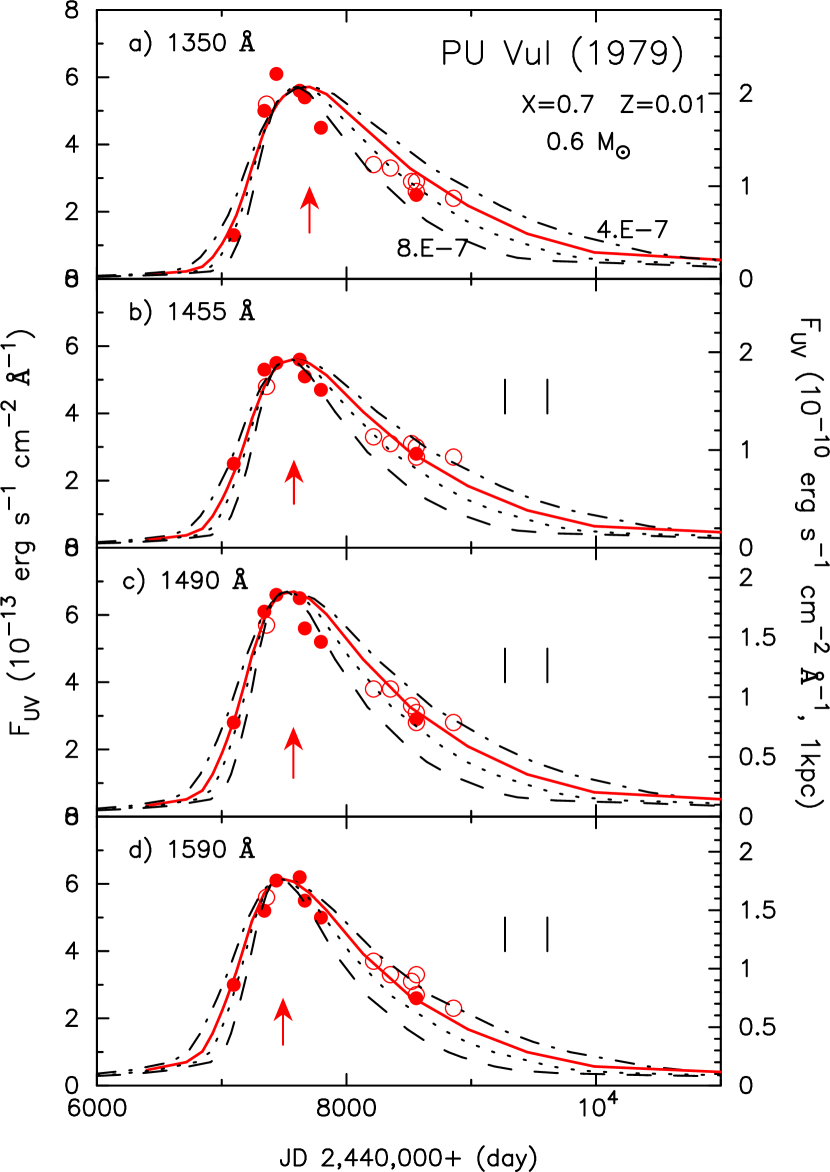
Figure 1.— UV light curves for four narrow bands at, a) 1350 Å, b) 1455 Å, c) 1490 Å, and d) 1590 Å. Theoretical light curves are also shown for an assumed distance of 1 kpc (with right-side axis) and no absorption; They are 0.6 $M_{\odot}$ WDs with the chemical composition of the envelope $X=0.7$ and $Z=0.01$ with four different optically-thin wind mass-loss rates; Dash-dotted curves: $4\times 10^{-7}M_{\odot}$yr^-1. Solid curves: $5\times 10^{-7}M_{\odot}$yr^-1 (Model 1). Dotted curves: $6\times 10^{-7}M_{\odot}$yr^-1. Dashed curves: $8\times 10^{-7}M_{\odot}$yr^-1. Short vertical lines in panels b), c), and d) show the period of the second eclipse at the optical $V$ band between JD 2,449,270 and 2,449,610. Among the observational data, the open circles denote the ones with low accuracy because they were observed with a short exposure time ($<1000$ s) or it is obtained from very noisy spectra. The red arrows indicate the epoch of the UV maximum in each wavelength band.

2.2. Continuum UV Light Curve

In classical novae, a narrow spectral region around 1455 Å  is known to be emission-line free and can be a representative of continuum flux (Cassatella et al., 2002). This continuum band has been used to determine distances to several classical novae (Hachisu & Kato, 2006; Hachisu et al., 2008; Kato et al., 2009), and also used in analysis of PU Vul (Kato et al., 2011). As PU Vul shows much weaker emission lines in its spectra than classical novae, we can use three other wavelength bands around 1350, 1490 and 1590 Å  of a 20  Å  width, in addition to the UV 1455  Å  band. Figure 1 depicts light curves of these four narrow bands, extracted from the IUE data archive.

During the outburst, the photospheric temperature gradually rises and the photospheric radius shrinks while the bolometric luminosity is almost constant. Thus, a UV light curve has the peak at a certain temperature. Figure 1 also shows theoretical UV light curves that represent continuum emission in each wavelength. These four light curves show basically a similar behavior, because each wavelength is close. In a shorter wavelength band, the UV flux reaches maximum slightly later than in the other longer bands as indicated by upward arrows.

The flux at the observed peak is obtained to be $F_{1350}=5.7\times 10^{-13}$, $F_{1455}=5.6\times 10^{-13}$, $F_{1490}=6.7\times 10^{-13}$, and $F_{1590}=6.1\times 10^{-13}$ erg s^-1cm^-2Å^-1, respectively. If the emission can be approximated by blackbody, unabsorbed peak fluxes should be larger in a shorter wavelength band, while the absorbed fluxes are in the inverse order. Comparing these peak fluxes, we see that the 1455 Å  band flux is too small, because the peak flux is more absorbed by cool winds from the M giant companion than in the other three bands of 1350, 1490 and 1590  Å  (Shore & Aufdenberg, 1993). The excess of $F_{1490}$ may be explained by contamination of emission lines. Considering these effects, we use the 1590  Å  band in the following discussion.

Figure 1 also shows model light curves of the 0.6 $M_{\odot}$ WD with the chemical composition of $X=0.7,~{}Y=0.29$, and $Z=0.01$. Each band light curve is made from blackbody emission of our evolution model. Here, we assume four optically-thin wind mass-loss rates of 4–8 $\times 10^{-7}~{}M_{\odot}$ yr^-1. For a higher mass-loss rate, the evolution is faster and the UV light curve shape is narrower. All these light curves more or less agree with the observational UV light curve in each wavelength band, and we chose the $5\times 10^{-7}~{}M_{\odot}$ yr^-1 as having the best agreement with these data points.

For a given chemical composition Kato et al. (2011) obtained a range of the WD mass that reasonably well reproduces the UV light curve for reasonable rates of the optically-thin mass-loss. The lowest WD mass is obtained for a very large wind mass-loss rate of $1\times 10^{-6}M_{\odot}$ yr^-1, while the highest WD mass is for no wind mass-loss. For example, if we fix the chemical composition to be $X=0.7$ and $Z=0.01$, a plausible WD mass is between 0.52 and 0.72 $M_{\odot}$, corresponding to the wind mass-loss rate of $1\times 10^{-6}M_{\odot}$ yr^-1 and no mass-loss, respectively. These ranges of the WD mass are summarized in Table 2 for four specified chemical compositions. This table also shows a range of the bolometric luminosities at the optical flat peak. The larger the bolometric luminosity, the more massive the WD. Combining these theoretical bolometric luminosities with the observed magnitudes, we can derive a range of the distance moduli, $(m-M)_{V}$, which are shown in the last column of Table 2.

Table 2Range of Distance Moduli

Composition		WD Mass	$L_{\rm bol}$	$V_{\rm peak}-M_{\rm V}$
$(X,Y,Z)$		($M_{\odot}$)	($10^{37}$erg s-1)
(0.7, 0.29,  0.01)	…	0.52 – 0.72	3.4 – 6.1	13.87 – 14.52
(0.7, 0.28,  0.02)	…	0.5 – 0.67	3.0 – 5.0	13.75 – 14.30
(0.5, 0.49,  0.01)	…	0.5 – 0.62	3.0 – 5.7	14.03 – 14.45
(0.5, 0.494, 0.006)	…	0.53 – 0.65	4.5 – 6.5	14.19 – 14.58

3. Extinction and Distance

Before deriving physical parameters of the nova, we must estimate the extinction and distance. The reddening was estimated by various methods, H I Balmer line ratios, He II emission line ratios, interstellar optical/UV absorption features, and comparison between the observed optical/near-IR spectra and some standards (Belyakina et al., 1982b, 1984; Friedjung et al., 1984; Kenyon, 1986; Gochermann, 1991; Vogel & Nussbaumer, 1992; Hoard et al., 1996; Rudy et al., 1999; Luna & Costa, 2005). They are unfortunately scattered in a broad range of $E(B-V)=0.22-0.53$. Thus, we have made our own estimates based on the theoretical light curves (Section 3.1) and comparison between spectral classification and colors (Section 3.2).

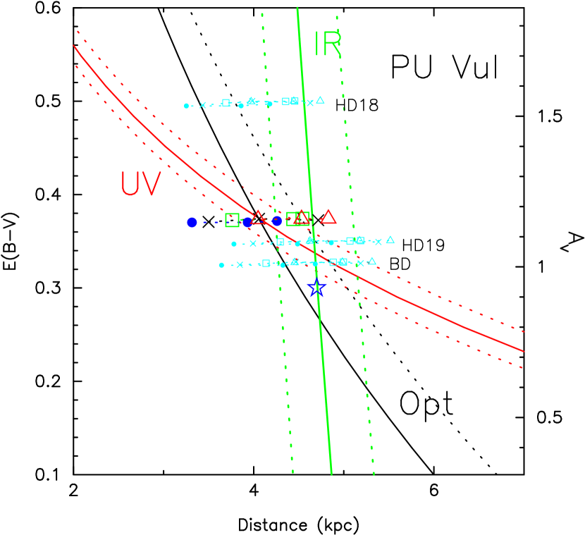
Figure 2.— Distance-reddening relation of PU Vul. The distance-reddening relations obtained from the optical light curve fitting of Model 1; black solid line: $(m-M)_{V}=14.20$, i.e., Equation (2); black dotted line: $(m-M)_{V}=14.44$. The red solid line represents the UV 1590  Å  light curve fitting of Model 1 (Equation (5)). The two red dotted lines beside the line represent possible $\pm 15\%$ errors in absolute UV flux. The distance-reddening relation derived from the K-magnitude fitting (Equation (8)) is depicted by the green solid line with $\pm 0.2$ mag error lines in both sides. The central black cross indicates the intersection of the UV and optical fluxes of Model 1. The crosses in both sides represent the intersections for $M_{\rm WD}=0.52$ (left) and 0.72 $M_{\odot}$ (right) WD models with the chemical composition of $X=0.7$ and $Z=0.01$, i.e., the lowest and highest WD masses in Table 2. Other models are depicted by the different symbols: blue filled circles for Model 2, green open squares for Model 3, red triangles for Model 4. The intersections for the same models but for different extinction law are also plotted by blue symbols: ($R_{V},~{}R_{1590}$)=(2.40, 6.29) for HD185418, (2.48, 8.03) for HD197702, and (2.91, 8.84) for BD +35 4258. The same symbol indicates the same chemical composition and the middle point of the three same symbols corresponds to the models in Table 1. The name of each star is indicated beside the corresponding group of points with first few letters. The open star mark represent $d$=4.7 kpc and $E(B-V)=0.3$. See Section 3.1 for more detail.

3.1. Extinction from Model Light Curves

From our light curve fittings, we get relations on the extinction $E(B-V)$ and the distance $d$ to PU Vul. The distance modulus is

$$(m-M)_{V}=A_{V}+5\log~{}(d/1~{}{\rm kpc})+10,$$ (1)

where $A_{V}=R_{V}\times E(B-V)$ and $R_{V}=3.1$. In the optical maximum phase, 1979-1986, except the eclipse, the mean magnitude is obtained to be $V=8.59\pm 0.06$ (see Table 4), whereas the absolute bolometric magnitude is $M_{\rm bol}=-5.44$ from Model 1 (Table 1). Here, we adopt a bolometric correction of BC($V$)=0.17 (see Section 4), as a representative value for an extended WD photosphere during the A-F spectral phase. Then, we have

$$14.20=3.1\times E(B-V)+5\log~{}(d/1~{}{\rm kpc})+10.$$ (2)

This equation gives a relation between $E(B-V)$ and $d$ for a specified model, Model 1, which is depicted in Figure 2. There is another possible way of fitting. In 1979, PU Vul showed a spectral type of F0 I without emission lines, and its magnitude was about $V=8.87$ (see Figure 8). If we take a bolometric correction typical for F0 I/II, BC($V$)=0.13 (Straizys & Kuriliene, 1981), we have a larger distance modulus $(m-M)_{V}=14.44$ for the same Model 1. This case is also plotted in Figure 2.

We have another distance-reddening relation from the UV 1590  Å light curve fitting, i.e.,

$$-2.5~{}\log F_{1590}({\rm obs}) = -2.5~{}\log F_{1590}({\rm model})$$ (4)

$$+A_{\lambda}+5~{}\log~{}(d/{\rm 1~{}kpc}).$$

Here $A_{\lambda}=R_{1590}~{}E(B-V)$ and we adopt $R_{1590}$=8.3 (Fitzpatrick & Massa, 2007). Seaton (1979)’s formula gives a similar value of $7.9$. Figure 1(d) shows $F_{1590}({\rm obs})=6.1\times 10^{-13}$ erg s^-1 cm ${}^{-2}~{}$ Å^-1 at the UV 1590  Å  peak, whereas $F_{1590}({\rm model})=1.77\times 10^{-10}$ erg s^-1 cm ${}^{-2}~{}$Å^-1 with an assumed distance of $d=1$ kpc. Substituting these values into equation (4), we get a relation

$$6.15=8.3\times E(B-V)+5\log~{}(d/1~{}{\rm kpc})$$ (5)

for Model 1. Figure 2 also shows Equation (5) with two additional lines in the both sides which represent a possible $15\%$ error in the light curve fitting. This error is a summation of the accuracy of the absolute flux calibration of IUE ($\sim 5\%$) and possible contamination of emission/absorption line contribution in the region of 1590  Å, which we assumed to be 10 %.

Combined these two fittings, i.e., Equations (2) and (5), we obtain $E(B-V)=0.37$ and $d=4.1$ kpc, which are plotted by a black X-mark (the middle one among the three Xs). If we assume a different WD mass, we get a different relation between $E(B-V)$ and $d$, because $M_{V}$ is different for a different WD mass model. The two X-marks in the left/right sides in Figure 2 indicate the intersection of the two extreme cases of $M_{\rm WD}=0.52$ and 0.72 $M_{\odot}$, corresponding to the lowest and highest WD masses (see Table 2).

For different sets of chemical composition, we also get different intersections which are shown by different symbols in Figure 2. From these points we see that $E(B-V)=0.37$ is almost independent of the WD mass or chemical composition. This is because we use the same response (passband) functions to derive $M_{V}$ and $\log F_{1590}({\rm model})$ from blackbody spectrum of each model, and therefore, the ratios of the two values are common in all the models. As a result, these two equations yield a common value of $E(B-V)$ independent of the model. On the other hand, the distance depends on the WD mass and chemical composition ($X$), because a more massive WD/smaller $X$ has a larger photospheric luminosity, which results in a larger distance. In this way, we could not determine the distance only from the light curve fittings. We can constrain the distance corresponding to a permitted range of the WD mass as listed in Table 1.

It should be noted that Galactic interstellar absorption has very large uncertainty around the average value we adopted (see e.g. Fitzpatrick & Massa, 2007). Unfortunately, the extinction curve are not known in PU Vul, nor in the stars close to its same sight line. The closest stars are relatively far away; towards HD 185418 and HD 197702 , both $\sim 11\deg$ away from PU Vul, and towards BD +35 4258, $\sim 15\deg$ away. The values of ($R_{V}$ and $R_{1590}$) are (2.40, 6.29) for HD 185418, (2.48, 8.03) for HD 197702, and (2.91, 8.84) for BD +35 4258. Using these values, we obtain the intersection from Equations (1) and (4), which are also shown in Figure 2. These extinction estimates strongly depend on the adopted extinction curve.

Thus, we could not accurately determine the distance and $E(B-V)$ from the light curve fittings of UV/optical bands.

Table 3Color excess in optical

Date	Sp. Type	$<V>$	$<B-V>$	$(B-V)_{0}$	$E(B-V)$	$<U-B>$	$(U-B)_{0}$	$E(U-B)$
Apr 1979	A7 II	8.84	$0.39\pm 0.01$	0.12	0.27	$0.24\pm 0.01$	0.02	0.25
May 1979	F0 I	8.93	$0.42\pm 0.01$	0.19	0.23	$0.29\pm 0.01$	0.16	0.13
May 1979	F0 I	8.98	$0.51\pm 0.02$	0.19	0.32	$0.43\pm 0.03$	0.16	0.27
Jul 1979	F0 I	8.84	$0.44\pm 0.01$	0.19	0.25	$0.34\pm 0.01$	0.16	0.18
Sep 1979	F5 I	8.78	$0.57\pm 0.01$	0.40	0.17	$0.37\pm 0.02$	0.32	0.05
Dec 1979	F3 I	8.78	$0.69\pm 0.01$	0.31	0.38	0.50	0.27	0.23
Aug 1981	F5 I	8.55	$0.75\pm 0.01$	0.40	0.35	$0.47\pm 0.01$	0.32	0.15
Aug 1981	F5 I	8.64	$0.71\pm 0.01$	0.40	0.31	$0.55\pm 0.01$	0.32	0.23
Jun 1982	F5 I	8.50	$0.78\pm 0.01$	0.40	0.38	$0.44\pm 0.02$	0.32	0.12
Sep 1982	F5–8 I	8.67	$0.74\pm 0.01$	0.49	0.25	$0.42\pm 0.02$	0.36	0.06
Nov 1982	F3–4 I	8.40	$0.57\pm 0.01$	0.33	0.24	$0.19\pm 0.01$	0.28	-0.09
Dec 1982	F0 I	8.43	$0.58\pm 0.01$	0.19	0.39	$0.23\pm 0.03$	0.16	0.07
Jul 1983	F0 I	8.39	$0.61\pm 0.01$	0.19	0.42	$0.27\pm 0.01$	0.16	0.11

3.2. Optical Color Excess

A direct estimate of the color excess $E(B-V)$ can be derived from the comparison of observed $B-V$ colors and spectral types of the hot component during 1979-1983, i.e., at the optical maximum when strong emission lines were still absent. In particular, we have calculated one-month averaged $B-V$ and $U-B$ colors from the published photometry (Belyakina et al., 1982a, 1985, 1990; Kolotilov, 1983; Margrave, 1979; Mahra et al., 1979; Whitney, 1979; Bruch, 1980; Chochol et al., 1981; Purgathofer & Schnell, 1982) for several epochs when the spectral classification of PU Vul was made (Kolotilov, 1983; Belyakina et al., 1984; Mürset & Nussbaumer, 1994, and references therein). Table 3 shows the one-month averaged $B-V$ and $U-B$ colors and spectral classification corresponding to each epoch. Assuming that the nova envelope of PU Vul had a typical spectral type, we can estimate the extinction with the comparison to the intrinsic color index corresponding to its spectral type (Straizys, 1992). The $B-V$ and $U-B$ colors of PU Vul are in good agreement with those of bright supergiants for 1979–81, and the average ratio of $E(U-B)/E(B-V)=0.66^{+0.12}_{-0.14}$ estimated for this period agrees with the predicted value of $\sim 0.63-0.69$ (Ciardelli et al., 1989). Since 1982 there is some contamination by the nebular continuum emission, especially in the $U-B$ color. We thus obtain $E(B-V)=0.30\pm 0.02$ for the whole 1979-1983 period, and $E(B-V)=0.29\pm 0.02$ for 1979-81.

This value is in good agreement with the color excesses estimated from various emission line ratios. We estimate $E(B-V)\sim 0.2$–0.3, from our measurements of the He II 1640 emission line fluxes from IUE spectra obtained in October 1991 and August 1992 combined with the optical He II 4686 line fluxes for the same epochs (Andrillat & Houziaux, 1995), assuming electron temperature between 10 000–20 000 K. Similarly, Rudy et al. (1999) derived $E(B-V)=0.22\pm 0.10$ from the O I line ratios whereas Luna & Costa (2005) reported $E(B-V)=0.29$ resulting from the Balmer H I line ratios.

Our extinction estimates agree with estimates for the total Galactic extinction towards PU Vul. We estimated $E(B-V)=0.35$ from the Galactic extinction distribution based on COBE and IRAS maps combined with the Leiden-Dwingeloo maps of H I emissions (Schlegel et al., 1998). Also $E(B-V)\sim 0.2$ is obtained from the dust map based on analysis of 2MASS photometry (Marshall et al., 2006).

3.3. Distance Estimates from Pulsating RG

An independent way of distance estimate comes from the pulsating RG companion of PU Vul. There is a well-known relation between the pulsation period and its luminosity for Mira variables, applicable also to semi-regular variables pulsating in the fundamental mode,

$$M_{K}=-3.51\times(\log P({\rm day})-2.38)-7.25,$$ (6)

with an error of $\sim$ 0.2 mag (Whitelock et al., 2008). For the 218 day pulsation, we get the absolute $K$ magnitude of $M_{K}=-7.10\pm 0.2$. During the 1980 eclipse the average $K$ mag changes from 6.26 mag to 6.51 mag (Belyakina et al., 1985) and its average value is $<K>=6.37\pm 0.04$ mag.

On the other hand, the difference between the absolute and apparent K-magnitudes is written as

$$K-M_{K}=0.353\times E(B-V)+5\log~{}(d/1~{}{\rm kpc})+10,$$ (7)

here we adopt the reddening law of $A_{\rm K}=0.353\times E(B-V)$ (Ciardelli et al., 1989). Therefore, we get

$$13.47=0.353\times E(B-V)+5\log~{}(d/1~{}{\rm kpc})+10.$$ (8)

This relation is plotted in Figure 2. For a particular value of $E(B-V)=0.3$, we get $d=4.7$ kpc. Figure 2 shows that the intersections of the three solid lines, i.e., UV, optical, and IR, are relatively close, and $E(B-V)=0.3$ from optical color excess is also close to these points. This indicates that our various methods are consistent with each other. Considering ambiguity of each method, we use $E(B-V)=0.3$ and $d=4.7$ kpc as a reasonable estimate.

Table 4Temperature and Radius of Hot Component

Date	JD	Spectral	Ion	$V$	$T_{\rm h}$	$M_{\rm bol}$	$L_{\rm h}$	$R_{\rm h}$	Method
	2,400,000+	type			(K)		($L_{\odot}$)	$(R_{\odot}$)
04/1979	43980	A7 II		8.84	7900	-5.36	11070	56	[1]
05/1979	43991	F0 I		8.93	7400	-5.23	9820	60	[1]
07/1979	44070	F0 I		8.84	7400	-5.32	10670	63	[1]
12/1979	44222	F3 I		8.78	6900	-5.41	11590	75	[1]
08/1981	44834	F5 I		8.55	6500	-5.66	14590	95	[1]
09/1981	44873	F5 I		8.50	6500	-5.65	14510	95	[2]
06/1982	45147	F5 I		8.50	6500	-5.71	15280	97	[1]
09/1982	45229	F5-8 I		8.67	6300	-5.57	13430	97	[1]
11/1982	45290	F3-4 I		8.40	6800	-5.79	16440	92	[1]
12/1982	45320	F0 I		8.43	7400	-5.73	15560	76	[1]
07/1983	45533	F0 I		8.39	7400	-5.77	16140	77	[1]
10/1984	45989	A3 I		8.55	8900	-5.77	16140	53	[1]
06/1985	46232	A3 I		8.52	8900	-5.80	16600	54	[1]
09/1986	46690	A2 I		8.72	9200	-5.67	14720	48	[1]
01/1988	47176	–	S+	–	10000	–	–	–	–
06/1988	47328	–	N+	–	15000	–	–	–	–
10/1988	47438	–	N+2	–	35000	-5.43	11800	3.0	[3]
10/1988	47438	–	N+2	–	29000	-5.49	10704	4.4	[3a]
05/1989	47666	–	C+3,N+3	–	40000	-5.47	12230	2.3	[3]
05/1989	47666	–	C+3,N+3	–	48000	-5.47	15440	1.8	[3a]
05-09/1989	47730	–	C+3,N+3	–	48000	-5.70	15140	1.8	[4]
04/1990	47795	–	O+3	–	55000	-5.81	16750	1.4	[4]
07/1990	48088	–	Ne+2	–	41000	-5.64	14320	2.4	[4]
11/1990	48217	–	He+2	–	65000	-5.65	14500	0.95	[5], SWP40155
04/1991	48352	–	He+2	–	65000	-5.64	14350	0.94	[5], SWP41299
09/1991	48522	–	He+2	–	67000	-5.59	13710	0.87	[5], SWP42536
10/1991	48559	–	He+2	–	70000	-5.55	13230	0.78	[5], SWP42937/8
08/1992	48858	–	He+2	–	77000	-5.67	14660	0.68	[5], SWP45415
06/1995	49886	–	Ne+4	–	97000	-5.58	13540	0.41	[6]
06/1995	49886	–	Ne+4	–	97000	-5.68	14860	0.43	[4]
06/1996	50237	–	He+2	–	90000	-5.31	10570	0.42	[5], SWP57322/3
06/1996	50237	–	–	–	90000	-5.42	11700	0.36	[4]
09/1996	50342	–	He+2	–	83000	-5.05	8300	0.44	[5], SWP58251/2
09/2001	52154	–	Fe+6	–	100000	-4.68	5940	0.26	[6]
09/2001	52154	–	Fe+6	–	100000	-5.42	11700	0.36	[4]
26/3/2003	52818	–	Fe+6	–	165000	-4.97	7730	0.11	[4]
9/4/2004	53105	–	Fe+6	–	$>99000$	–	–	–	–
04/2004	53110	–	–	–	150000	-4.97	7720	0.13	[4]
07/2006	53930	–	O+5	–	$>114000$	–	–	–	–
07/2006	53930	–	O+5	–	150000	-4.70	6030	0.11	[4]
06/2011	55740	–	–	–	150000	-5.02	8090	0.13	[4]

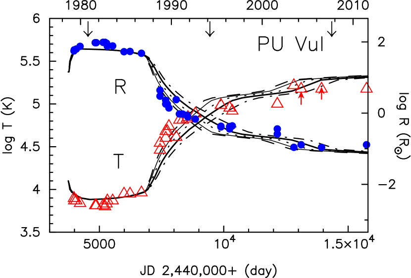
Figure 3.— Development of the temperature (open triangles and the left ordinates) and radius (filled circles and the right ordinates) of the hot component (WD) of PU Vul, taken from Table 4. Two red upward arrows indicate lower limits of temperature. Model lines denote the photospheric temperatures and radii of the 0.6 $M_{\odot}$ WD with $X=0.7$ and $Z=0.01$ for five different wind mass-loss rates. Dash-dotted lines: $4\times 10^{-7}~{}M_{\odot}~{}$yr^-1. Thick solid lines: $5\times 10^{-7}~{}M_{\odot}~{}$yr^-1 (Model 1). Dotted lines: $6\times 10^{-7}~{}M_{\odot}~{}$yr^-1. Thin solid lines: $7\times 10^{-7}~{}M_{\odot}~{}$yr^-1. Dashed lines: $8\times 10^{-7}~{}M_{\odot}~{}$yr^-1. Three black downward arrows indicate the central times of the 1980, 1994, and 2007 eclipses.

4. Evolution of Temperature and Radius

We have deduced the temperature and total luminosity of the hot component (WD) of PU Vul using IUE spectra as well as published photometry and other useful information. The radius is calculated from the temperature and luminosity using the Stefan-Boltzmann law. Here we assume $E(B-V)=0.30$ and $d=4.7$ kpc. We use the extinction law of Fitzpatrick & Massa (2007) for the narrow band continuum and emission lines, and Ciardelli et al. (1989) for the broad band optical and near infrared photometry, respectively. The resulting values are listed in Table 4. For several epochs we have been able to calculate them using more than one method, and the differences in the results give an idea about the uncertainties of these methods.

The third column of Table 4 shows the spectral classification adopted from Kolotilov (1983), Belyakina et al. (1984), and Mürset & Nussbaumer (1994, Table 3), and the fifth column shows the average of observed $V$ magnitudes (Kolotilov, 1983; Belyakina et al., 1982a, 1985, 1990) of PU Vul during the optical maximum, 1979–1986. The outbursting component of PU Vul showed spectra similar to that of an early F-type supergiant, gradually evolving towards an A supergiant. Since there is no strong nebular contribution during this phase, we have assumed that the spectral type is an appropriate indicator for the effective temperature and bolometric correction, and that the observed $V$ magnitude (Kolotilov, 1983; Belyakina et al., 1982a, 1985, 1990) represents that of the hot component. We have adopted the temperatures and bolometric corrections for A-F supergiants from Straizys & Kuriliene (1981), and adopt $M_{\odot}$(bol)=4.75 for the absolute bolometric luminosity of the Sun.

The hot component luminosity in September 1981 (JD 2 444 873) have been estimated directly by integrating the spectral energy distribution (SED) from ultraviolet to infrared. To get the SED we have combined the very long exposure IUE spectra (SWP 15110, LWR 11627 and LWR 11628) from 27 September 1981 with Belyakina et al. (1985) spectrophotometry performed on 25 September 1981 and $JHK$ photometry obtained on 22 September 1981. The SED has been corrected for the reddening. The resultant bolometric magnitude is $m_{\rm bol,0}=7.71$, which derives the absolute bolometric magnitude $M_{\rm bol}=-5.65$ with the distance $d=4.7$ kpc. This value, $-5.65$, shows an excellent agreement with the average value, $-5.66$ in August 1981, derived from the observed $V$ mag and spectral type (see Table 4).

We have also used this SED to estimate the bolometric correction corresponding to this particular date, in September 1981. We obtain $V_{0}=7.57$ from the SED. Thus, the bolometric correction is calculated as BC$(V)=m_{\rm bol,0}-V_{0}$ = 0.14. On the other hand, Belyakina et al. (1985) obtained $V=8.45$ on JD 2 444 873, which is corrected to be $V_{0}=7.52$ with an extinction of $3.1\times E(B-V)$=0.93. Combining this with $m_{\rm bol,0}=7.71$, we get BC$(V)=0.19$. These BC$(V)$ values are somewhat larger than BC$(V)=0.08$ corresponding to F5 I spectral type estimated at this epoch. The difference may reflect the lower density in the nova envelope than that in the brightest F-type supergiants. In the present work, we use BC$(V)=0.17$, the mean value of 0.14 and 0.19.

For the nebular phase, whenever possible, the temperature of the hot component (WD), $T_{\rm h}$, has been estimated from the equivalent width of the He II 1640 emission line measured from IUE spectra (identified in the last column of Table 4). Although the high resolution HST/GHRS spectrum taken in October 1994 (the 1993/4 eclipse egress) suggest $\sim 20\%$ of O I]1641 line contribution to the He II fluxes derived from lower resolution spectra, the O I]1641 line is not visible in the well exposed high resolution spectra SWP45417 and SWP57730 taken before and after the eclipse, respectively. Therefore, we assume a negligible contribution of O I] to our measurements of the He II 1640 line. The luminosity of the hot component, $L_{\rm h}$, has been calculated from the He II 1640 flux, assuming blackbody ($T_{\rm h}$) and that the He II lines are produced by photoionization followed by recombination (case B). $L_{\rm h}$ has been also estimated from the IUE flux at 1350  Å, assuming that it is emitted by blackbody ($T_{\rm h}$). At most epochs in Table 4 these two values agree with each other, and a mean value is adopted for the final $L_{\rm h}$.

At several epochs, $T_{\rm h}$ has been derived from the highest ionization potential (IP) observed in the IUE spectra (JD 2 447 438–795) and published optical spectra (Munari & Zwitter, 2002; Yoo, 2007; Tatarnikova & Tatarnikov, 2011). We used the relation $T_{\rm h}$/1000 $\sim$ IP (eV) found by Mürset & Nussbaumer (1994). For two epochs of JD 2 452 154 and 2 452 818, $T_{\rm h}$ is derived from the ratios of H$\beta$, He II 4686 and He I 5876 emission line fluxes published by Tatarnikova & Tatarnikov (2011) and Luna & Costa (2005), respectively.

At two epochs of 1988 and 1989, the hot component parameters have been derived by fitting a blackbody to the short wavelength ($\lambda\lesssim 1590$  Å) part of the spectrum obtained by combining SWP34405, SWP34406, and SWP34407 for JD 2 447 438, and SWP36301, SWP36302 and SWP36304 for JD 2 447 666.

After 1996, in the absence of IUE spectra, $L_{\rm h}$ has been derived from the $UB$ mag observed by Belyakina et al. (2000) and by Shugarov et al. (2011) with the method proposed by Mürset & Nussbaumer (1994). This method assumes that after subtraction of the contribution from the RG, the optical magnitudes contain a direct contribution from the hot star and an indirect contribution from the nebulae. Thus, an accurate estimate of the RG contribution is especially important. The RG companion is classified to be a spectral type of M6 (Section 5.1), so its contribution to $UB$ magnitudes can be neglected. In fact, the $B-V$ and $U-B$ colors (Shugarov et al., 2011) suggest that the continuum is still dominated by the nebular emission, in agreement with the optical spectra showing only faint flat continuum and strong emission lines (e.g. Yoo, 2007). As described later (Sections 5 and 6 and Figure 8), the summation of the WD and nebular contributions dominates the $V$ light curve, although it shows a clear $\sim 0.5$ mag pulsation owing to the RG. Therefore, we can safely use the method of Mürset & Nussbaumer (1994). Mürset & Nussbaumer (1994) also provided the bolometric corrections to $UBV$ mag of hot component for a wide range of hot component temperature, $T_{\rm h}$. These bolometric corrections were derived by model calculations with hot component temperature and nebular density as free parameters. Although the RG in PU Vul is similar to a Mira component of D-type symbiotic systems, we have decided to use the bolometric corrections for S-types because the $U-B$ color of PU Vul during the nebular phase is similar to that predicted by the Mürset & Nussbaumer (1994) model for S-types, and the electron density derived for the nebular phase is similar to the values characterizing the other S-type systems (Luna & Costa, 2005).

At JD 2 449 886 and JD 2 452 154, the luminosity of the hot component, $L_{\rm h}$ has been calculated from the published He II 4686 fluxes (Andrillat & Houziaux, 1995; Tatarnikova & Tatarnikov, 2011), assuming a blackbody spectrum with $T_{\rm h}$ and that the He II lines are produced by photoionization followed by recombination (case B).

Our estimated temperature and radius are plotted in Figure 3. This figure also shows theoretical models for the 0.6 $M_{\odot}$ WD with the composition of $X=0.7$ and $Z=0.01$, i.e., the same models as in Figure 1. The higher the mass-loss rate, the faster the evolution. All of these models show more or less good agreement with our observational estimates. It should be noticed that the theoretical values are those of a blackbody photosphere. Even though, they show good agreement with the IUE flux (Figure 1) and also with the estimates obtained with quite different methods (Table 4).

Figure 4 shows the HR diagram of the hot component. This figure shows theoretical tracks of the 0.5, 0.6 and 0.7 $M_{\odot}$ WDs for various chemical compositions. The observational estimates are also in good agreement with our 0.6 $M_{\odot}$ models.

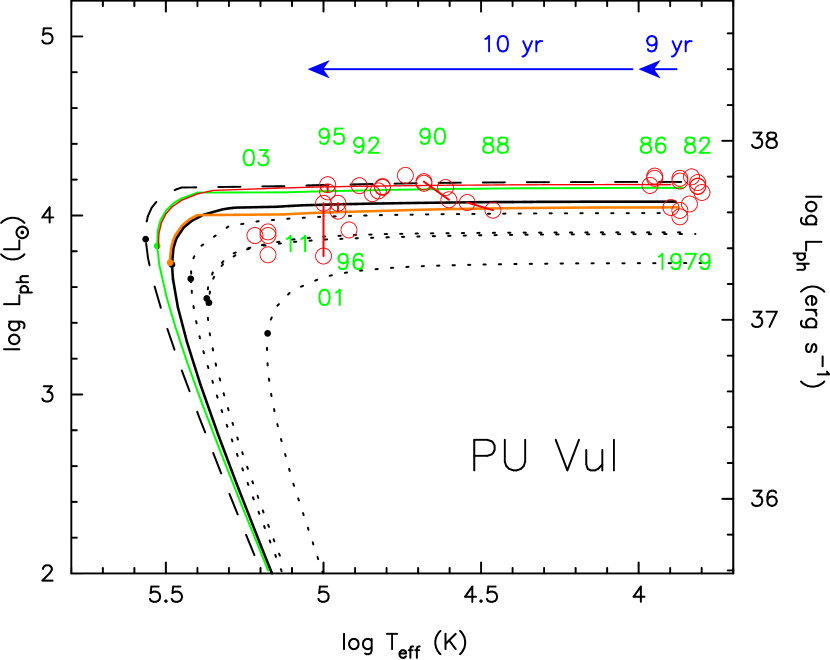
Figure 4.— Evolution of the hot component of PU Vul in the HR diagram. Red open circles are our observational estimates, taken from in Table 4. Pairs connected by a line segment indicate the estimates obtained for the same day data but with different methods. Observational years (two digits except 1979) are attached beside the point. Various types of lines denote loci of theoretical models. Solid lines indicate, from upper to lower, Model 4 (red), Model 3 (green), Model 1 (black), and Model 2 (brown). A dashed line denotes a 0.7 $M_{\odot}$ WD with $X=0.7$ and $Z=0.01$. Four dotted lines denote 0.5 $M_{\odot}$ WD models with different radius and chemical compositions. From upper to lower, a cold WD (the Chandrasekhar radius) with $X=0.5$ and $Z=0.02$, a cold WD with $X=0.7$ and $Z=0.01$ (upper) which is almost overlapped with a cold WD with $X=0.7$ and $Z=0.02$ (lower). The lowest line denotes a hot WD with $X=0.7$ and $Z=0.02$. Dots represent the epoch when nuclear burning extinguishes. Arrows indicate evolution timescales of Model 1; from the beginning to $\log T_{\rm ph}$ (K)=4.0, and from $\log T_{\rm ph}$ (K)=4.0 to 5.05, i.e., 8.7 yr and 9.6 yr, respectively.

5. Light Curve Models of Eclipses

Now we present light curve models of the first (1980) and second (1994) eclipses. Here we assume spherical shapes of the both components, that the inclination angle of the orbit is $i=90^{\circ}$, that the RG moves in front of the hot component (WD) with a constant velocity $V_{\rm orb}$, and that the RG is radially pulsating with a period of 218 days and its flux changes in a sinusoidal shape around the equilibrium magnitude. We also assume that the radius of the RG also varies in a fashion of long-period Mira variables (Thompson et al, 2002; Woodruff et al., 2004, 2008), and that the radius varies sinusoidally with a phase shift of 0.5 to the flux variation, i.e., the radius reaches the minimum at the maximum brightness as reported by Shugarov et al. (2011). No accretion disk is assumed, because there is no observational indication.

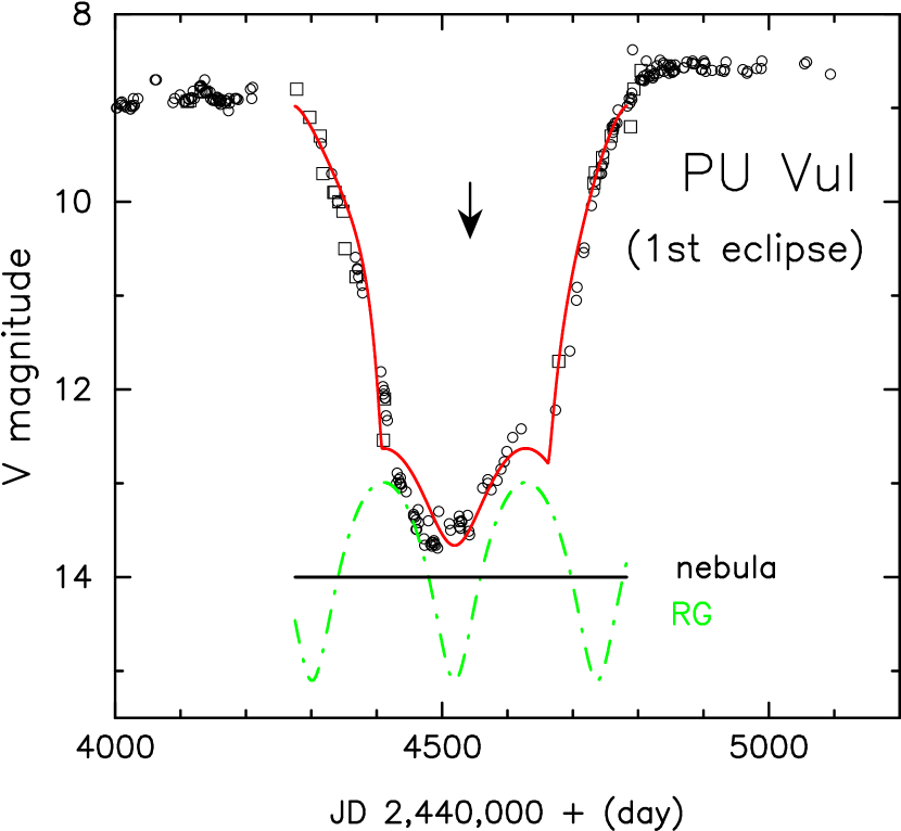
Figure 5.— A close up view of the first eclipse. Our model light curve is indicated by the red solid line, which is a summation of the eclipsed WD photosphere, a constant nebular emission of $V=14.0$, and the RG photosphere with a sinusoidal oscillation around $V=13.6$ (green dash-dotted line). The mideclipse on JD 2,444,532 is indicated by a downward arrow. See text for more details.

Table 5Eclipse Light Curve Model

Subject		1st eclipse	2nd eclipse	Units
mideclipse	…	4,532	9,447	JD 2,440,000+
total duration (D)	…	508	345	day
totality (d)	…	254	343	day
mean RG magnitude	…	13.6	13.6	mag
amplitude of RG luminosity	…	75 %	65 %
total amplitude of RG in mag	…	2.1	1.7	mag
amplitude of RG radius	…	7 %	3 %
$R_{\rm c}/a$	…	0.246	0.22
$R_{\rm h}/a$	…	0.070	0.0007
nebular emission	…	14.0	see Fig. 6	mag

5.1. The First (1980) Eclipse

We suppose that the 1980 eclipse is total, in which the bloated WD is completely occulted by the pulsating RG companion. The bottom magnitude of $V\sim 13$ during the eclipse seems to be a bit higher than that of a late type M-giant, which suggests the presence of a weak emission source which was not occulted. Before going to our model construction, we need to examine the magnitude of the M-giant companion.

The spectral classification of the RG companion is estimated to be M3–M7, but better estimates are obtained in longer wavelength bands rather than in the optical because of contamination by nebular emission. Mürset & Schmid (1999) obtained M6–7, using the bands in near IR, i.e. $\lambda\gtrsim 8000$  Å. Belyakina et al. (1985) derived a similar type, M6.5, during the 1980 eclipse. This value is uncorrected for the faint nebula ($V\sim 14$), so there may be some fluctuations by $\pm 1$ in the spectral type. Therefore, we regard M6 as a reasonable average spectral type of the M-giant.

The magnitude of the RG can be estimated from its $K$-band magnitude. Belyakina et al. (1985) obtained $<K>=6.37$ during the eclipse, and its reddening corrected value is $<K>_{0}=6.26$ (see Section 3.3). A similar value is obtained $<K>_{0}=6.17\pm 0.01$ from Belyakina et al. (2000) and Tatarnikova & Tatarnikov (2011) for an average over 1989–2009. As $V-K\sim 7.2$ for an M6 III star, (e.g. Straizys, 1992), we get $<V>_{\rm 0}\sim 13.4$. Assuming $E(B-V)=0.3$, the visual magnitude of the giant becomes $<V>\sim 14.3$. This value is consistent with an averaged pre-outburst magnitude of $V=14.1\pm 0.15$ (Stephenson, 1979) and $B=16.5$ (Liller & Liller, 1979). This magnitude $<V>\sim 14.3$ is much darker than the observed mean magnitude of $V\sim 13$ at the bottom of the eclipse, so we need an additional source of emission possibly originated from optically-thin plasma such as heated RG cool winds.

We have constructed an eclipse light curve model, assuming that the RG mean magnitude, amplitude of the pulsation, and brightness of the additional emission source are free parameters. Figure 5 shows a close-up view of the first eclipse and our light curve model.

A model light curve, that produces a better fit to the observed magnitude data, is shown in Figure 5. We obtain the total duration of the eclipse $D=508$ days, the totality $d=254$ days, and $R_{\rm c}^{*}/a=(D+d)/(2\pi P_{\rm orb})=0.244$, where $a$ is the separation of the two stars, $P_{\rm orb}$ is the orbital period in units of day, and the asterisk denotes the specific radius, because it depends on the timing of pulsations at the ingress/egress. The equilibrium radius of the pulsating RG is $R_{\rm c}=0.247~{}a$. The RG radius is smaller than the equilibrium radius at the second and third contacts, i.e., 0.93 and 0.96 times the equilibrium radius, we obtain $R_{\rm c}/a$ slightly larger than $R_{\rm c}^{*}/a$.

A bottom magnitude is obtained as a combination of the RG equilibrium magnitude and the nebular emission. An equilibrium magnitude of the RG darker than $V=13.8$ does not reproduce the wavy bottom shape, even if we assume a very large amplitude of the luminosity. A combination of the RG equilibrium magnitude of $V=13.6$ – 13.8 and a nebular emission of $V\sim 14.0$ yield a better fitting as shown in Figure 5. Here we assume the RG equilibrium magnitude to be $V=13.6$ and the nebular emission $V=14.0$.

For the oscillation of the RG radius, a good fitting is obtained for amplitudes of the radius $\Delta R_{\rm c}/R_{\rm c}=$ 0.06–0.08. For a larger amplitude $\Delta R_{\rm c}/R_{\rm c}\gtrsim 0.1$, we cannot find a good shape of light curves, because a wavy structure appears during the ingress and egress. Here, we adopt $\Delta R_{\rm c}/R_{\rm c}=0.07$.

Our fitting parameters are summarized in Table 5, showing the mideclipse time, i.e., the time when the RG center comes just in front of the WD, the total duration of eclipse ($D$), totality ($d$), apparent magnitude of the RG at its equilibrium state, amplitude of the RG luminosity in linear scale $\Delta L_{V}/L_{V}$, corresponding to the total amplitude in magnitude (difference between the maximum and minimum magnitudes), amplitude of the RG radius, the ratio of the RG radius to the separation $a$, and the ratio of the WD radius to $a$. Note that the RG magnitude at equilibrium is not the arithmetic mean of the maximum and minimum magnitudes, because we assume a sinusoidal variation in the luminosity (linear scale), not in the magnitude (logarithmic scale).

Garnavich (1996) supposed that this eclipse is partial because of a non-flat bottom. Vogel & Nussbaumer (1992) explained this non-flat bottom shape as a total eclipse, but contaminated by two nebular emissions that cause the flux excess in the early half and later half, respectively. However, the wavy bottom shape in Figure 5 is consistent with the RG pulsation.

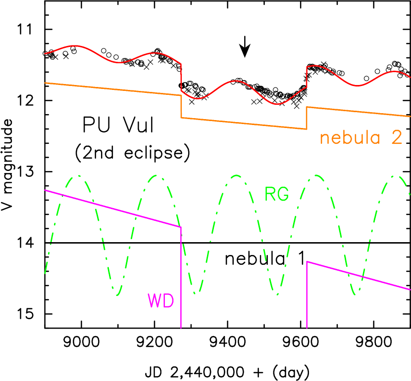
Figure 6.— A close up view of the second eclipse. Observational data are taken from Kolotilov et al. (1995) (crosses) and Yoon & Honeycutt (2000) (open circles). The red solid line indicates our composite light curve which is a summation of the four components, i.e., the pulsating RG (green dash-dotted line), WD (magenta solid line), constant “nebula 1” emission of $V=14.0$ (black solid line), and gradually decreasing “nebula 2” emission which is eclipsed by 25 % (brown solid line). The RG is pulsating around its mean magnitude of $V=13.6$. The mideclipse on JD 2,449,447 is indicated by a downward arrow.

5.2. The Second (1994) Eclipse

PU Vul began to decline in 1987 from the flat maximum and reached $V\sim 11.5$ just before the second eclipse in 1994. The bottom magnitude of the second eclipse is $V\sim 11.8$ (see Figure 6), 1.8 mag brighter than that of the 1980 eclipse. This eclipse is considered to be total, because the continuum UV radiation, which has a WD origin, was disappeared during the eclipse (Nussbaumer & Vogel, 1996; Tatarnikova & Tatarnikov, 2009). Therefore, the excess flux ($\Delta V\sim 1.8$ mag) is a contribution of hot nebulae.

Nussbaumer & Vogel (1996) analyzed UV spectra of the hot nebulae and found that highly ionized lines disappeared during the eclipse and recovered after that, whereas low-ionized nebular lines were hardly affected. This means that the high excitation lines were emitted from a region close to the WD and the low-ionized nebular lines are emitted from an outer extended region. In other words, the nebulae are also partially occulted.

Thus, there are three sources of emission: the pulsating RG, totally occulted WD, and partially occulted nebulae. For the RG, we assume a similar model as in the first eclipse, i.e., the RG is pulsating around the equilibrium magnitude of $V=13.6$ but maybe with different amplitudes of the luminosity and radius, which are fitting parameters. For the WD emission, we take Model 1, which is shown in Figure 6 (labeled as WD). We assume two sources of nebular emission, one is a constant component (labeled “nebula 1”) assumed in the first eclipse, i.e., $V=14.0$. The other is a decreasing component which is partially occulted during the second eclipse (labeled “nebula 2”). Its luminosity and decline rate are also parameters in order to obtain the best fit.

Figure 6 shows the resultant light curve. The amplitude of the luminosity is determined to be 65 % and that of the radius is 3 %. For the nebula 2 component, we found that a 25 % occultation of the nebula 2 emission yields the best fit. We see that our composite light curve represents the temporal change of the optical data.

These fitting parameters are summarized in Table 5. It is difficult to obtain the WD radius from the light curve fitting because the ingress and egress of the second eclipse is very steep, which indicates the eclipsed object is very small. Therefore, we fixed the WD radius to be $R_{\rm h}/a=0.0007$, which corresponds to $1.0R_{\odot}$ for a circular orbit of a binary consisting of a $1.0M_{\odot}$ RG and a $0.6M_{\odot}$ WD. This assumption has no effects in determining the other parameters.

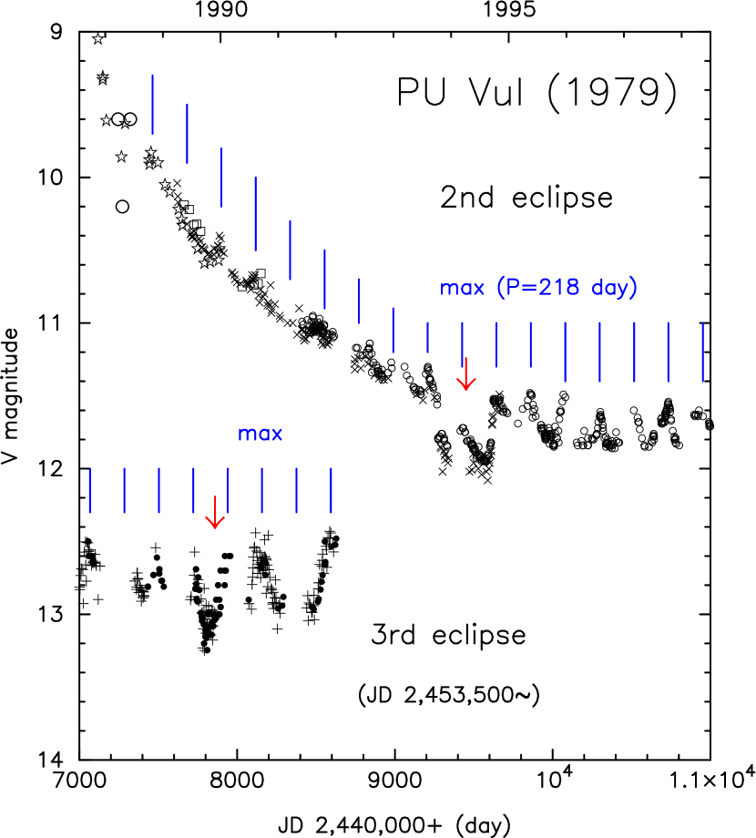
Figure 7.— Light curve of PU Vul for the period JD 2,447,000–2,451,000 (upper part) and JD 2,453,500–2,457,500 (lower part). Observational data are taken from Kolotilov et al. (1995)(crosses), Yoon & Honeycutt (2000)(small open circles), Klein et al. (1994)(squares), Kanamitsu et al. (1991)(open stars), and Iijima (1989)(middle size open circles). For the lower part, observational data are taken from AAVSO (dots) and All Sky Automated Survey (ASAS) (crosses). Downward arrows indicate the central times of the eclipses, JD 2,449,447 and 2,454,362. Short vertical lines indicate epochs of the pulsation maxima of the M giant assuming a period of 218 days.

5.3. M-giant Pulsation and 3rd Eclipse

Figure 7 shows a periodic modulation of the $V$ magnitude, which becomes prominent in the later phase of the outburst where the WD component becomes dark. This modulation is unclear in the flat maximum except the first eclipse (Figures 5), because the hot component is dominant. We regard that this modulation is caused by a pulsation of the RG.

We obtained the pulsation period to be 218 days, assuming that the period is unchanged from the first eclipse until 2010. This 218 day period can reproduce well both the first and second eclipses as shown in Figures 5 and 6. Chochol et al. (1998) obtained a 217 day period and Shugarov et al. (2011) obtained a 217.7 day period. Our value is consistent with these periods.

Figure 7 shows that one of the minima of the RG pulsation accidentally coincides with the time expected for the third eclipse in 2007 indicated by an arrow. This narrow dip is not the third eclipse of the WD, because the duration is too short, and the WD had already become very dark in the optical band (see Figure 8), and an occultation of the WD hardly changes the total brightness of PU Vul. Shugarov et al. (2011) showed that the $U$ magnitude is clearly eclipsed in the third eclipse, but the $V$ magnitude is not. Our interpretation is consistent with theirs.

Table 6Radii of the Cool and Hot Components

RG mass		$a$	$R_{\rm c}$(1st)	$R_{\rm c}$(2nd)	$R_{\rm h}$(1st)
$(M_{\odot}$)		($R_{\odot}$)	($R_{\odot}$)	($R_{\odot}$)	($R_{\odot}$)
3.0	…	1860	459	413	131
2.0	…	1670	411	370	118
1.5	…	1550	383	345	109
1.0	…	1420	350	315	100
0.8	…	1360	335	301	95.6
0.6	…	1290	318	286	90.9
0.4	…	1210	299	269	85.5

5.4. Radii of Cool/Hot Components

In Sections 5.1 and 5.2 we have obtained $R_{\rm c}/a$ and $R_{\rm h}/a$ for the first and second eclipses. Assuming a circular orbit, we calculated the binary separation $a$ from Kepler’s third law, $a^{3}=G(P_{\rm orb}/2\pi)^{2}(M_{\rm WD}+M_{\rm RG})$. The resultant radii of the RG and WD are listed in Table 6 as well as $a$ for various RG masses. Here we assume a 0.6 $M_{\odot}$ WD mass. Estimated RG radii (270 – 460 $R_{\odot}$) seem to be a little bit larger than those of low mass M giant stars, which will be discussed in Section 7 (Discussion).

For the hot component, we obtain a radius of $R_{\rm h}/a=0.07$ for the first eclipse, that corresponds to $R_{\rm h}\sim$ 85–130 $R_{\odot}$ as shown in Table 6. For the second eclipse, we have fixed the WD radius to be $R_{\rm h}/a=0.0007$, because the ingress and egress are too steep to determine the radius. Thus, it is not listed in the table. The steep decline/rise suggest $R_{\rm h}/a<0.001$ which corresponds to $R_{\rm h}<$ 1–2 $R_{\odot}$. We can only say that the radius of the hot component reduced by a factor of 100 or more.

In Section 4 we have already shown that the WD photosphere had shrunk by about two orders of magnitudes between the first and second eclipses, from both the observational estimates and theoretical models (see Figure 3). The above radius estimates from the eclipses are very consistent with these estimates in Figure 3. This is the first time that the shrinkage of a nova WD photosphere has been measured by eclipse analysis.

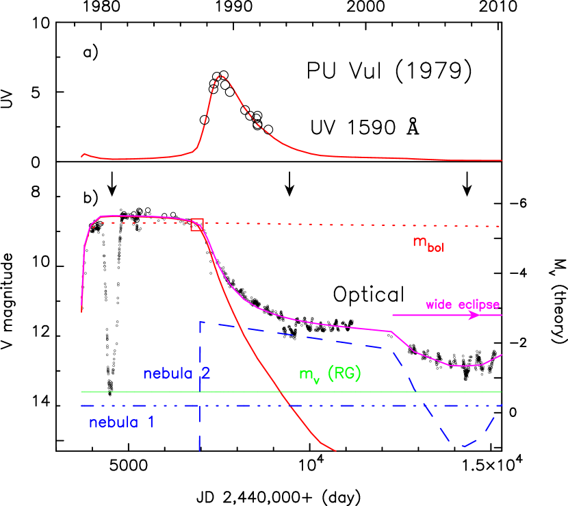
Figure 8.— Optical and UV light curves of PU Vul. (a) UV light curve. Large open circles denote the IUE UV 1590 Å  band (the same as those in Figure 1d). The solid curve denotes the UV light curve of Model 1. The scale is in units of $10^{-13}$ erg s^-1 cm^-2 Å^-1. (b) Optical light curve. Middle size open circles are $V$ magnitudes during the flat phase listed in Table 4. See Kato et al. (2011) for the other observational data. The red solid and dotted lines indicate optical and bolometric light curves of Model 1. The large open square indicates the epoch at $\log T_{\rm ph}$(K)=4.0 when the optically thin wind of $5\times 10^{-7}$ $M_{\odot}$ yr^-1 started in our model. The magenta solid line indicates a composite light curve of the WD (red solid line), RG at the mean luminosity $V=13.6$ (horizontal green solid line), emission of a constant component at $V=14.0$ (“nebular 1”: blue dash-three-dotted line), and a variable component (“nebular 2”: blue dashed line). Downward arrows indicate the mideclipses. We suppose that the “nebula 2” is eclipsed by the RG companion after 2002 (denoted by ’wide eclipse’).

6. Composite Optical Light Curve

Figure 8 shows an observational light curve of PU Vul from the beginning of the outburst until 2010. It also depicts our theoretical composite light curve that consists of three components, the WD, RG, and nebulae. The WD component, in which we use Model 1, well reproduces the observed UV light curve (Figure 8a) as well as the optical light curve until 1989. After 1989, PU Vul entered a nebular phase and emission-lines dominate the spectra (Iijima, 1989; Kanamitsu et al., 1991). Our WD model does not include line-emission formed outside the photosphere, thus the $V$-light curve (red solid line) decays much faster than the observed one. For the RG component, we assume that the equilibrium magnitude is constant, $V=13.6$, throughout the outburst as we did in the first and second eclipses in Section 5. This $V=13.6$ is indicated by the green horizontal solid line in Figure 8b.

For the nebular emission, we assume two components: one is a constant component of $V=14.0$ as depicted by the dash-three-dotted line (nebula 1) in Figure 8b. We assumed this component uneclipsed at all during the first and second eclipses as shown in Figures 5 and 6. We suppose this nebula 1 emission originated from the RG cool wind, partially ionized by the radiation from the hot component. As this emission is faint, it dominated the total magnitude only in the first eclipse, so we have no information on its magnitude whether it changed or not. Therefore, we assumed that this component is constant. Tatarnikova & Tatarnikov (2011) found the Raman scattered O VI 6830 line in the optical spectra taken in mid 2006 and later. This indicates the presence of neutral hydrogen, i.e., the RG cool wind. As the WD is still hot, a part of the RG cool wind may be ionized. So we reasonably suppose this component is still present.

The other nebula is originated from the WD, the shape of which is represented by the blue dashed line (nebula 2). This component started at the epoch when the photospheric temperature of the WD increased to $\log T$ (K)=4.0 (open square in Figure 8). This WD-origin component was first discussed by Nussbaumer et al. (1988), who concluded that the nebular emission is of WD-origin because the relative abundances of C, N, and O are close to those of classical novae but different from symbiotic stars. This component was eclipsed during the second eclipse as in Figure 6.

Recently, Shugarov et al. (2011) reported that all of the $U$, $B$, and $V$ magnitudes are gradually rising after the third eclipse while the mean value of the $I$ magnitude is almost constant. This indicates that the WD-origin nebular component is relatively centrally condensed around the WD and, at the same time, widely spread out over the orbit. Then the width of eclipse by the RG is so wide that a whole period of the orbital phase is partially eclipsed as shown by the blue dashed line in Figure 8. This increase in the brightness ($U$, $B$, and $V$) also suggests that the hydrogen shell-burning on the WD is still on-going.

7. Discussions

7.1. Comparison with Other Works on Eclipses

Garnavich (1996) estimated the relative size of the cool component to be $R_{\rm c}/a=0.28$ for the first eclipse and $0.22$ for the second eclipse, assuming symmetric shapes of the eclipses. Our corresponding values are $R_{\rm c}^{*}/a=0.24$ and 0.22, respectively. The difference in the first eclipse is explained from the difference in the totality. Assuming that the bottom base line at the first eclipse was $V=11.8$ from the second eclipse, Garnavich get a larger totality than ours. Thus, $R_{\rm c}/a$ becomes larger than ours. In the second eclipse our $R_{\rm c}/a$ is essentially the same as Garnavich’s, because the radius oscillation of the RG has little effects due to small amplitude (3 %).

For the hot component, Garnavich (1996) estimated $R_{\rm h}/a=0.1$ for the first eclipse, which is consistent with our value of $R_{\rm h}/a=0.07$, considering difficulty of accurate fitting with the scattered data. For the second eclipse Garnavich’s value $R_{\rm h}/a=0.02$ is much larger than our value of $R_{\rm h}/a=0.0007$. This difference comes mainly from the different data sets. Garnavich used the AAVSO data that show slower decline/increase at the ingress/egress than those in Figure 6. These AAVSO data, however, can be also fitted by a more steep light curve that yields $R_{\rm h}/a<0.01$. Therefore, in the both cases, we can say that the radius of the hot component had decreased at least by a factor of ten between the first and second eclipses.

Garnavich (1996) concluded that the RG radius shrunk by 21 % between the first and second eclipses, i.e., from $R_{\rm c}/a=0.28$ to 0.22. Our values are much smaller, 10 % (from $R_{\rm c}/a=0.246$ to 0.22), but the shrinkage of the radius seems to be real because we cannot find a parameter set for the same RG radius between the two eclipses. We will discuss the shrinkage of the radius in the next subsection.

The orbital period of PU Vul is estimated from the mideclipses of the first and second eclipses to be 4915 days (13.46 yr) (see Table 5). The orbital period was obtained as $4918\pm 8$ days (Kolotilov et al., 1995), $4900\pm 100$ days (Nussbaumer & Vogel, 1996), $4900\pm 9$ (Garnavich, 1996), 4897 days (Shugarov et al., 2011), assuming symmetric shapes of the eclipses. Our analysis first includes a radius oscillation and the resulted non-symmetric shapes of eclipses. However, these effects cause only several days off from the symmetry center because of small amplitudes of the radial oscillations. This is the reason why our new period is close to the previous estimates.

7.2. Comparison with Other Evolution Calculations

Figure 4 shows the evolution timescale of Model 1, 18.3 yr from the beginning of the outburst to $\log T_{\rm ph}$ (K)=5.05. If we do not include the optically-thin wind mass-loss, this becomes 46 yr, and the total duration of the outburst, from the beginning to the extinguish point of nuclear burning, is 130 yr. Using a hydrodynamical code Prialnik & Kovetz (1995) calculated multicycle nova evolution models for various WD masses and accretion rates. For a $0.65~{}M_{\odot}$ WD and a mass accretion rate of $1\times 10^{-7}M_{\odot}$yr^-1, no optically thick wind mass-loss arose. They obtained the total duration of the nova outburst to be $t_{\rm 3bol}$=155–176 yr, depending on the core temperature, where $t_{\rm 3bol}$ is the time during which the bolometric luminosity drops by 3 mag. For lower accretion rates ($\leq 10^{-8}M_{\odot}$yr^-1) strong optically thick winds occur which shorten the total duration. Their total duration is very consistent with our $0.6~{}M_{\odot}$ WD model, considering the different definition of the end point of a shell flash; Our definition is for the hydrogen burning extinguish point (depicted by the dot in Figure 4), whereas Prialnik & Kovetz’ is for $t_{\rm 3bol}$ time which comes later than our extinguish point, thus gives a longer timescale than ours.

Following the referee’s suggestion we discuss the work by Cassisi et al. (1998) and Piersanti et al. (1999, 2000) who calculated shell flashes on low-mass WDs using a spherical symmetric hydrostatic code with the Los Alamos opacity. Cassisi et al.’s (1998) models show that the envelope extends only down to $\log T_{\rm ph}$ (K)=4.5–4.7 for a 0.5 $M_{\odot}$ WD with mass accretion rates of 2 and 4 $\times 10^{-8}M_{\odot}$yr^-1. Also in Piersanti et al. (2000), the temperature decreases down to $\log T_{\rm ph}$ (K) =4.1–4.2 only in a few exceptional cases. Such high-temperature shell flashes may be observed as a UV flash. In other words, these calculations do not represent realistic nova outbursts in which the surface temperature drops to $\log T_{\rm ph}$ (K)$~{}<~{}4.0$ at the optical peak. This suggests that their numerical code has some difficulties in calculating realistic nova outburst models.

It should be pointed out that the above three works are obtained with the Los Alamos opacity, not with the OPAL opacity (Rogers & Iglesias, 1992; Iglesias & Rogers, 1993, 1996), which has been widely used in stellar evolution codes including nova outbursts. We are puzzled by the remark in Cassisi et al. that ’the Los Alamos opacities are very similar to the OPAL opacities’ (see the last sentence of Section 4 in Cassisi et al., 1998). It is well known that the OPAL opacities have a strong peak at $\log T$ (K) $\sim 5.2$, while the Los Alamos opacities do not (For comparison with these opacities in a nova envelope, see Figure 15 in Kato & Hachisu, 1994). This strong peak causes substantial changes in nova outbursts, e.g., acceleration of optically thick winds, and as a results, nova evolutions had significantly changed (e.g., compare hydrodynamical calculations of nova outbursts in Prialnik (1986) obtained with the Los Alamos opacity with Prialnik & Kovetz (1995) with the OPAL opacity). In a less massive WD ($\lesssim 0.6M_{\odot}$), no optically thick wind is accelerated, but internal structures of the envelope are significantly different; a density inversion layer appears corresponding to the peak of the OPAL opacity (see Figure 7 in Kato et al., 2011). In order to make a reliable outburst model of PU Vul, we need to use the OPAL opacity, not the Los Alamos opacity (see also Discussion in Kato, 2012).

7.3. Pulsating RG Companion

As described in the previous subsection, our eclipse analysis shows that the RG radius decreased by $\sim$ 10 % between the first and second eclipses. This radius may not be the photospheric radius of the RG defined in near IR bands, but the radius of a thick TiO atmosphere, which is transparent in $K$-band but opaque in $V$-band. In the pulsating RG atmosphere, the temperature decreases in the expanding phase, which accelerates TiO molecule formation, resulting in a large opacity in the optical region, which causes a deep minimum in the optical light curve. The radius, that we obtained from the eclipses in $V$-band, corresponds to the radius of the TiO atmosphere. We call this the ”visual photosphere” after Reid & Goldston (2002). This radius could be much larger than the photospheric radius usually defined with $K$-band observation. Therefore, it is very likely that our visual photosphere in Table 6 is larger than the RG radius in $K$-band.

As shown in Section 5.3 the pulsation period of 218 days had not changed between the first and second eclipses. The unchanged pulsation period means that the internal structure of the RG had not changed, so the $K$-band photospheric radius should be the same. On the other hand, our analysis clarified that the pulsation amplitude in $V$-band decreased from 75 % to 65 %, and also the amplitude of the radius decreased (see Table 5). This suggests that the radius of the visual photosphere decreased as the amplitudes of the luminosity and radius had decreased. This can be understood as follows; The TiO atmosphere is pushed outward in an expanding phase, and it pushed far outward when its amplitude is larger. Therefore, a larger amplitude results in a larger visual photosphere.

We can estimate the RG radius, using the period-luminosity (PL) relations of Mira/semi-regular variables. The bolometric luminosity of LMC Mira variables follows a PL relation of

$$m_{\rm bol}=(-3.06\pm 0.26)~{}\log P+(21.50\pm 0.61),$$ (9)

where $P$ is the pulsation period in units of day (Glass et al., 2003). The fundamental pulsation mode of Mira variables corresponds to this sequence. With the distance modulus of LMC, $18.39\pm 0.05$ (van Leeuwen et al., 2007), we obtain $M_{\rm bol}=-4.05$ for $P=218$ day. Therefore, if the RG companion follows the PL relations of Miras, its absolute luminosity is $M_{\rm bol}=-4.05$, i.e., $\log L=3300~{}L_{\odot}$. Photometric studies on a large number of stars indicate another PL relation, parallel to the above relation, but about one magnitude brighter. This sequence corresponds to the first overtone of pulsation in semi-regular variables. In this case, we have $M_{\rm bol}=-5.05$, i.e., $\log L=8300L_{\odot}$.

The spectral type of the companion is estimated to be M6 (see Section 5.1). The temperature calibration for late M giants is relatively well established, and various groups give similar values. In particular, Richichi et al. (1999) give $T_{\rm eff}=3240\pm 75$ K and $3100\pm 80$ K for M6 and M7 giants, respectively, whereas Van Belle et al. (1999) report $3375\pm 34$ K and $3095\pm 29$ K for M6 and M7, respectively. So, $T_{\rm eff}=3200\pm 100$ K for the M6–7 giant in PU Vul seems very reasonable. The radius then becomes $R=187\pm 12R_{\odot}$. For the second PL relation we have $R=296\pm 19R_{\odot}$. Comparing these radii with the ones in Table 6, we may conclude that the pulsation of the RG companion is consistent with the fundamental mode rather than the first overtone, because the visual photosphere is much larger than the stellar radius ($R_{\rm c}\sim 1.8$ times the stellar radius, that is, $R_{\rm c}\sim 330~{}R_{\odot}$ for the fundamental mode: Reid & Goldston, 2002).

If the RG pulsation is in the first overtone, the absolute magnitude is about 1 mag brighter than in the fundamental mode as described above, thus the distance is 1.6 times larger, i.e., $d=4.7$ kpc $\times 1.6=7.4$ kpc. Such a large distance is inconsistent with the optical light curve fittings, because $E(B-V)$ becomes too small or negative ( see black solid/dotted lines in Figure 2), thus we cannot construct a consistent model among the optical, UV 1590  Å, and extinction. Note that the ”IR” line in Figure 2, i.e., Equation (6) is for the fundamental mode and the corresponding line for the first overtone is in the right outside of the figure. Therefore, we may conclude that the pulsation is a fundamental mode.

Next, we estimate the RG mass using a theoretical relation obtained from radial-pulsations. It is well known that the pulsation constant, $Q=P{\sqrt{M/R^{3}}}$, is insensitive to stellar structure, here $M$ is the stellar mass in units of $M_{\odot}$, $R$ the radius in units of $R_{\odot}$, and $P$ the pulsation period in units of day. Therefore, the pulsation mass is given by

$$M={{Q^{2}R^{3}}\over P^{2}}.$$ (10)

Numerical calculations show that $Q=0.06$ – 0.08 for the fundamental mode, and $Q=0.03$ – 0.04 for the first overtone (e.g., Xiong, & Deng, 2007). Using the radius estimated above and $P=218$ day, we can estimate the RG mass (pulsation mass) to be $M=0.5$ – $0.9~{}M_{\odot}$ for both of the fundamental and first overtone modes. The $0.8~{}M_{\odot}$ is consistent with the visual photospheric radius of $335~{}R_{\odot}$ in Table 6 for the fundamental mode.

A different way to estimate the RG mass comes from binary evolution theory. A WD of mass $\sim 0.6~{}M_{\odot}$ corresponds to a $\sim 2.0~{}M_{\odot}$ zero-age main-sequence star in the initial-final mass relation derived from observation (e.g., Table 3 in Weidemann, 2000), or a $\sim 3~{}M_{\odot}$ in stellar evolution calculation for binaries (Umeda et al., 1999). Then, the companion star should be smaller than $2-3~{}M_{\odot}$, because the more massive component in a binary evolves first. These values are consistent with the above estimate derived from the pulsation theory.

7.4. X-ray observation

PU Vul becomes a supersoft X-ray source in the later phase of the outburst when the surface temperature of the WD becomes high enough to emit X-rays. Kato et al. (2011) estimated the supersoft X-ray flux, but it was very uncertain because the long-term evolution of the temperature depends on the assumed optically-thin mass-loss rate as well as the possible absorption due to the RG cool winds. In the present work, we confirm that the nuclear burning still continues and thus the WD currently evolves toward a supersoft X-ray phase. We also showed that the binary system contains two different origins of nebulae, i.e., nebula 1 comes from the RG cool-wind and nebula 2 from the WD hot-wind. This cool-wind origin nebula absorbs a part of the supersoft X-ray flux, because the nebula is partially neutral (Rayleigh scattering in 1991-1993:Tatarnikova & Tatarnikov (2009); Raman scattered O VI lines since 2006: Tatarnikova & Tatarnikov (2011)). Therefore, the supersoft X-ray flux should vary with the binary phase, i.e., the flux is minimum when the RG is in front of the WD and maximum when the WD is in front of the RG. The $UBV$ light curves of PU Vul (Shugarov et al., 2011) show such a long term variation with the orbital phase. As mentioned in Section 6 we explain this variation as an eclipse of nebula 2 by the RG (and also possibly by the nebula 1). Therefore, the supersoft X-ray flux may also show a similar long-term variation. We expect that the X-ray flux will be maximum when the $UBV$ flux is maximum. If the orbit is circular, the next maximum will be in June 2014, and it is a good chance to detect supersoft X-rays.

SMC 3 is a symbiotic star consisting of a massive WD and an M-giant, which attracts attention in relation to the progenitor of type Ia supernovae (Hachisu et al., 2010). Its supersoft X-ray flux and $B$-magnitude show similar long-term variations in the orbital phase (Sturm et al., 2011). Sturm et al. analyzed the X-ray variation, but could not give a definite explanation about the X-ray variability. We could, however, explain this X-ray and $B$-magnitude variations in terms of wide eclipses because it is similar to the $UBV$ variations of PU Vul.

8. Conclusions

Our main results are summarized as follows:

1. We present new estimates of the temperature and radius of the hot component from a very early phase of the outburst (1979) until 2011. These are very consistent with our theoretical model of outbursting WDs based on thermonuclear runaway events without optically thick winds.

2. We analyzed the first (1980) and second (1994) eclipses, assuming sinusoidal variations of the brightness and radius of the RG. Both of the eclipses are explained as a total eclipse of the WD occulted by the pulsating RG. Between the first and second eclipses, both of the components shrank in size. The radius of the hot component decreases from $\sim 100R_{\odot}$ to $\sim 0.1R_{\odot}$, which is very consistent with our theoretical model.

3. We are able to construct a composite optical light curve that consists of four components of emission, i.e., the WD photosphere, hot nebulae surrounding the WD, RG photosphere, and nebulae possibly originating from the RG cool winds.

4. We have estimated the extinction and distance with various methods, that is, the light curve fittings of optical and UV 1590  Å bands based on our WD model, direct estimates of color excess, and using $K$-magnitude and P-L relation of the pulsating RG companion. These different methods yield consistent values of $E(B-V)\sim 0.3-0.4$. and $d=4-5$ kpc. We adopt $E(B-V)=0.3$ and $d=0.47$ in the present paper as representative values.

5. We interpret the recent long term evolution of $V$ magnitude in terms of eclipse of the hot nebula surrounding the WD: the $V$ magnitude gradually decreased from 2002 and reached a minimum in 2007 and is now in a recovering phase in 2012. This means that hydrogen burning is still ongoing. Therefore, we suggest X-ray observations around June 2014 to detect supersoft X-rays.

References

- Andrillat & Houziaux (1994) Andrillat, Y., & Houziaux, L. 1994, MNRAS, 271, 875
- Andrillat & Houziaux (1995) Andrillat, Y., & Houziaux, L. 1995, IBVS, No. 4251
- Belyakina et al. (1982a) Belyakina, R.E.,Efimov, Pavlenko, E.P., & Shenavrin, V.I. 1982, Sov. Astron. 26, 1
- Belyakina et al. (1982b) Belyakina, T.S., Gershberg, R.E.,Efimov, Yu.S., Krasnobabtsev, V.I., Pavlenko, E.P., Petrov, P.P., Chuvaev, K.K., & Shenavrin, V.I. 1982, Sov. Astron. 26, 184
- Belyakina et al. (1984) Belyakina, T.S. et al. 1984, A&A, 132, L12
- Belyakina et al. (1985) Belyakina, T.S. et al. 1985, Bulletin of the Crimean Astrophysical Observatory, 72, 1
- Belyakina et al. (1989) Belyakina, T.S. et al. 1989, A&A, 223, 119
- Belyakina et al. (1990) Belyakina, T.S. et al. 1990, Bulletin of the Crimean Astrophysical Observatory, 81, 28
- Belyakina et al. (2000) Belyakina, T.S., Burnashev, V., I., Gershberg, R.E., Efimov, J.S., Shakhovskoi, N.M., & Shenavrin, V.I. 2000, Izv. Krymsk. Astr. Obs. 96, 18
- Bensammar et al. (1991) Bensammar, S., Friedjung, M., Chauville, J., & Letourneur, N. 1991, A&A, 245, 575
- Bruch (1980) Bruch, A. 1980, IBVS, No. 1805
- Cahn (1980) Cahn, J.H., 1980, Space Sci. Rev., 27, 457
- Cassatella et al. (2002) Cassatella, A., Altamore, A., & González-Riestra, R. 2002, A&A, 384, 1023
- Cassisi et al. (1998) Cassisi, S., Iben, I. Jr., & Tornambe, A. 1998, ApJ, 496, 376
- Chochol et al. (1981) Chochol, D., Hric, L., & Papousek, J. 1981 IBVS, No. 2059
- Chochol et al. (1998) Chochol, D., Pribulla, T., & Tamura, S. 1998 IBVS, No. 4571
- Ciardelli et al. (1989) Cardelli, J.A., Clayton, G.C., & Mathis, J.S. 1989, ApJ, 345, 245
- Fitzpatrick & Massa (2007) Fitzpatrick, E.L., & Massa, D., 2007, ApJ, 663, 320
- Friedjung et al. (1984) Friedjung, M., Ferrari-Toniolo, M., Persi, P., et al. 1984 in The Future of Ultraviolet Astronomy Based on Six Years of IUE Research, NASA CP-2349, eds. J.M. Mead, R.D. Chapman, & Y. Kondo (NASA, Washington,DC) p.305
- Garnavich (1996) Garnavich, P. M. 1996, JAAVSO (The Journal of the American Association of Variable Star Observers), 24,81
- Glass et al. (2003) Glass, I. S., Evans, T. L. 2003, MNRAS, 343, 67
- Gochermann (1991) Gochermann, J. 1991, A&A, 250, 361
- González-Riestra et al. (1990) González-Riestra, R., Cassatella, A. & Fernandez-Castro, T. 1990, A&A, 237, 385
- Grevesse (2008) Grevesse, N. 2008, in Comm. in Asteroseismology, 157, 156
- Gromadzki et al. (1990) Gromadzki, M., Mikołajewska, J., Whitelock, P. Marang, F. 2009, Acta Astr. 59, 169
- Hachisu & Kato (2006) Hachisu, I., & Kato, M. 2006, ApJS, 167, 59 -80.
- Hachisu & Kato (2007) Hachisu, I., & Kato, M. 2007, ApJ, 662, 552
- Hachisu & Kato (2010) Hachisu, I., & Kato, M. 2010, ApJ, 709, 680
- Hachisu et al. (2010) Hachisu, I., Kato, M., Nomoto, K. 2010, ApJ, 724, L212
- Hachisu et al. (2008) Hachisu, I., Kato, M., & Cassatella, A. 2008, ApJ, 687, 1236
- Hoard et al. (1996) Hoard, D.W., Wallerstein, G., & Willson, L.A. 1996, PASP, 108, 81
- Hric et al. (1980) Hric, L., Chochol, D. & Grygar, J. 1980, IBVS, No. 1835
- Iijima (1989) Iijima, T. 1989, A&A, 215,57
- Iglesias & Rogers (1993) Iglesias, C.A., & Rogers, F.J. 1993, ApJ, 412, 752
- Iglesias & Rogers (1996) Iglesias, C. A., & Rogers, F. J. 1996, ApJ, 464, 943
- Kanamitsu et al. (1991) Kanamitsu, O., Yamashita, Y., Norimoto, Y., Watanabe, E., & Yutani, M. 1991, PASJ, 43, 523
- Kato (2012) Kato, M. 2012, in Binary Paths to the Explosion of Type Ia Supernova, IAU Symp. 281 eds. R. Di Stefano & M. Orio, in press (arXiv:1110.0055)
- Kato & Hachisu (1994) Kato, M., & Hachisu, I., 1994, ApJ, 437, 802
- Kato & Hachisu (2009) Kato, M., & Hachisu, I. 2009, ApJ, 699, 1293
- Kato et al. (2009) Kato, M., Hachisu, I., & Cassatella, A. 2009, ApJ, 704, 1676
- Kato et al. (2011) Kato, M., Hachisu, I., Cassatella, A., & González-Riestra, R. 2011, ApJ, 727, 72
- Kato et al. (2008) Kato, M., Hachisu, I., Kiyota, S., & Saio, H., 2008, ApJ, 684, 1366
- Kenyon (1986) Kenyon, S.J. 1986, AJ, 91, 563
- Kenyon et al. (1993) Kenyon, S.J., Mikołajewska, J., Mikołajewski, M.,Polidan, R. S., Slovak, M. H. 1993, AJ, 106, 1573
- Klein et al. (1994) Klein, A., Bruch, A., & Luthardt, R. 1994, A&AS, 104,99
- Kolotilov & Belyakina (1982) Kolotilov, E. A., & Belyakina, T.S. 1982, IBVS, No. 2097
- Kolotilov (1983) Kolotilov, E. A. 1983, soviet astronomy, 27,432
- Kolotilov et al. (1995) Kolotilov, E. A., Munari, U., & Yudin, B.F. 1995, MNRAS, 275, 185
- Kozai (1979a) Kozai, Y. 1979a, IAU Circ.No. 3344
- Kozai (1979b) Kozai, Y. 1979b, IAU Circ.No. 3348
- van Leeuwen et al. (2007) van Leeuwen, F., Feast, M. W., Whitelock, P. A., Laney, C. D. 2007, MNRAS, 379, 723
- Liller & Liller (1979) Liller, M., & Liller, W. 1979, AJ, 84, 1357
- Luna & Costa (2005) Luna, G.J.M., & Costa, R.D.D. 2005, A&A, 435,1087
- Mahra et al. (1979) Mahra, H.S., Joshi, S.C., Srivastava, J.B., & Dhir, S.L. 1979, IBVS, No. 1683
- Margrave (1979) Margrave, T.E. 1979, IAUC, No. 3421
- Marshall et al. (2006) Marshall, D. J., Robin, A. C., Reyl C., Schultheis, M., & Picaud, S. 2006, A&A, 453, 635
- Mikołajewska et al. (2003) Mikołajewska, J., Quiroga, C., Brandi, E., et al. 2003, in Symbiotic Stars Probing Stellar Evolution, eds, R. L. M. Corradi, J. Mikołajewska, & T. J., Mahoney, ASP Conference Series, 303 (ASP:San Francisco), p.147
- Munari & Zwitter (2002) Munari, U., & Zwitter, T. 2002, A&A, 383, 188
- Mürset & Nussbaumer (1994) Mürset, U., & Nussbaumer, H. 1994, A&A, 282,586
- Mürset & Schmid (1999) Mürset, U., & Schmid, H.M. 1999, A&AS, 137,473
- Nussbaumer & Vogel (1996) Nussbaumer, H., & Vogel, M. 1996, A&A, 307,470
- Nussbaumer et al. (1988) Nussbaumer, H., Schild, H., Schmid, H.M., & Vogel, M. 1988, A&A, 198, 179
- Piersanti et al. (1999) Piersanti, L., Cassisi, S., Iben, I. Jr., & Tornambé A. 1999, ApJ, 521, L59
- Piersanti et al. (2000) Piersanti, L., Cassisi, S., Iben, I. Jr., & Tornambé A. 2000, ApJ, 535, 932
- Prialnik (1986) Prialnik, D. 1986, ApJ, 310, 222
- Prialnik & Kovetz (1984) Prialnik, D., & Kovetz, A. 1984 ApJ, 281, 367
- Prialnik & Kovetz (1995) Prialnik, D., & Kovetz, A. 1995, ApJ, 445, 789
- Purgathofer & Schnell (1982) Purgathofer, A., & Schnell, A. 1982, IBVS, No. 2071
- Purgathofer & Schnell (1983) Purgathofer, A., & Schnell, A. 1983, IBVS,
- Reid & Goldston (2002) Reid, M. J., & Goldston, J. E. 2002, ApJ, 568, 931 (Erratum: 2002 ApJ, 572, 694)
- Richichi et al. (1999) Richichi, A., Fabbroni, L., Ragland, S., & Scholz, M. 1999, A&A, 344, 511
- Rogers & Iglesias (1992) Rogers, F.J., & Iglesias, C.A. 1992, ApJS, 79, 507
- Rudy et al. (1999) Rudy, R. J., Meier, S. R., Rossano, G. S., Lynch, D. K., Puetter, R. C., and Erwin, P. 1999, ApJS, 121, 533
- Savage & Mathis (1979) Savage, B. D., & Mathis, J. S. 1979, ARAA, 17, 73
- Schlegel et al. (1998) Schlegel, D. J., Finkbeiner, D. P. & Davis, M. 1998, ApJ, 500, 525
- Seaton (1979) Seaton, M. J. 1979, MNRAS, 187, 73
- Shore & Aufdenberg (1993) Shore, S.N., & Aufdenberg, J.P. 1993, ApJ, 416,355
- Shugarov et al. (2011) Shugarov et al. 2011 in “Asiago Workshop on Symbiotic Stars”, eds. A. Siviero, & U. Munari, Baltic Astronomy, special issue, in press
- Sion et al. (1993) Sion, E. M., Shore, S.N., Ready, C. J., Scheible, M. P. 1993, AJ, 106, 2118
- Skopal (2006) Skopal, A. 2006, A&A, 457, 1003
- Stephenson (1979) Stephenson, C.B. 1979, IAUC 3356
- Straizys (1992) Straizys, V. 1992, Multicolor stellar photohetry, (Tucson: Pachart Pub. House)
- Straizys & Kuriliene (1981) Straizys, V., & Kuriliene, G. 1981, Ap&SS, 80, 353
- Sturm et al. (2011) Sturm, R., Haberl, F., Greiner, J., Pietsch, W., La Palombara, N., Ehle, M., Gilfanov, M., Udalski, A., Mereghetti, S., & Filipovi, M. 2011, A&A, 529, 152
- Tatarnikova & Tatarnikov (2009) Tatarnikova, A. A. & Tatarnikov, A. M. 2009, Astronomy Reports, 53, 1020
- Tatarnikova & Tatarnikov (2011) Tatarnikova, A. A. & Tatarnikov, A. M., Esipov, V.F., Tarasova, T.N., Shenavrin, V.I., Kolotilov, E.A., & Nadzhip, A.E. 2011, Astronomy Reports, 55, 896
- Thompson et al (2002) Thompson, R. R., Creech-Eakman, M. J., van Belle, G. T. 2002, ApJ, 577, 447
- Tomov et al. (1991) Tomov,T., Zamanov, R., Iliev, L., Mikołajewski, M., & Georgiev, L. 1991, MNRAS, 252,31
- Umeda et al. (1999) Umeda, H., Nomoto, K., Yamaoka, H., & Wanajo, S. 1999, ApJ, 513, 861
- Van Belle et al. (1999) Van Belle, G.T. et al. 1999, ApJ, 117, 521
- Vogel & Nussbaumer (1992) Vogel, M., & Nussbaumer, H. 1992, A&A, 259, 525
- Vogel & Nussbaumer (1994) Vogel, M., & Nussbaumer, H. 1994, A&A, 284, 145
- Weidemann (2000) Weidemann, V. 2000, A&A, 363, 647
- Wenzel (1979) Wenzel, W. 1979, IBVS, No. 1608
- Whitelock et al. (2008) Whitelock, P.A, Feast, M.W., & van Leeuwen, F. 2008, MNRAS, 386, 313
- Whitney (1979) Whitney, C.A. 1979, IAUC, No. 3348
- Wood (2000) Wood, P.R. 2000, Publ. Astr. Soc. Australia, 17, 18
- Woodruff et al. (2004) Woodruff, H. C., Eberhardt, M., Driebe, T., et al. 2004, A&A, 421, 703
- Woodruff et al. (2008) Woodruff, H. C., Tuthill, P. G., Monnier, J. D., et al. 2008, ApJ, 673, 418
- Xiong, & Deng (2007) Xiong, D.R., & Deng, L. 2007, MNRAS, 378, 1270
- Yoo (2007) Yoo, K-H. 2007, Journal of the Korean Astronomical Society, 40, 39
- Yoon & Honeycutt (2000) Yoon, T.S., & Honeycutt, R.K. 2000, PASP, 112, 335