Exact critical points of the O($n$) loop model on the martini and the 3-12 lattices

Abstract

We derive the exact critical line of the O($n$) loop model on the martini lattice as a function of the loop weight $n$. A finite-size scaling analysis based on transfer matrix calculations is also performed. The numerical results coincide with the theoretical predictions with an accuracy up to 9 decimal places. In the limit $n\to 0$, this gives the exact connective constant $\mu=1.7505645579\cdots$ of self-avoiding walks on the martini lattice. Using similar numerical methods, we also study the O($n$) loop model on the 3-12 lattice. We obtain similarly precise agreement with the exact critical points given by Batchelor [J. Stat. Phys. 92, 1203 (1998)].

Introduction. The O($n$) loop model on1 originates from the high-temperature expansion of the O($n$) spin model on2 . It can be considered a model describing a nonintersecting loop gas. On lattices with coordination number three, the partition function is very simple:

$$Z=\sum\limits_{\cal G}x^{b}n^{l},$$ (1)

where the sum is over all configurations of non-intersecting loops denoted as $\cal G$; $x$ is the weight of a bond (an edge occupied by loop segments), or an occupied vertex, and $n$ the weight of a loop. $b$ is the number of bonds or occupied vertices, and $l$ the number of loops.

Generally speaking, there is a high-temperature phase with dilute loops and a low-temperature phase with dense loops. At the transition point $x_{c}$, the longest loop grows to infinity and begins to percolate the system. The critical properties of this transition are universal, which are well described by the Coulomb gas theory cg . However, the determination of the critical points of this model on various lattices remains to be treated case by case. Exact O($n$) critical lines have been found on the honeycomb lattice onhoneycomb ; baxteron ; hycONhenk , the square lattice onsquare and the triangular lattice ontriangle . In addition to this transition point, there are several other branches of critical behavior, e.g., ‘branch 0’, which describes a higher critical point, as reported in Refs. ontriangle ; on ; onkagome .

In the $n\to 0$ limit, the critical O($n$) loop model describes long polymers in a good solvent or self-avoiding walks (SAWs)deGennes . The study of the O($n$) loop model has led to a wealth of information on the configuration properties of SAWs sawrev . The number of configurations of SAWs in $k$ steps, i.e., $C_{k}$ scales as sawu

$$C_{k}\sim\mu^{k}k^{\gamma-1}$$ (2)

for large $k$. $\gamma=43/32$ is a universal critical exponent, which can be obtained via the Coulomb gas theory onhoneycomb . $\mu$ is the connective constant which is lattice dependent, and equals to $1/x_{c}$ of the $n\to 0$ loop model. Although the studies on the SAWs have advanced a lot since it was introducedsawfirst , the values of $\mu$ for most of two-dimensional lattices are found numericallysea ; sawhon ; sawhon3 ; sawsemi ; sawhon2 . But the exactly known critical line of the O($n$) loop model on the honeycomb lattice onhoneycomb provides the exact result $\mu=\sqrt{2+\sqrt{2}}$ for the model on the honeycomb lattice. The critical line of the honeycomb O($n$) loop model was found by an exact mapping on a Potts model onhoneycomb and by using the Bethe Ansatzbaxteron ; hycONhenk :

$$x_{c}^{2}=\frac{1}{2+\sqrt{2-n}}.$$ (3)

The phase diagram inferred from this result has been well verified by different numerical methodshycONTM ; honeycombMC . Batchelor derived the critical points of the O($n$) loop model on the 3-12 lattice by mapping the honeycomb loop model to the 3-12 latticeon312 :

$$(\frac{x_{c}^{2}+x_{c}^{3}}{1+x_{c}^{3}n})^{2}=\frac{1}{2+\sqrt{2-n}}.$$ (4)

This result is in agreement with existing exact results on312 for the cases $n=1$ (Ising) and $n=0$. Making use of this result, Batchelor obtained $\mu=1.711041\cdots$ for the 3-12 lattice, which coincides with the result previously found by Jensen and Guttmannsawsemi using other methods. In the present paper we shall provide some independent numerical results for the critical point of the O($n$) loop model on the 3-12 lattice, and on its phase behavior.

Inspired by Batchelor’s work, we studied the O($n$) loop model on the martini lattice. This lattice was first proposed by Scullardscullard in the study of percolation. The percolation threshold and the critical points of the $q$-state Potts modelpotts ; wfypotts on this lattice are known exactlyqAC , but the critical points of the O($n$) loop model are not known yet. In this paper, we derive the exact critical points of the O($n$) loop model as a function of $n$ on the martini lattice. In the limit $n\to 0$, the result gives the exact connective constant of SAWs on the martini lattice. In addition, we build the transfer matrix (TM) and apply a finite-size scaling analysis for a numerical study of the model on the martini and the 3-12 lattice.

Critical points of O($n$) loop model on the martini lattice.

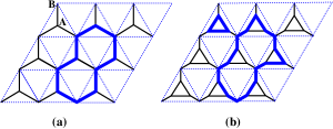
Figure 1: (Color online) The O($n$) loop model on the honeycomb lattice (a) and the martini lattice (b).

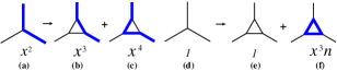
Figure 2: (Color online) Mapping of the vertex configurations. The weights of the different vertices are shown. The same weights apply to versions rotated by $\pm 2\pi/3$.

Consider a honeycomb lattice with two sublattices $A$ and $B$. A loop configuration $\cal G$ also denotes the occupations of sublattice $A$, as shown in Fig. 1(a). We rewrite the partition function (1) in the following way:

$$Z_{h} = \sum\limits_{\cal G}x^{v}n^{l}=\sum\limits_{\cal{\cal G}}(x^{2})^{v_{A}}1^{V_{A}-v_{A}}n^{l},$$ (5)

where $v=b$ is the number of vertices visited by loop segments, $V_{A}$ and $v_{A}=v/2$ are the number of vertices and the number of visited vertices of sublattice $A$, respectively. Thus the weight of a visited $A$ vertex shown in Fig. 2(a) is $x^{2}$, the weight of an empty $A$ vertex shown in Fig. 2(d) is 1.

Now consider the O($n$) loop model on the martini lattice, which is constructed by replacing the ‘star’ (an $A$ vertex) shown in Fig. 2(d) by the structure shown in Fig. 2(e). Each occupied (empty) $A$ vertex corresponds to two possible occupations on that structure, as shown in Fig. 2 (b) and (c) ((e) and (f)). Thus, any given configuration $\cal G$ of loops on the honeycomb lattice maps to the sum of $2^{V_{A}}$ possible loop configurations on the martini lattice. Let $x$ be the weight of a bond for the martini loop model, the partition function of the loop model on the martini lattice can be obtained by summing on $\cal G$:

$$Z_{m} = (1+x^{3}n)^{V_{A}}\sum\limits_{\cal G}(\frac{x^{3}+x^{4}}{1+x^{3}n})^{v_{A}}n^{l}.$$ (6)

Mapping $(x^{3}+x^{4})/(1+x^{3}n)\to x^{2}$, we obtain $Z_{h}$ in (5) multiplied by a trivial factor. It follows the critical points $x_{c}$ of the O($n$) loop model on the martini lattice

$$\frac{{x_{c}}^{3}+{x_{c}}^{4}}{1+{x_{c}}^{3}n}=\frac{1}{2+\sqrt{2-n}}.$$ (7)

This result is in agreement with an existing result for the O(1) loop model, which is equivalent to the high temperature expansion of the Ising model model baxter with $x={\rm tanh}K^{I}$, where $K^{I}$ is the coupling of Ising spins sitting on the vertices of the martini lattice. According to (7), $K^{I}_{c}=0.749790959036\cdots$, which coincides with the exactly known critical point of the $q=2$ Potts model on the martini lattice qAC .

As another special case, we present the exact connective constant of the SAW on the martini lattice. The substitution $\mu=1/x_{c}$ in (7) for $n=0$ determines $\mu$ as the solution of

$$\frac{1}{\mu^{3}}+\frac{1}{\mu^{4}}=1-\frac{\sqrt{2}}{2},$$ (8)

which yields $\mu=1.750564567897\cdots$.

We may further generalize above results by allowing bonds on the small triangles in Fig. 2(e) have weight ($x_{t}$) different from those on the remaining ones ($x_{s}$). Following the mapping described above, we thus obtain a critical line in the $x_{t}$ versus $x_{s}$ plane for a given $n$:

$$\frac{{x_{s}}^{2}x_{t}+{x_{t}}^{2}{x_{s}}^{2}}{1+{x_{t}}^{3}n}=\frac{1}{2+\sqrt{2-n}}.$$ (9)

For the 3-12 lattice, the critical line of the generalized model is

$$\frac{x_{s}(x_{t}+x_{t}^{2})}{1+x_{t}^{3}n}=\frac{1}{\sqrt{2+\sqrt{2-n}}}.$$ (10)

Finite-size scaling and transfer matrix calculation. Consider the lattice (the 3-12 or the martini lattice) wrapped on a cylinder with circumference $L$. The magnetic correlation function of the O($n$) spin model is translated as the probability that two sites at a distance $r$ are linked by a single loop segment cg , $g_{r}=Z^{\prime}/Z$, where $Z^{\prime}=\sum_{{\cal G}^{\prime}}x^{b}n^{l}$, and ${\cal G}^{\prime}$ denotes the configurations that connect sites 0 and $r$ by precisely one single loop segment. In our transfer-matrix analysis of the finite-size-scaling behavior, it is sufficient to substitute the configurations ${\cal G}^{\prime}$ that connect any site of row 0 to any site of a row at a distance $r$ as measured in the length direction of the cylinder. The exponential decay of $g_{r}$ at large distances is determined by the magnetic gap in the eigenvalue spectrum of the transfer matrix. The scaled magnetic gap $X_{h}(x,L)=\frac{L\zeta}{2\pi}\ln({\Lambda^{(0)}}/{\Lambda^{(1)}}),$ where $\Lambda^{(0)}$ and $\Lambda^{(1)}$ is the largest eigenvalue of the TM for $Z$ and $Z^{\prime}$, respectively. $\zeta$ is a geometrical factor determined by the ratio between the unit of $L$ and the thickness of a row added by the transfer matrix. Another scaled gap $X_{t}(x,L)=\frac{L\zeta}{2\pi}\ln({\Lambda^{(0)}}/{\Lambda^{(2)}})$, describes the exponential decay of the energy-energy correlation, with $\Lambda^{(2)}$ the second eigenvalue of the TM for $Z$.

The TM techniques of the O($n$) loop model are well described in the literature, e.g., see on . The procedure of sparse matrix decomposition for the martini and the 3-12 lattice equals to that for the honeycomb lattice with the adding units suitably chosen hycONTM . For further details, see pottsTM ; TM1 .

According to the finite-size scaling fss and the conformal invariance conformal theory, the scaled gap $X_{i}(x,L)$, in the vicinity of the critical point, satisfies

$$X_{i}(x,L)=X_{i}+a(x-x_{c})L^{y_{t}}+buL^{y_{u}}+\cdots,$$ (11)

where $X_{i}(i=h,t)$ is the magnetic and the temperature scaling dimension, respectively; $y_{t}$ is the thermal exponent; $u$ denotes the leading irrelevant field, $y_{u}$ is the associated irrelevant exponent. $a,b$ are unknown constants. Such behavior is illustrated in Fig. 3(a) and (c) for the case $n=0$. The critical point is estimated by numerically solving $x$ in the equation $X_{h}(x,L)=X_{h}(x,L-1)$, with system sizes up to $L=16$. The solution $x_{c}(L)$ converges to the critical value $x_{c}$ as

$$x_{c}(L)=x_{c}+a^{\prime}uL^{y_{u}-y_{t}}+\cdots,$$ (12)

where $a^{\prime}$ is an unknown constant. The numerical estimations and the theoretical predictions of the critical points of the martini lattice are listed in Table 1. Our numerical estimations coincide with the theoretical predictions in $9$ decimal numbers.

Table 1: Critical points $x_{c}$, conformal anomaly $c$, magnetic and temperature scaling dimensions $X_{h},X_{t}$ of the two-dimensional O($n$) loop model on the martini lattice. (T=Theoretical prediction, N=Numerical estimation.)

$n$	$x_{c}$(T)	$x_{c}$(N)	$c$(T)	$c$(N)	$X_{h}$(T)	$X_{h}$(N)	$X_{t}$(T)	$X_{t}$(N)
0	0.571244285	0.571244285(1)	0	0	0.1041667	0.104166(1)	2/3	0.666668(2)
0.25	0.584248605	0.584248605(1)	0.1300704	0.1300705(2)	0.1100192	0.1100193(1)	0.7395254	0.739526(1)
0.5	0.598867666	0.59886768(2)	0.2559499	0.255950(1)	0.1154420	0.1154420(1)	0.8177559	0.817756(1)
0.75	0.615559079	0.6155590(1)	0.3788781	0.3788783(3)	0.1204452	0.1204452(1)	0.9035105	0.9035104(2)
1.0	0.635024224	0.63502422(1)	0.5	0.500000(1)	0.125	0.12500000(1)	1	1.00000(1)
1.25	0.658437850	0.65843786(1)	0.6205051	0.6205053(2)	0.1290128	0.1290127(1)	1.1126008	1.1126007(1)
1.5	0.688067393	0.68806739(2)	0.7418425	0.741842(1)	0.1322435	0.1322434(1)	1.2518912	1.25189(1)
1.75	0.729662053	0.729664(3)	0.8662562	0.8662563(1)	0.1339623	0.13396(1)	1.4457176	1.445718(1)
2.0	0.840896415	-	1	1.000000(1)	0.125	0.1250000(1)	2	2.00000(1)

The universal values of $X_{i}$ and the conformal anomaly $c$ of the two-dimensional O($n$) loop model are exactly known as cg ; conformal

$$c = 1-\frac{6(g-1)^{2}}{g},$$

$$X_{h} = 1-\frac{1}{2g}-\frac{3g}{8},\ \ X_{t}=\frac{4-2g}{g},$$ (13)

where $n=-2\cos(\pi g)$, $1\leq g\leq 2$.

At criticality, $X_{i}(L)$ converges as follows to $X_{i}$ with increasing system size $L$

$$X_{i}(L)=X_{i}+b^{\prime}L^{y_{u}}+\cdots,$$ (14)

where $b^{\prime}$ is an unknown constant. The free energy density $f(L)=\zeta\ln\Lambda^{(0)}_{L}/L$ scales as BCN ; Affleck

$$f(L)=f(\infty)+\frac{\pi c}{6L^{2}}.$$ (15)

We then calculate $f(L),~{}X_{t}(L)$ and $X_{h}(L)$ for a sequence of systems up to size $L=16$ at the critical points (7). Fitting the data according to (14) and (15), we obtain the scaling dimensions $X_{h},~{}X_{t}$ and the conformal anomaly $c$, which are also listed in Table 1. Our numerical estimations are in agreement with the theoretical predictions with a high accuracy. For $X_{h},X_{t}$, our results are also consistent with the Monte Carlo results for $n\geq 1$ honeycombMC ; ONpercolation .

When $n$ approaches 2, $y_{t}=2-X_{t}\rightarrow 0$. The corrections to scaling due to the leading irrelevant field become relatively strong. At $n=2$, $y_{t}$ is exactly $0$, so that intersecting points between the curves $X_{i}(x,L)$ and $X_{i}(x,L-1)$ may be absent, as already suggested by (11), and as indeed observed in Fig. 3(b) and (d). Therefore, we can’t numerically determine the critical point $x_{c}$ in the usual way. However, $c$ and $X_{h},X_{t}$ are still estimated at the theoretical critical point.

Similar analysis is also performed to the 3-12 lattice. Theoretical predictions and numerical estimations of critical points for several values of $n$, which agree in a high accuracy, are listed in Table 2. ¿From Tables 1 and 2, we can see that the values of $X_{h},X_{t}$ and $c$ for a two-dimensional O($n$) loop model on the martini lattice coincide with those of the 3-12 lattice, as expected by the hypothesis of universality.

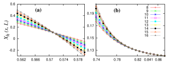
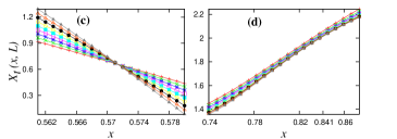
Figure 3: (Color online) Scaled gaps $X_{h}(x,L),X_{t}(x,L)$ versus $x$ for the O($n$) loop model on the martini lattice with $L$=8 to 16. (a) and (c): $n=0$; (b) and (d): $n=2$, with $x_{c}=0.840896$ indicated. Lines connecting data points are added to guide the eye.

Table 2: Critical points $x_{c}$, conformal anomaly $c$, magnetic and temperature scaling dimensions $X_{h},X_{t}$ of the two-dimensional O($n$) loop model on the 3-12 lattice. (T=Theoretical prediction, N=Numerical estimation.)

$n$	$x_{c}$(T)	$x_{c}$(N)	$c$(T)	$c$(N)	$X_{h}$(T)	$X_{h}$(N)	$X_{t}$(T)	$X_{t}$(N)
0	0.584439429	0.584439429(1)	0	0	0.1041667	0.104167(1)	2/3	0.666668(1)
0.25	0.601034092	0.601034092(1)	0.1300704	0.1300705(2)	0.1100192	0.1100193(1)	0.7395254	0.739526(1)
0.5	0.620240607	0.62024060(1)	0.2559499	0.255950(3)	0.1154420	0.115442(1)	0.8177559	0.817756(1)
0.75	0.642967899	0.6429678(1)	0.3788781	0.3788783(2)	0.1204452	0.1204452(1)	0.9035105	0.903510
1.0	0.670697664	0.67069766(1)	0.5	0.499999(1)	0.125	0.1250000(1)	1	1.000000(1)
1.25	0.706102901	0.70610291(1)	0.6205051	0.620505(1)	0.1290128	0.1290127(1)	1.1126008	1.112600(1)
1.5	0.754845016	0.754845(1)	0.7418425	0.741842(1)	0.1322435	0.1322435(1)	1.2518912	1.25189(1)
1.75	0.833205232	0.83320(2)	0.8662562	0.86626(1)	0.1339623	0.13396(1)	1.4457176	1.445718(2)
2.0	1.172534677	-	1	0.999999(1)	0.125	0.1250000(1)	2	2.00000(1)

Conclusion. We derived the exact critical points of the O($n$) loop model on the martini lattice, and performed a finite-size scaling analysis based on numerical TM calculations. Our numerical estimations agree with the theoretical predictions, within a margin that is typically of order $10^{-9}$. This rather high precision may be related to the vanishing of the leading irrelevant field in the Nienhuis result onhoneycomb for the critical line.

In the limit $n\to 0$, the critical point gives the exact connective constant $\mu=1.7505....$ of the SAWs on the martini lattice.

The exact critical points of the O($n$) loop model on the 3-12 lattice derived by Batchelor are also verified.

The conformal anomaly, the magnetic and the temperature scaling dimensions of the O($n$) models on the two lattices are numerically calculated. The estimations coincide with the theoretical predictions, as expected according to the universality hypothesis.

Acknowledgment. We thank Prof. F. Y. Wu and Prof. H. W. J. Blöte for a critical reading of the manuscript and valuable suggestions. This work is supported by the NSFC under Grant No. 11175018, the NCET-08-0053 and the HSCC of Beijing Normal University.

References

- (1) E. Domany, D. Mukamel, B. Nienhuis and A. Schwimmer, Nucl. Phys. B 190, 279 (1981).
- (2) H. E. Stanley, in Phase Transitions and Critical phenomena, edited by C. Domb and M. S. Green (Academic, London, 1987), Vol. 3.
- (3) B. Nienhuis, in Phase Transitions and Critical phenomena, edited by C. Domb and J. Lebowitz (Academic, London, 1987), Vol. 11.
- (4) B. Nienhuis, Phys. Rev. Lett. 49, 1062 (1982).
- (5) R. J. Baxter, J. Phys. A 19, 2821 (1986).
- (6) M. T. Batchelor and H. W. J. Blöte, Phys. Rev. Lett. 61, 138 (1988); Phys. Rev. B 39, 2391 (1989).
- (7) M. T. Batchelor, B. Nienhuis, and S. O. Warnaar, Phys. Rev. Lett. 62, 2425 (1989).
- (8) Y. M. M. Knops, B. Nienhuis, and H. W. J. Blöte, J. Phys. A 31, 2941 (1998).
- (9) H. W. J. Blöte and B. Nienhuis, J. Phys. A: Math. Gen. 22, 1415 (1989).
- (10) B. Li, W.-A. Guo, and H. W. J. Blöte, Phys. Rev. E 78, 021128 (2008).
- (11) P. G. de Gennes, Phys. Lett. A 38, 339 (1972).
- (12) B. Duplantier, J. Stat. Phys. 54, 581 (1989).
- (13) J. M. Hammersley, Proc. Camb. Phil. Soc. 53, 642 (1957).
- (14) P. J. Flory, J. Chem. Phys. 17, 303 (1949).
- (15) S. E. Alm, J. Phys. A 38, 2055 (2005).
- (16) M. E. Fisher and M. F. Sykes, Phys. Rev. 114, 45 (1959).
- (17) I. Jensen, J. Phys. A 37, 11521 (2004).
- (18) I. Jensen and A. J. Guttmann, J. Phys. A 31, 8137 (1998).
- (19) S. E. Alm and R. Parviainen, J. Phys. A 37, 549 (2004).
- (20) H. W. J. Blöte and B. Nienhuis, Physica A 160, 121 (1989).
- (21) Y. J. Deng, T. M. Garoni, W.-A. Guo, H. W. J. Blöte and A. D. Sokal, Phys. Rev. Lett. 98, 120601 (2007).
- (22) M. T. Batchelor, J. Stat. Phys. 92, 1203 (1998).
- (23) C. R. Scullard, Phys. Rev. E 73, 016107 (2006).
- (24) R. B. Potts, Proc. Cambridge Philos. Soc. 48, 106 (1952).
- (25) F. Y. Wu, Rev. Mod. Phys. 54, 235 (1982).
- (26) F. Y. Wu, Phys. Rev. Lett. 96, 090602 (2006).
- (27) R. J. Baxter, Exactly Solved Models in Statistical Mechanics (Academic, London, 1982).
- (28) H. W. J. Blöte and M. P. Nightingale, Physica A 112, 405 (1982).
- (29) H. W. J. Blöte and M. P. Nightingale, Phys. Rev. B 47, 15046 (1993).
- (30) For reviews, see e.g. M. P. Nightingale in Finite-Size Scaling and Numerical Simulation of Statistical Systems, ed. V. Privman (World Scientific, Singapore 1990), and M. N. Barber in Phase Transitions and Critical Phenomena, Vol. 8, eds. C. Domb and J. L. Lebowitz (Academic, New York 1983).
- (31) J. L. Cardy, J. Phys. A 17, L385 (1984).
- (32) H. W. J. Blöte, J. L. Cardy, and M. P. Nightingale, Phys. Rev. Lett. 56, 742 (1986).
- (33) I. Affleck, Phys. Rev. Lett. 56, 746 (1986).
- (34) C. X. Ding, Y. J. Deng, W.-A. Guo and H. W. J. Blöte, Phys. Rev. E 79, 061118 (2009).