Numerical and analytical investigation of the free boundary confluence for the phase field system.

Abstract

In this paper we numerically research the solutions of the phase field system for the spherically symmetric Stefan-Gibbs-Thomson problem in the case of interaction of the free boundaries. We analyze the effect of the soliton type disturbance of the temperature in the point of the contact of the free boundaries.

1 INTRODUCTION. STATEMENT OF THE PROBLEM

The main goal of this paper is the numerical research of the effect of the soliton type disturbance of the temperature in the point of the contact of the free boundaries. This effect we consider in the case of the phase field model for the Stefan-Gibbs-Thomson problem. The difference between this problem and the classical Stefan problem is that the surface tension is taken into account in the Stefan-Gibbs-Thomson problem. At the beginning of the paper we briefly give the main analytic results about the confluence of the free boundaries and then we illustrate these results by computer simulation.

The effect of the soliton type (negative) disturbance of the temperature $\sigma$ of the free boundaries in the point of the contact is shown in Fig. 1.

We present the results of the computer simulation for the phase field system in the spherically symmetric case. Namely, we consider the domain $Q=\Omega\times[0,t_{1}]$, where $\Omega=[R_{1},R_{2}]$ is the spherical layer in the spherical coordinates. We assume that the domain $\Omega$ is divided into the three layers $\Omega^{+}_{1,2}(t)$ and $\Omega^{-}(t)$ as follows:

$$\Omega^{+}_{1}(t)=[R_{1},r_{1}(t)],\quad\Omega^{-}(t)=[r_{1}(t),r_{2}(t)],\quad\Omega^{+}_{2}(t)=[r_{2}(t),R_{2}],$$

where $r_{i}(t)=\Gamma_{i}(t)$, $i=1,2$ is the free boundaries between phases ”$+$” and ”$-$”. We assume that the phase ”$+$” occupies the layer $\Omega^{+}_{1,2}(t)$, and the phase ”$-$” occupies the layer $\Omega^{-}(t)$ (see Fig. 2).

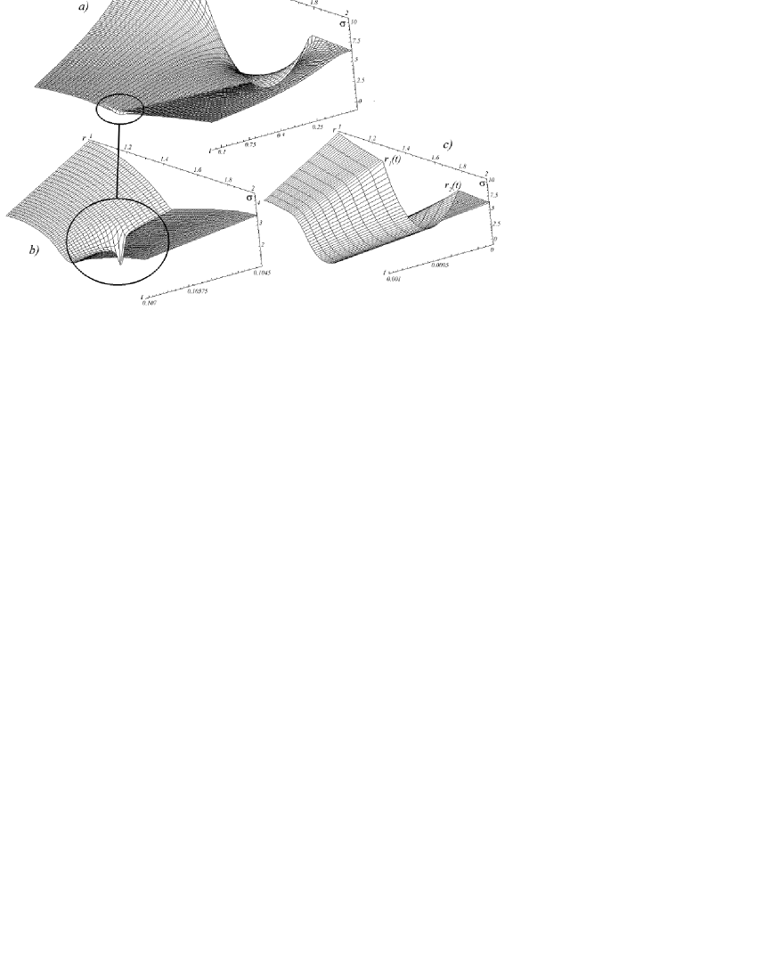
Figure 1: Effect of the soliton type disturbance of the temperature ($\varepsilon=0.003$). a) Coordinate and time dependence of the temperature. b) Soliton type disturbance of the temperature in the neighborhood of the point of the contact of the free boundaries. c) Initial data of the temperature and the evolution of the free boundaries $r_{1}(t)$, $r_{2}(t)$ in prime.

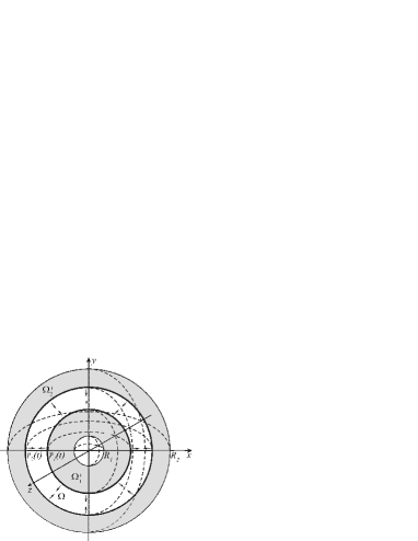
Figure 2: The free boundaries in the spherically symmetric case.

In this case the phase field system have the form [1]

$$L\theta=-\frac{\partial u}{\partial t},\qquad\varepsilon Lu-\frac{u-u^{3}}{\varepsilon}-\varkappa\theta=0,$$ (1)

where $\varkappa=\sqrt{2}/3$,

$$L=\frac{\partial}{\partial t}-\frac{1}{r^{2}}\frac{\partial}{\partial r}\left(r^{2}\frac{\partial}{\partial r}\right),\qquad r\in[R_{1},R_{2}],\quad t\in[0,t_{1}].$$

The function $\theta=\theta(r,t,\varepsilon)$ has the meaning of the temperature, and the function $u=u(r,t,\varepsilon)$ (so-called the order function) determines the phase state of the medium. Namely, the value $u\simeq-1$ corresponds to the phase ”$-$” in the layer $\Omega^{-}(t)$, and the value $u\simeq 1$ corresponds to the the phase ”$+$” in the layers $\Omega^{-}_{1,2}(t)$.

We denote

$$\theta(r,t)=\frac{\sigma(r,t)}{r}.$$ (2)

The phase field system (1) we can write in the form

$$\frac{\partial\sigma}{\partial t}-\frac{\partial^{2}\sigma}{\partial r^{2}}=-r\frac{\partial u}{\partial t},$$ (3)

$$\varepsilon Lu=\frac{u-u^{3}}{\varepsilon}+\varkappa\frac{\sigma}{r}.$$ (4)

Passing to the limit as $\varepsilon\to 0$ in (3), (4) we obtain the Stefan-Gibbs-Thomson problem for the each free boundary (see [1, 2, 6])

$$\frac{\partial\overline{\sigma}}{\partial t}=\frac{\partial^{2}\overline{\sigma}}{\partial r^{2}},\qquad r\in[R_{1},R_{2}],\quad r\neq\hat{r}_{i}(t),\quad i=1,2,$$ (5)

$$\left.\frac{\overline{\sigma}}{r}\right|_{r=\hat{r}_{i}(t)}=(-1)^{i+1}\left(\hat{r}_{i}^{\prime}(t)+\frac{2}{\hat{r}_{i}(t)}\right),$$ (6)

$$\left.\left[\frac{\partial\overline{\sigma}}{\partial r}\right]\right|_{r=\hat{r}_{i}(t)}=(-1)^{i+1}2\hat{r}_{i}(t)\hat{r}^{\prime}_{i}(t).$$ (7)

This passage to the limit is possible, for example, in the case where the corresponding limit problems have classical solutions. In this case, the weak limits as $\varepsilon\to 0$ of solutions (3), (4) give these solutions [1, 2, 6]. The existence of the classical solution $\overline{\sigma}$ of problem (5)–(7) is discussed in [8].

By $t^{*}\in(0,t_{1})$ we denote the instant of time of the confluence of the free boundaries, and $r^{*}=\hat{r}_{1}(t^{*})=\hat{r}_{2}(t^{*})$ is the sphere of the contact of the free boundaries.

The smooth approximations (i.e. the approximate solution of the system (3), (4) with misalignment that is small in the weak sense as $\varepsilon\to 0$, see [2]) of the Stefan-Gibbs-Thomson problem (of the phase field system) is constructed in [3] in the one dimensional case and this smooth approximations exists in the time included the instant of the contact $t^{*}$. Moreover, this smooth approximations is constructed on the assumption of the existence of the classical solution of the limit problem as $t\leqslant t^{*}-\delta$, where $\delta>0$ is any number. This approximations admits the passage to the limit as $\varepsilon\to 0$.

It is possible to show [2] that in the common sense the asymptotic solution of the system (3), (4) has the form

$$\sigma^{as}_{\varepsilon} =\bar{\sigma}^{-}(r,t)+\left(\bar{\sigma}^{+}(r,t)-\bar{\sigma}^{-}(r,t)\right)\omega_{1}\left(\frac{\hat{r}_{2}(t)-r}{\varepsilon}\right)\omega_{1}\left(\frac{r-\hat{r}_{1}(t)}{\varepsilon}\right),$$ (8)

$$u^{as}_{\varepsilon} =1+\omega_{0}\left(\frac{\hat{r}_{1}(t)-r}{\varepsilon}\right)$$ (9)

$$\qquad+\omega_{0}\left(\frac{r-\hat{r}_{2}(t)}{\varepsilon}\right)+\varepsilon\left[\frac{\sigma^{as}_{\varepsilon}}{2}+\omega\left(t,\frac{r-\hat{r}_{1}(t)}{\varepsilon},\frac{r-\hat{r}_{2}(t)}{\varepsilon}\right)\right].$$

as $t\leqslant t^{*}-\delta$, $\delta>0$. Here $\omega_{1}(z)\to 0,1$ as $z\to\mp\infty$, $\omega^{(k)}_{1}(z)\in\mathbb{S}(\mathbb{R}^{1}_{z})$ as $k>0$, $\hat{r}_{i}(t)$, $i=1,2$ is the smooth functions, $r_{1}\leqslant r_{2}$, $\omega_{0}(z)=\tanh(z)$, and $\omega(t,z_{1},z_{2})\in C^{\infty}([0,t^{*}];\,\mathbb{S}(\mathbb{R}^{2}_{z}))$. By $\mathbb{S}(\mathbb{R}^{n})$ we denote the Schwartz space of smooth rapidly decreases functions. If the initial data for (3), (4) has the form (8), (9) at $t=0$, then, for $t\leqslant t^{*}-\delta$, we have the estimate

$$\|u-u^{as}_{\varepsilon};C(0,T;L^{2}(\mathbb{R}^{1})\|+\|\sigma-\sigma^{as}_{\varepsilon};\mathcal{L}^{2}(Q)\|\leqslant c\varepsilon^{\mu},\qquad\mu\geqslant 3/2,$$

where $(\sigma,u)$ is a solution of system (3),(4) (see [2] and references in). Here $Q=\Omega\times[0,t^{*}-\delta]$, and the constant $c$ is independent of $\varepsilon$.

The main obstacle to the construction of approximations of solution in the case of confluence of free boundaries is the fact that, instead of an ordinary differential equation whose solution is the function $\omega_{0}(z)$ [1, 2], in the case of confluence of free boundaries, we must deal with a partial differential equation for which the explicit form of the exact solution is unknown.

In papers [3, 4] using the the weak asymptotic method the solution of the phase field system was constructed that describes the confluence of the free boundaries. Namely, the ansatz of the order function has the form.

$$\check{u} =\frac{1}{2}\left[1+\omega_{0}\left(\beta\frac{r_{1}^{2}-r^{2}}{\varepsilon}\right)+\omega_{0}\left(\beta\frac{r^{2}-r_{2}^{2}}{\varepsilon}\right)\right.$$ (10)

$$-\left.\omega_{0}\left(\beta\frac{r_{1}^{2}-r^{2}}{\varepsilon}\right)\omega_{0}\left(\beta\frac{r^{2}-r_{2}^{2}}{\varepsilon}\right)\right].$$

The temperature is sought in the form

$$\check{\sigma}=e(r)\check{T}+q,$$ (11)

$e(r)\in C_{0}^{\infty}([R_{1},R_{2}])$, $e\equiv 1$ for $r\in[\hat{r}_{1}(0),\hat{r}_{2}(0)]$. Here $\check{T}$ is the model of the temperature, i.e. it is the function of the simplest structure which describes the behaviors of the temperature qualitatively correct, and $q$ is an unknown smooth function. Namely,

$$\check{T} =\gamma_{1}^{+}(t)(r_{1}-r)H(r_{1}-r)+\gamma_{2}^{+}(t)(r-r_{2})H(r-r_{2})$$

$$+\gamma^{-}(r,t)\frac{(r_{1}-r)(r-r_{2})}{r_{2}-r_{1}}H(r-r_{1})H(r_{2}-r)$$ (12)

$$+\hat{\gamma}(r,t)\frac{(r_{1}-r)(r-r_{2})}{r_{2}-r_{1}}H(r_{1}-r)H(r-r_{2})+I(r,t).$$

Here

$$\gamma^{-}=\frac{\gamma_{1}^{+}-\gamma_{2}^{-}}{2}-(r^{2}-r^{*2})\frac{\gamma_{1}^{+}+\gamma_{2}^{-}}{\psi}$$

$$\hat{\gamma}=\frac{\hat{\gamma}_{1}+\hat{\gamma}_{2}}{2}-(r^{2}-r^{*2})\frac{\hat{\gamma}_{1}-\hat{\gamma}_{2}}{\psi},\qquad r^{*}=\frac{\sqrt{r_{1}^{2}+r_{2}^{2}}}{2}.$$

$$I=\frac{k_{1}-k_{2}}{2}-(r^{2}-r^{*2})\frac{k_{1}+k_{2}}{\psi},\quad k_{1}=r_{1}r_{1t}+2,\quad k_{2}=r_{2}r_{2t}+2,$$ (13)

$$\psi(t,\varepsilon)=r_{2}^{2}(t,\varepsilon)-r_{1}^{2}(t,\varepsilon),$$ (14)

So, from the given above formulas we see that the model $\check{T}$ is linear in $r$ in the layers $\Omega^{+}_{i}(t)$, $i=1,2$ and parabolic in $r$ in the layer $\Omega^{-}(t)$.

In paper [3] the formulas are obtained those determine the functions contained in ansatzes (10), (11) in the one dimensional case.

The analysis of these formulas shows that the contained in the phase field system temperature $\theta$ has the soliton type disturbance in the neighborhood of the point of the contact. This disturbance is localized in the space coordinates and in time. The ”width” of this localization is proportional to $\varepsilon$. In [3] the limit as $\varepsilon\to 0$ of the amplitude of the disturbance is derived. In the one dimensional case the value of this amplitude is given by formula

$$\left.\left[\bar{\theta}\right]\right|_{x=x^{*},\ t=t^{*}}=-\lim_{t\to t^{*}-0}\lim_{\varepsilon\to 0}\frac{V_{1}+V_{2}}{2},$$

where $V_{1}$ and $V_{2}$ are the velocities of the merging (one-dimensional) free boundaries.

The analytic treatment based on the weak asymptotics method shows that such effect is general. For example, the exactly same formula is correct in the case of merging globe layers [4] those is shown in Fig.2. Namely,

$$\left.\left[\bar{\theta}\right]\right|_{r=r^{*},\ t=t^{*}}=-\lim_{t\to t^{*}-0}\lim_{\varepsilon\to 0}\frac{V_{1n}+V_{2n}}{2},$$

$V_{1n}$ and $V_{2n}$ are the normal velocities of the merging three-dimensional free boundaries (correspondingly, $\Gamma_{1}(t)$ and $\Gamma_{2}(t)$). If the free boundaries are asymmetrical, then their principle curvatures have the like signs at the point of the contact. In this case the amplitude of the jump of the temperature is determined by formula

$$\left.\left[\bar{\theta}\right]\right|_{(x,y,z)=(x^{*},y^{*},z^{*}),\ t=t^{*}}=-\lim_{t\to t^{*}-0}\lim_{\varepsilon\to 0}\left(\frac{|V_{1n}|+|V_{2n}|}{2}-|\mathcal{K}_{1}-\mathcal{K}_{2}|\right)$$

in the instant of the confluence and at the point of the contact. Here $\bar{\theta}=\bar{\theta}(x,y,z,t)$, $(x^{*},y^{*},z^{*})$ is the point of the contact of the free boundaries, and $\mathcal{K}_{1}$, $\mathcal{K}_{2}$ are the principle curvatures of the free boundaries at the point of the contact.

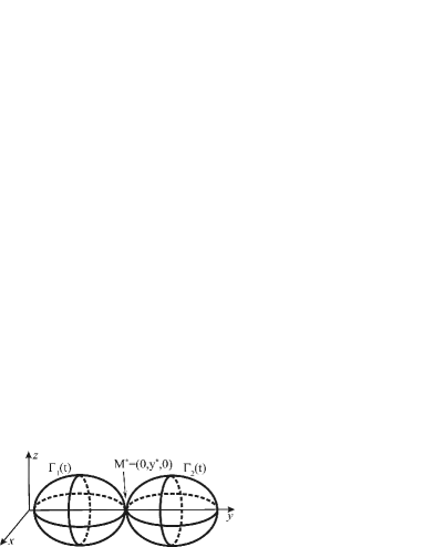
Figure 3: Confluence of the free boundaries in the case of the curvatures of the free boundaries have the unlike signs.

Let us consider another situation. We assume that the solution of our problem is symmetric about $y$-axe (see Fig.3). By $y_{1}(t)$ and $y_{2}(t)$ we denote the points in which the free boundaries cross the $y$-axe and these points is situated on the shorts distance one from another. We assume that $M^{*}=(0,y^{*},0)$ is the point of the contact of the free boundaries. The principle difference between this situation and the situation in Fig.2 is that in the instant of the contact $t^{*}$ the principle curvatures of the free boundaries have the unlike signs at the point of the contact $M^{*}$. In this case the amplitude of the jump of the temperature is determined by formula

$$\left.\left[\bar{\theta}\right]\right|_{(x,y,z)=(0,y^{*},0),\ t=t^{*}}=-\lim_{t\to t^{*}-0}\lim_{\varepsilon\to 0}\left(\frac{|V_{1n}|+|V_{2n}|}{2}+|\mathcal{K}_{1}|+|\mathcal{K}_{2}|\right).$$

The mentioned soliton type disturbance is observed in the numerical experiments, see Fig.9, 10.

We note that beside the our own papers we know only the single paper of A.M. Meirmanov and B.A. Zaltsman [7]. In this paper the problem of the confluence of the free boundaries in the case of the Hele-Shaw problem is derived and this problem is the special case of the Stefan-Gibbs–Thomson problem. The regularized (not limit) problem is considered in [7] and in this case the effect of the soliton type disturbance is not shown. The analog of this fact is the following problem. Let us consider the heat equation in a rectilinear segment and with not zero ($=1$) Dirichlet’s initial condition. Clearly, the solution of this problem is zero. However, the numerical solution is not identical zero for the different scheme with a node in the point $x=0$.

2 DIFFERENT SCHEME

The choice of the different scheme for system (3), (4) is based on some ideas that are sufficiently general for solving nonlinear equations. Namely, we calculate the heat equation (3) at the next time step and, consequently split system (3), (4). We associate Eq. (4) with implicit different scheme

$$\varepsilon u^{k+1}_{\bar{t}}-\varepsilon\sum_{i=1}^{n}u^{k+1}_{r_{i}\bar{r}_{i}}-2\varepsilon\sum_{i=1}^{n}\frac{u^{k+1}_{r_{i}}}{r_{i}}=$$ (15)

$$=\frac{1}{\varepsilon}\left[u^{k+1}-\left((u^{k})^{3}+3(u^{k})^{2}(u^{k+1}-u^{k})\right)\right]+\varkappa\sum_{i=1}^{n}\frac{\sigma^{k}_{i}}{r_{i}}.$$

Here $u^{k}$ is the mesh order function at the $k$-th time step, $\sigma^{k}$ is the mesh ”temperature” at the $k$-th time step.

The first term (the term in the square brackets) in the right hand part of Eq. (15) is obtained as following. We denote

$$F(u)=u-u^{3}.$$

We linearize the mesh function $F(u^{k+1})$ as following

$$F(u^{k+1})\approx F(u^{k})+F^{\prime}_{u}(u^{k})(u^{k+1}-u^{k}).$$

System (15) is completed with initial and boundary conditions in the points $r=R_{j}$, $j=1,2$. It is clear that Eqs. (15) is the three-point equations relatively to $u^{k+1}$ and these equations are solved by the sweep method.

To calculate the mesh ”temperature” $\sigma^{k+1}$ we use the standard different scheme for the heat equation (3). Namely,

$$\sigma_{\bar{t}}^{k+1}-\sum_{i=1}^{n}\sigma^{k+1}_{r_{i}\bar{r}_{i}}=-\sum_{i=1}^{n}r_{i}\sigma^{k+1}_{i\bar{t}}.$$ (16)

Equations (16) is also solved by the sweep method.

We use the main segment $r\in[1,2]$ (i.e., $R_{1}=1$, $R_{2}=2$) for the numerical simulation of the process of the confluence.

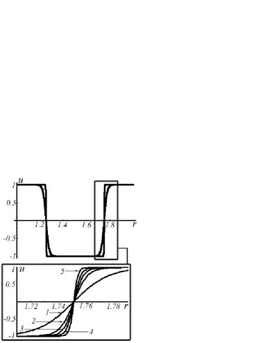
Figure 4: The initial data for the order function $u$ for the different values of $\varepsilon$: 1. $\varepsilon=0.025$, 2. $\varepsilon=0.01$, 3. $\varepsilon=0.007$, 4. $\varepsilon=0.005$, 5. $\varepsilon=0.003$.

The initial data we choose as provided by the structure of the weak asymptotic solution (9). We use the function

$$u^{0}=1+\tanh\left(\frac{r_{1}^{0}-r}{\varepsilon}\right)+\tanh\left(\frac{r-r_{2}^{0}}{\varepsilon}\right)$$ (17)

as the initial data for the order function $u$. Here $r_{1}^{0}=1.25$, $r_{2}^{0}=1.75$ determine the initial position of the free boundaries (see Fig.4,5).

The initial data $\sigma^{0}$ for the ”temperature” is taken in the form in Fig.5 as provided by model (1). Namely, the function $\sigma^{0}$ is parabolic in the domain with phase ”$-$” (between the free boundaries), and the function $\sigma^{0}$ is linear in the domain with phase ”$+$”. At the same time, the dependence between the initial positions and the initial velocities of the free boundaries and the values of $\sigma^{0}$ is determined by formula (6)in the boundary points $r_{1}^{0}$, $r_{2}^{0}$.

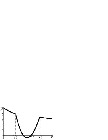
Figure 5: The initial data for the temperature $\sigma$. The initial positions of the free boundaries are $r_{1}^{0}=1.25$, $r_{2}^{0}=1.75$

It is clear that the considered initial data differ from the exact solution of the problem. Nevertheless it is known that the solutions of problem (3), (4) converge to solutions of the limit Stefan-Gibbs-Thomson problem as $\varepsilon\to 0$ and on the sufficiently general assumptions. More other, the solution of the Cauchi problem come to self-similar regime by the widely known behaviours of the semi-linear parabolic equations (see [5]). Beside it, the formulas for the asymptotic solution are the deformations of the formulas for the semi-similar solution.

3 THE RESULTS OF NUMERICAL SIMULATION

Let us consider the results of the numerical simulation of the process of the confluence of the free boundaries.

Some graphics given below illustrate the common behaviors of the solution of system (3), (4) and confirm the certainty of the numerical results. We simulate for the different (decreasing) values of the parameter $\varepsilon$, $\varepsilon=0.025$, $\varepsilon=0.01$, $\varepsilon=0.007$, 4. $\varepsilon=0.005$, $\varepsilon=0.003$. The mesh is equal $h=10^{-3}$ and the time step is equal $\tau=10^{-5}$.

In Fig.6, 7 are shown the profiles of the temperature $\sigma$ and the order function $u$ in the neighborhood of the point of the contact of the free boundaries (for fixed $r^{*}\approx r=1.42$) for different values of the parameter $\varepsilon$.

From the graphics in Fig.6 we see that the ”width” of the neighborhood of the instant of time of the jump of the temperature decrease (it is proportional to $\varepsilon$) owing to decreasing $\varepsilon$. At the same time, the jump occurs at the the different instant of time for the different values of the parameter $\varepsilon$. Namely, in dependence of the decreasing of $\varepsilon$ the sequence of the instant of time $t_{min}$ (in which the jump becomes minimum) increases, see also Table 1. Beside it, from Table 1 we see that the intervals grow short between the neighboring instants $t_{min}$ as the parameter $\varepsilon$ decreases. The cause of this fact is that the width of the transition zone of the order function $u$ is different for different values of $\varepsilon$, see formula (17). Namely, the width of transition zone is proportional $\varepsilon$ (as larger the value of $\varepsilon$, as wider the transition zone), see Fig. 4 and [1, 2]. As a result of this fact the contact of the transition zones (and, consequently the beginning of the confluence of the free boundaries) occurs previously for the simulation process with larger $\varepsilon$, see Fig. 8. Clearly, the width of the confluence is also proportional to $\varepsilon$ respect to $r$. From Fig. 8 we see that for the fixed instant of time $t=0.082$ the free boundaries corresponding to the graphic 1 ($\varepsilon=0.025$) complete the confluence, but at the same time the free boundaries corresponding another graphics (for smaller $\varepsilon$) are on the sufficiently large distance.

From Fig. 7 we see that as smaller $\varepsilon$ as quickly transit occurs from the phase ”$-$” to the phase ”$+$”. It is clear that $u(r^{*},t)\to\mathrm{sign}(t-t_{min})$ as $\varepsilon\to 0$.

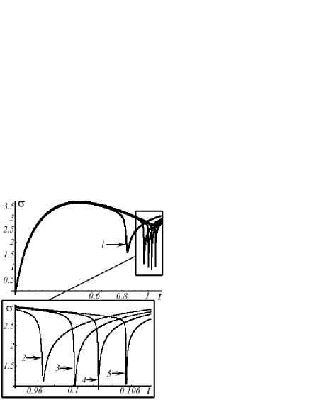
Figure 6: The jump of the temperature $\sigma$ in the neighborhood of the point of the contact of the free boundaries ($r^{*}\approx r=1.42$): 1. $\varepsilon=0.025$, 2. $\varepsilon=0.01$, 3. $\varepsilon=0.007$, 4. $\varepsilon=0.005$, 5. $\varepsilon=0.003$.

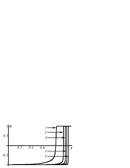
Figure 7: The order function $u$ in the neighborhood of the point of the contact of the free boundaries ($r^{*}\approx 1.42$): 1. $\varepsilon=0.025$, 2. $\varepsilon=0.01$, 3. $\varepsilon=0.007$, 4. $\varepsilon=0.005$, 5. $\varepsilon=0.003$.

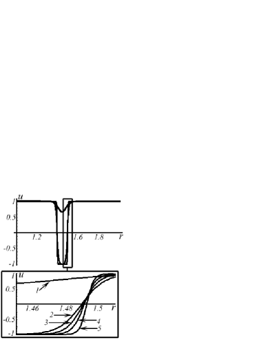
Figure 8: The order function $u$ at $t=0.082$: 1. $\varepsilon=0.025$, 2. $\varepsilon=0.01$, 3. $\varepsilon=0.007$, 4. $\varepsilon=0.005$, 5. $\varepsilon=0.003$.

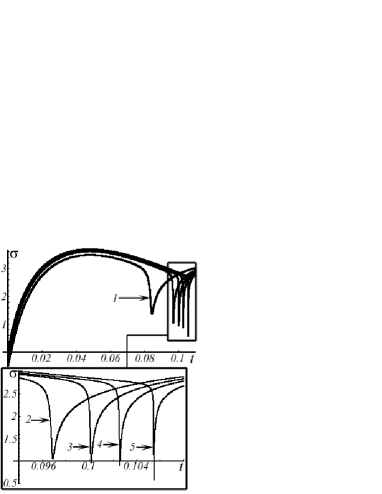
Figure 9: The jump of the temperature $\sigma$: 1. $\varepsilon=0.025$, $r=1.448$, 2. $\varepsilon=0.01$, $r=1.427$, 3. $\varepsilon=0.007$, $r=1.422$, 4. $\varepsilon=0.005$, $r=1.419$, 5. $\varepsilon=0.003$, $r=1.415$.

$\varepsilon$	$t_{min}$	$r_{min}$	$\sigma(r_{min},t_{min},\varepsilon)$
0.025	0.08432	1.448	1.373699
0.01	0.09690	1.427	1.051388
0.007	0.10016	1.422	0.967825
0.005	0.10260	1.419	0.902497
0.003	0.10549	1.415	0.587919

Table 1: Coordinate and time dependence of the jump of the temperature $\sigma$. $r_{min}$ and $t_{min}$ are values of the coordinate $r$ and time $t$ at which the jump becomes minimum.

Beside it, from Fig.6 we see that the minimum of the jump for the graphic 5 ($\varepsilon=0.003$) is smaller then the minimum of the jump for the graphic 4 ($\varepsilon=0.005$). But in real this is not true and we observe reversed dependence, see Table 1 and Fig.9. Here are shown the graphics of the temperature $\sigma$ in the fixed point $r=r_{min}$, where $r_{min}$ is the value of the coordinate $r$, in which the jump of the temperature becomes zero. This fact means that the shift of the minimum of the jump of the temperature $\sigma$ depend on $\varepsilon$ in the coordinate $r$, see Table 1. From Table 1 we see that this shift is not lager the difference between the width of the transition zones (difference between the the corresponding values of the parameter $\varepsilon$) for the corresponding graphics, see Fig.9.

From Table 1 we see that the intervals between the neighborhood values of $t_{min}$ decrease as $\varepsilon$ decreases. More other, this intervals is the order of $\varepsilon$. At the same time the distance between the neighborhood points $r_{min}$ grows short as $\varepsilon$ decreases.

The dynamic of the jump of the temperature at time is shown in Fig. 10 for $\varepsilon=0.003$.

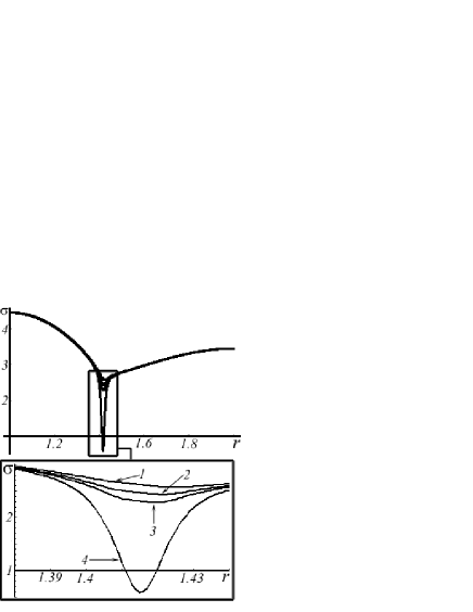
Figure 10: The dynamic of the jump of the temperature $\sigma$ for $\varepsilon=0.003$: 1. $t=0.1052$, 2. $t=0.10539$, 3. $t=0.10544$, 4. $t=t_{min}=0.10549$.

So we can conclude that the process of the confluence of the free boundaries is localized in the coordinate and at the time. Consequently, the soliton type disturbance of the temperature is localized in the coordinate and at the time (the width of the localization is proportional to$\varepsilon$), see Fig. 1.

We denote that the values of the parameter $\varepsilon>0.003$ is not possible in the our simulation. For $\varepsilon=0.003$ and $h=0.001$ we obtain that the three nodes (the minimal number of the nodes that necessary to calculate the second difference derivation, see) of the mesh appear in the transition zone, see (15), (16). The computer simulation shows that the numerical solution is unstable in the neighborhood of the confluence of the free boundaries for $\varepsilon=0.002$ and the different scheme do not give solution for $\varepsilon=0.001$.

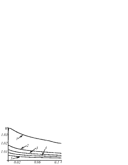
Figure 11: The order function $u$ in $r=1.15$: 1. $\varepsilon=0.025$, 2. $\varepsilon=0.01$, 3. $\varepsilon=0.007$, 4. $\varepsilon=0.005$, 5. $\varepsilon=0.003$.

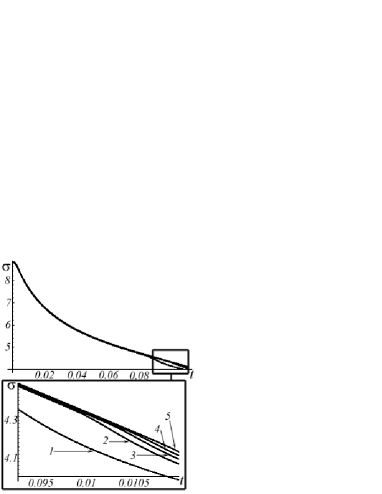
Figure 12: The temperature $\sigma$ in $r=1.15$: 1. $\varepsilon=0.025$, 2. $\varepsilon=0.01$, 3. $\varepsilon=0.007$, 4. $\varepsilon=0.005$, 5. $\varepsilon=0.003$.

The series of the graphics demonstrates the stability of the numerical solution of system (3), (4) respect to $\varepsilon$. In Fig.11, 12 are shown the graphics of the dependence of the order function $u$ and of the temperature $\sigma$ on time in the fixed point $r=1.15$. We note that the analogous results are correct for the another value of $r$ except the point of the contact of the free boundary.

From the graphics in Fig.11 we see that at the beginning ($t\leqslant 0.01$) the solution $u$ undergo the sharp jump and thereafter stables (undergo to near semi-similar regime). At the same time, this stabilization is wavelike. More other, the initial interval of the time in which the solution undergo the most strong change (jump) grows short as $\varepsilon$ decreases. More other the distance between the neighborhood graphics grows short as $\varepsilon$ decreases and this distance is proportional.

From the graphics in Fig.12 we see that the temperature $\sigma$ is stable respect to the variation of $\varepsilon$. For $t>0.09$ the difference between the graphics due to the process of the confluence for the graphics for the larger $\varepsilon$ begins early than for the graphics for the smaller $\varepsilon$.

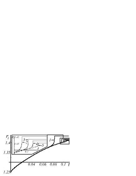
Figure 13: The dynamic of the free boundary $r_{1}(t)$ for the different values of the parameter $\varepsilon$: 1. $\varepsilon=0.025$, 2. $\varepsilon=0.01$, 3. $\varepsilon=0.007$, 4. $\varepsilon=0.005$, 5. $\varepsilon=0.003$.

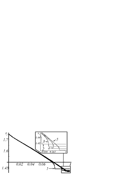
Figure 14: The dynamic of the free boundary $r_{2}(t)$ for the different values of the parameter $\varepsilon$: 1. $\varepsilon=0.025$, 2. $\varepsilon=0.01$, 3. $\varepsilon=0.007$, 4. $\varepsilon=0.005$, 5. $\varepsilon=0.003$.

The last series of the numerical experiments deals with the verification of the analytical formula for the amplitude of the jump of the temperature. Namely, in paper [4] is obtained the formula for the amplitude of the jump

$$\left.\left[\bar{\theta}\right]\right|_{r=r^{*},\ t=t^{*}}=-\frac{r_{10}^{\prime}-r_{20}^{\prime}}{2},$$

or taken into account (2) we have

$$\left.\left[\bar{\sigma}\right]\right|_{r=r^{*},\ t=t^{*}}=-\lim_{t\to t^{*}-0}\lim_{\varepsilon\to 0}\frac{2r_{1}(t,\varepsilon)r_{1}^{\prime}(t,\varepsilon)-2r_{2}(t,\varepsilon)r_{2}^{\prime}(t,\varepsilon)}{4}.$$ (18)

In Fig.13, 14 the dependence of the free boundaries $r_{1}(t)$ and $r_{2}(t)$ on time is shown for the different values of the parameter $\varepsilon$. We see that the functions $r_{1}(t)$ and $r_{2}(t)$ is linear in the initial interval of the shifting of the free boundaries. The nonlinearity of the confluence depends on the shifting of the free boundary near the point of the contact and the lines are distorted. We see that as smaller $\varepsilon$ as smaller the neighborhood of the instant $t^{*}$ in which the distortion is sensed.

The functions $r_{i0}(t)$, $i=1,2$ are determined as the limits

$$r_{i0}=\lim_{\varepsilon\to 0}r_{i}(t,\varepsilon)$$

in the asymptotic formulas. So in the capacity of $\frac{d}{dt}r_{i0}(t^{*})$ we should take the constants which are obtained by differentiation of the functions $r_{i}(t,\varepsilon)$ in the interval where this functions the most close to the line.

We note that the positions of the free boundaries is fuzzy respect to $\varepsilon$ as $\varepsilon>0$ (the width of the transition zone is proportional to $\varepsilon$). Therefore to disclose the behavior of the shifting the free boundaries we consider the dynamic of the point of the crossing the order function $u(r,t)$ and the axis $r$, i.e. we trace the dynamic of the points $r(t)$ in which $u(r(t),t)=0$ for any fixed $t$, see Fig.13, 14. The instants of time $t^{*}$ in which the graphics of $r_{1}(t)$ and $r_{2}(t)$ become the horizontal lines correspond to the instants of time in which the order function $u(r,t)$ becomes positive. This instants of time naturally do not equal to instants of time $t_{min}$ in which the amplitude of the jump of the temperature is maximal, see Table 1.

To calculate the amplitude of the jump of the temperature we determine the minimal value of the temperature $\sigma_{min}$ corresponded to the value of the coordinate $r_{min}$, see Table 1. For example in Fig. 10, this value of the coordinate is become on the curve 4. The amplitude is equal to the absolute value of the difference between $\sigma_{min}$ and the value of the temperature in the point $r_{min}$ and at the instant of time corresponded to the start of the fast changing of the temperature in this point (in Fig. 10 the curve 3 gives this value of the temperature).

The results of the verification of the formula (18) are showed in Table 2.

$\varepsilon$	$r_{1}$	$r^{\prime}_{1}$	$r_{2}$	$r^{\prime}_{2}$	$\left[\sigma_{an}\right]$	$\left[\sigma_{cal}\right]$
0.025	1.394	1.4	1.485	-3.2	3.01448	1.5
0.01	1.402	1	1.446	-3.2	3.3518	1.7
0.007	1.403	0.8	1.438	-3.2	2.86	1.9
0.005	1.403	0.6	1.430	-3.2	2.7	2.1
0.003	1.405	0.6	1.422	-3.2	2.69	2.7

Table 2: The value of the amplitude of the jump of the temperature $\sigma$ obtained by analytical formula ($\left[\sigma_{an}\right]$) and by numerical simulation ($\left[\sigma_{cal}\right]$).

In column $\left[\sigma_{an}\right]$ the data for the jump are given obtained by formula (2), and in column $\left[\sigma_{cal}\right]$ the data for the jump are given calculated by numerical simulation. From Table 2 we see that the analytical data converge to the numerical data as $\varepsilon$ decreases.

References

- [1] G.Caginalp An analysis of a phase field model of a free boundary. Arch. Rat. Mech. Anal. 92 (1986), 205–245.
- [2] V.G.Danilov, G.A.Omel’yanov & E.V.Radkevich Asymptotic solution of a phase field system and the modified Stefan problem. 1995, Differential’nie Uravneniya 31(3), 483–491 (in Russian).(English translation in Differential Equations 31(3), 1993.
- [3] V.G.Danilov Weak asymptotic solution of phase-field system in the case of confluence of free boundaries in Stefan problem with undercooling. Euro. Journ. Appl. Math. (2007) v.18, pp 537-569.
- [4] V.G.Danilov, V.Yu.Rudnev Confluence of the nonlinear waves in the Stefan–Gibbs-Thomson problem. Free boundary problems. To be published.
- [5] G.A.Omel’yanov and V.Yu.Rudnev Interaction of free boundaries in the modified Stefan problem. Nonlinear Phenomena in Complex Systems, 7:3 (2004) 227 - 237.
- [6] P.I. Plotnikov and V.N. Starovoitov Stefan problem as the limit of the phase field system., Differential Equations 29 (1993), 461–471.
- [7] A.Meirmanov, B.Zaltzman Global in time solution to the Hele-Shaw problem with a change of topology. EJAM, Vol. 13, pp. 431-447, 2002.
- [8] A.Meirmanov The Stefan Problem. Berlin . New York: Walter de Gruyter, 1992.