Dipolar Bose-Einstein condensate for large scattering length

Abstract

A uniform dilute Bose gas of known density has a universal behavior as the atomic scattering length tends to infinity at unitarity while most of its properties are determined by a universal parameter $\xi$ relating the energies of the noninteracting and unitary gases. The usual mean-field equation is not valid in this limit and beyond mean-field corrections become important. We use a dynamical model including such corrections to investigate a trapped disk-shaped dipolar Bose-Einstein condensate (BEC) and a dipolar BEC vortex for large scattering length. We study the sensitivity of our results on the parameter $\xi$ and discuss the possibility of extracting the value of this parameter from experimental observables.

I Introduction

The properties of a uniform dilute interacting $-$ Bose or Fermi $-$ atomic quantum gas interacting by an $S$-wave contact inteaction at zero temperature is determined by two scales $-$ the atomic scattering length $a$ and density $\bar{n}$. As $a\to\infty$ at unitarity, the first scale is not of concern and the observables of the gas are solely determined by density and the gas exhibits a universal behavior. Bulk chemical potential $\bar{\mu}$ of the unitary gas is proportional to the only available energy scale $-$ the Fermi energy (or the chemical potential of the noninteracting gas) $E_{F}=\hbar^{2}(6\pi^{2}\bar{n})^{2/3}/2m$ $-$ so that $\bar{\mu}=\xi E_{F}$, where $\xi$ is a universal parameter and $m$ is the mass of an atom rmp ; stoof ; ska ; skab ; feruni1 ; feruni2 ; feruni3 ; feruni4 ; feruni5 ; feruni6 ; feruni7 ; feruni8 ; bosuni1 ; bosuni2 ; bosuni3 ; bosuni4 . Similarly, the energy per particle $\bar{E}$ of the unitary gas is proportional to the energy per particle $E(\equiv 3E_{F}/5)$ of the noninteracting gas: $\bar{E}=\xi E$ feruni1 ; feruni2 . The Fermi energy is a physically meaningful quantity for the Fermi gas, but the same can also be used as an energy scale for the Bose gas stoof ; bosuni1 ; bosuni3 . The Bose and Fermi gases behave similarly at unitarity, because the Bose gas exhibits fermionization. If this fermionization of the Bose gas is absolute, then $\xi$ should be the same for the Bose and Fermi gases.

The parameter $\xi$ relating the energy of the noninteracting and unitary gases, has been “measured” experimentally from a study at or near unitarity of the density rmp ; feruni3 ; feruni4 ; feruni5 , or of ground-state energy, or of sound velocity feruni6 of a trapped Fermi gas. But a similar experiment is more difficult for a Bose-Einstein condensate (BEC) due to a large probability of three-body loss by molecule formation at or near unitarity, which is the threshold for molecule formation bosuni1 . In the weak-coupling limit ($an^{1/3}<1$) the mean-field Gross-Pitaevskii (GP) equation gives a good description of a trapped BEC, where $n$ is the density. In the strong-coupling regime ($an^{1/3}>1$) the GP equation highly overestimates the atomic contact interaction and leads to unphysical results. Experimental activities to access the strong-coupling regime of a BEC, to test the beyond mean-field corrections jila ; rice , and to extract the parameter $\xi$ from these studies have just began bosuni1 . Although unitarity is also the threshold for molecule formation in a two-component (spin up and down) Fermi gas, the probability of formation of diatomic molecules is highly suppressed in this case due to Pauli repulsion among spin-parallel fermions in the three-fermion system and hence is not of concern rmp .

Lately, BECs of ⁵²Cr cr1 ; cr2 and ¹⁶⁴Dy dy1 ; dy2 with large dipolar interaction have been observed and studied. The inter-atomic interaction now has two components: an $S$-wave contact interaction and an anisotropic long-range dipolar interaction. This allows to study the dipolar BEC with a variable contact interaction cr1 ; dy2 using a Feshbach resonance fesh . The intrinsically anisotropic dipolar BEC pla has many distinct features cr1 ; cr2 ; cr3 ; cr4 ; cr5 ; adhisol . The stability of a dipolar BEC depends not only on the scattering length, but also on the trap geometry cr1 ; cr3 ; cr5 . A disk-shaped trap leads to a repulsive dipolar interaction and the dipolar BEC is more stable, whereas a cigar-shaped trap yields an attractive dipolar interaction and hence favors a collapse instability cr1 ; cr5 ; cr6 .

We study the static and dynamic properties of a disk-shaped dipolar BEC and dipolar BEC vortex, with the dipole moments aligned perpendicular to the plane of the disk, for large scattering length using a beyond-mean-field model skab ; skab2 for the BEC-unitarity crossover. In this paper we consider the strong-coupling limit of the contact interaction only and not the same limit of dipolar interaction. In the weak-coupling limit, this crossover model reduces to the GP equation and the Lee-Huang-Yang (LHY) correction lhy , whereas in the strong-coupling regime of large scattering length it reduces to the universal result at unitarity. We find that the radial densities are sensitive to the parameter $\xi$ in the strong-coupling regime and hence a study of density is expected to yield information about this parameter. However, the frequency of oscillation of the dipolar BEC is found to be insensitive to this parameter. From a study of vortices in a disk-shaped dipolar BEC we find that both density and radius of vortex core are sensitive to this parameter in the strong-coupling regime.

In the disk configuration, the dipolar interaction is highly repulsive, as parallel dipoles arranged in a plane with the dipole moment perpendicular to the plane repeal each other cr1 ; cr2 . The strongly repulsive dipolar interaction should reduce three-body loss by molecule formation in the strong-coupling regime, as the rate of the reaction $3A\to A_{2}+A$ should be suppressed in this setting with $A$ representing a dipolar atom and $A_{2}$ a molecule. Also, as both the contact and long-range dipolar interactions contribute to molecule formation, the threshold for molecule formation will be displaced from unitarity, specially in strongly dipolar BECs, thus creating a new scenario of experiment with a dipolar BEC in the strong-coupling regime to determine the parameter $\xi$.

In Sec. II we present the mean-field and beyond-mean-field models to study a dipolar BEC in the weak- and strong-coupling regimes as well as along the BEC-unitarity crossover as the scattering length $a$ is increased. We also present a Gaussian variational formulation for its solution at unitarity. In Sec. III we present the results of numerical and variational studies of density, root-mean square (rms) sizes, chemical potential, and frequencies of radial and axial oscillations of a disk-shaped dipolar BEC and BEC vortex. Finally in Sec. IV we present a brief summary and conclusion.

II Analytical Consideration

II.1 Dipolar Gross-Pitaevskii Equation

We consider a disk-shaped dipolar BEC of $N$ atoms, each of mass $m$, using the GP equation cr1

$$i\frac{\partial\phi({\bf r},t)}{\partial t} = \biggr{[}-\frac{\nabla^{2}}{2}+V+\bar{\mu}(a,N)+F(a_{dd},N)\biggr{]}\phi({\bf r},t),$$

with the bulk chemical potential

$$\bar{\mu}(a,N)=4\pi an,$$ (2)

and density $n=N|\phi|^{2}$. Here the dipolar nonlinearity $F(a_{dd},N)=N\int U_{dd}({\bf r-r^{\prime}})|\phi({\bf r^{\prime}},t)|^{2}d{\bf r^{\prime}}$,

$$V=\frac{1}{2}(x^{2}+y^{2}+\lambda^{2}z^{2})$$ (3)

is the harmonic trap, ${\bf r}\equiv\{x,y,z\}\equiv\{\rho,z\}$, $U_{dd}({\bf R})=3a_{dd}(1-3\cos^{2}\theta)/R^{3},$ ${\bf R=r-r^{\prime}},$ normalization $\int\phi({\bf r})^{2}d{\bf r}$ = 1, $\theta$ the angle between $\bf R$ and the polarization direction $z$, $\lambda\gg 1$ the trap anisotropy, $a_{dd}=\mu_{0}\tilde{\mu}^{2}m/(12\pi\hbar^{2})$ the strength of dipolar interaction, $\mu_{0}$ the permeability of free space, and $\tilde{\mu}$ the (magnetic) dipole moment. In Eq. (II.1) the ${\bf r}$ and $t$ dependence of $\bar{\mu}$ and $F$ are not explicitly shown and length is measured in units of $l_{0}\equiv\sqrt{\hbar/m\omega}$, where $\omega$ is the harmonic trap frequency in $x$ or $y$ directions, time $t$ in units of $t_{0}=\omega^{-1}$. At unitarity, the bulk chemical potential of Eq. (II.1) is independent of $a$ and is stoof

$$\bar{\mu}(a,N)=\frac{1}{2}\xi(6\pi^{2}n)^{2/3}.$$ (4)

To obtain a quantized vortex of unit angular momentum $\hbar$; around $z$ axis, we introduce a phase (equal to the azimuthal angle) in the wave function vortex2 . This procedure introduces a centrifugal term $1/[2(x^{2}+y^{2})]$ in the potential of the GP equation so that

$$V=\frac{1}{2}(x^{2}+y^{2}+\lambda^{2}z^{2})+\frac{1}{2(x^{2}+y^{2})}.$$ (5)

We adopt this procedure to study an axially-symmetric vortex in a disk-shaped dipolar BEC.

II.2 BEC-Unitarity Crossover

Lee, Huang, and Yang (LHY) lhy obtained the leading terms of the beyond-mean-field expression for energy of a uniform Bose gas from which the following expression for the bulk chemical potential can be obtained fp :

$$\bar{\mu}(a,N)={4\pi an}\left[{1+\alpha a^{3/2}\sqrt{n}}\right].$$ (6)

The lowest order term in this expansion is the GP result (2) first derived by Lenz lhy3 . However, expression (6), although gives the leading correction for larger $an^{1/3}$, diverges in the strong-coupling regime, and hence has only limited validity along the BEC-unitarity crossover.

In addition to studying the system in the weak-coupling limit (2) and unitarity (4), we also consider the system along the full BEC-unitarity crossover from weak to strong coupling, as the parameter $an^{1/3}$ is increased. For this purpose we consider the following minimal crossover model for the bulk chemical potential consistent with weak and strong couplings skab ; ska

$$\bar{\mu}(a,N)=4\pi n^{2/3}f(\chi),\quad\chi=an^{1/3},$$ (7)

$$f(\chi)=\left[\frac{\chi+(1+\nu)\alpha\chi^{5/2}}{1+\nu\alpha\chi^{3/2}+(1+\nu)\gamma\chi^{5/2}}\right],$$ (8)

where $\alpha=32/(3\sqrt{\pi}),\alpha/\gamma=\xi(6\pi^{2})^{2/3}/8\pi$, and $\nu$ is the only free parameter in this expression. The parameters $\alpha$ and $\gamma$ are determined by the constraints that expression (7) be consistent with the LHY correction (6) as well as the unitarity limit (4), both independent of the parameter $\xi$. Expression (7) is weakly sensitive to $\nu$ and a smooth interpolation between the weak and strong-coupling regimes is obtained for any small $\nu$. In this study we use $\nu=1$. This value of $\nu$ was used ska successfully in a study of ⁶Li₂ BEC in the BEC-unitarity crossover. Expression (7) can also reproduce fairly well skab2 the energies of diffusion Monte Carlo (DMC) calculation DMC of a trapped bosonic system of small number of atoms. It was found that the energies obtained from the crossover model (7) for that bosonic system are in better agreement with the DMC calculation than those obtained from the GP equation.

The crossover model (7) is Galilei invariant and yields the hydrodynamic equations of the dipolar BEC at zero temperature, and enables one to study collective dynamical properties of the system in the full crossover from weak-coupling to unitarity skab ; skab2 . Equations (II.1) and (7) should be considered as a generalization of the GP equation with beyond mean-field corrections to properly include the effect of interaction for large positive scattering length. The saturation of the interaction at unitarity is properly taken care of in the crossover model (7). As an application we shall study here the properties of a disk-shaped dipolar BEC and dipolar BEC vortex in the strong-coupling regime to show the sensitivity of the result to the universal parameter $\xi$.

II.3 Variational Approximation at Unitarity

At unitarity, the dipolar mean-field equations (II.1), (3), and (4) can be conveniently solved by a time-dependent Lagrangian variational approach. This can be used to study the size and frequencies of oscillation of the dipolar BEC at unitarity. This is done by reducing Eq. (II.1) to a system of second order nonlinear ordinary differential equations involving the variational parameters. The Lagrangian density of Eq. (II.1) is given by adhisol

$$\,{\mathcal{L}}=\frac{i}{2}\left(\phi\phi^{\star}_{t}-\phi^{\star}\phi_{t}\right)+\frac{1}{2}|\nabla\phi|^{2}+\frac{1}{2}(\rho^{2}+\lambda^{2}z^{2})|\phi|^{2}$$

$$\,+{\frac{3\xi}{10}(6\pi^{2}N)^{2/3}|\phi|^{10/3}}+\frac{N}{2}|\phi|^{2}\int U_{dd}({\mathbf{r}}-{\mathbf{r}^{\prime}})|\phi({\mathbf{r}^{\prime}})|^{2}d{\mathbf{r}}^{\prime}.$$ (9)

Recalling that $n=N|\phi|^{2}$, it can be straightforwardly verified that Eqs. (II.1) and (4) are the Euler-Lagrange equations for the Lagrangian density (9) adhix , which should be used in the variational formulation perez . To develop the variational approximation, we consider the following Gaussian ansatz for the wave function adhisol

$$\phi({\mathbf{r}},t)=\sqrt{\frac{\pi^{-\frac{3}{2}}}{w_{\rho}^{2}w_{z}}}\,\exp\left[-\frac{\rho^{2}}{2w_{\rho}^{2}}-\frac{z^{2}}{2w_{z}^{2}}+i\alpha\rho^{2}+i\delta z^{2}\right],$$ (10)

where the time-dependent variational parameters $w_{\rho}$ and $w_{z}$ are the radial and axial widths and $\alpha$ and $\delta$ are the chirps. The Lagrangian density can be calculated by substituting the wave function (10) in Eq. (9). Then the effective Lagrangian $L\equiv\int{\mathcal{L}}\,d{\mathbf{r}}$ becomes

$$\,L=\frac{1}{2}\left({2}w_{\rho}^{2}\dot{\alpha}+w_{z}^{2}\dot{\delta}\right)+\frac{1}{2}\bigg{(}\frac{1}{w_{\rho}^{2}}+\frac{1}{2w_{z}^{2}}+{4}w_{\rho}^{2}\alpha^{2}+2w_{z}^{2}\delta^{2}\bigg{)}$$

$$\,+\frac{1}{4}\left(2w_{\rho}^{2}+\lambda^{2}w_{z}^{2}\right)-\frac{Na_{dd}}{\sqrt{2\pi}}\frac{f(\kappa)}{w_{\rho}^{2}w_{z}}+\frac{9{\cal C}}{w_{z}^{2/3}w_{\rho}^{4/3}},$$ (11)

where ${\cal C}=\sqrt{3}\xi(6\pi^{2}N)^{2/3}/(50\pi\sqrt{5}),\kappa=w_{\rho}/w_{z}$, and

$$f(\kappa)=\frac{1+2\kappa^{2}}{1-\kappa^{2}}-\frac{3\kappa^{2}\mbox{tanh}^{-1}\sqrt{1-\kappa^{2}}}{(1-\kappa^{2})^{\frac{3}{2}}}.$$ (12)

The corresponding Euler-Lagrange equations governing the evolution of the widths $w_{\rho}$ and $w_{z}$ yield

$$\ddot{w}_{\rho}+{w_{\rho}}=\frac{1}{w_{\rho}^{3}}-\frac{a_{dd}}{\sqrt{2\pi}}\frac{Ng(\kappa)}{w_{\rho}^{3}w_{z}}+\frac{12{\cal C}}{w_{z}^{2/3}w_{\rho}^{7/3}},$$ (13a)

$$\ddot{w}_{z}+\lambda^{2}w_{z}=\frac{1}{w_{z}^{3}}-\frac{a_{dd}}{\sqrt{2\pi}}\frac{2N}{w_{\rho}^{2}w_{z}^{2}}h(\kappa)+\frac{12{\cal C}}{w_{z}^{5/3}w_{\rho}^{4/3}},$$ (13b)

where

$$g(\kappa)=\frac{2-7\kappa^{2}-4\kappa^{4}}{(1-\kappa^{2})^{2}}+\frac{9\kappa^{4}\mbox{tanh}^{-1}\sqrt{1-\kappa^{2}}}{(1-\kappa^{2})^{\frac{5}{2}}},$$ (14a)

$$h(\kappa)=\frac{1+10\kappa^{2}-2\kappa^{4}}{(1-\kappa^{2})^{2}}-\frac{9\kappa^{2}\mbox{tanh}^{-1}\sqrt{1-\kappa^{2}}}{(1-\kappa^{2})^{\frac{5}{2}}}.$$ (14b)

Equations (13a) and (13b) provide the dynamics of the evolution of radial and axial widths, respectively. One can obtain the expression for the frequencies and lowest-lying modes from these equations vortex . The widths for a stationary state can be obtained by setting $\ddot{w}_{\rho}=0$ and $\ddot{w}_{z}=0$ in Eqs. (13a) and (13b). The chemical potential $\mu$ for the stationary state is given by

$$\,\mu=\frac{1}{2}\bigg{(}\frac{1}{w_{\rho}^{2}}+\frac{1}{2w_{z}^{2}}\bigg{)}+\frac{1}{4}\left(2w_{\rho}^{2}+\lambda^{2}w_{z}^{2}\right)$$

$$\,-2\frac{Na_{dd}}{\sqrt{2\pi}}\frac{f(\kappa)}{w_{\rho}^{2}w_{z}}+\frac{5}{3}\frac{9{\cal C}}{w_{z}^{2/3}w_{\rho}^{4/3}}.$$ (15)

III Numerical Calculation

We perform numerical simulation of the 3D GP equation (II.1) using the split-step Crank-Nicolson method Muruganandam2009 . The evaluation of the dipolar integral term in this equation in coordinate space is not straightforward due to the divergence at short distances. However, this has been tackled by evaluating the dipolar term in the momentum (k) space. The integral can be simplified in Fourier space by means of convolution as cr3

$$\int d{\bf r}^{\prime}U_{dd}({\bf r-r^{\prime}})|\phi({\bf r^{\prime}})|^{2}={\cal F}^{-1}\{{\cal F}[U_{dd}]({\bf k}){\cal F}[|\phi|^{2}]({\bf k})\}({\bf r}),$$ (16)

where ${\cal F}[$ $]$ and ${\cal F}^{-1}\{\}$ are the Fourier transform (FT) and inverse FT, respectively. The FT of the dipole potential is known analytically cr3 . The FT of density $|\phi|^{2}$ is evaluated numerically by means of a standard fast FT (FFT) algorithm. The dipolar integral in Eq. (II.1) involving the FT of density multiplied by FT of dipolar interaction is evaluated by the convolution theorem (16). The inverse FT is taken by means of a standard FFT algorithm. The FFT algorithm is carried out in Cartesian coordinates and hence the GP equation is solved in three dimensions irrespective of the symmetry of the trapping potential. In the Crank-Nicolson algorithm we used space step 0.1, time step 0.002 and employed upto 512 space discretization points in each Cartesian direction. We made an error analysis of the results for chemical potential and rms sizes and found that the maximum numerical error of the results reported here is less than 0.5 $\%$.

III.1 Experimental Considerations

Of the experimental dipolar BECs $-$ ⁵²Cr and ¹⁶⁴Dy $-$ realized so far, the magnetic moment of ⁵²Cr is $\tilde{\mu}=6\mu_{B}$ cr1 , where $\mu_{B}$ is the Bohr magneton, and that of ¹⁶⁴Dy is $\tilde{\mu}=10\mu_{B}$ dy2 . Consequently, $a_{dd}\equiv\mu_{0}\tilde{\mu}^{2}m/(12\pi\hbar^{2})=15a_{0}$ for ⁵²Cr and $a_{dd}=130a_{0}$ for ¹⁶⁴Dy, with $a_{0}$ the Bohr radius. Hence the dipolar interaction in ¹⁶⁴Dy is about 9 times stronger than in ⁵²Cr and we employ a ¹⁶⁴Dy BEC in this study. For ¹⁶⁴Dy, an estimate for the scattering length is $a\approx 100a_{0}$ dy2 . In the actual experiment on ¹⁶⁴Dy a dipolar BEC of 15000 atoms in a fully anisotropic trap with frequencies $\{f_{x},f_{y},f_{z}\}=\{380,500,1570\}$ Hz was obtained dy2 . In this study, to simulate this experiment dy2 , we use the frequencies $\{f_{x},f_{y},f_{z}\}=\{436,436,1570\}$ Hz, so that $\lambda=3.601$, where we take a geometrical mean of the frequencies in $x$ and $y$ directions to generate an axially-symmetric BEC. The length scale employed here, for $\omega=2\pi\times 436$ Hz, is $l_{0}=\sqrt{\hbar/(m\omega)}=0.376$ $\mu$m.

Table 1: Theoretical result and experimental evaluation of the parameter $\beta\equiv(\xi-1)$ for the Bose and Fermi gases.

Fermi, Theory	Astrakharchik et al.feruni1	$-0.58$
	Carlson et al. feruni2	$-0.58$
	Perali et al. perali	$-0.545$
Fermi, Expt (6Li)	Partridge et al. feruni3	$-0.54(5)$
	Kinast et al. feruni4	$-0.49(4)$
	Bartenstein et al. feruni5	$-0.73^{+0.12}_{-0.09}$
	Navon et al. feruni8	$-0.59(1)$
	Luo and Thomas feruni6	$\approx-0.6$
Fermi, Expt (40K)	Stewart et al. feruni7	$-0.54^{+0.05}_{-0.12}$
Bose, Theory	Diederix et al. stoof	$-0.54$
	Lee et al. bosuni4	$-0.34$
	Cowell et al. bosuni2	$<1.93$
	Song and Zhou bosuni3	$<-0.2$
Analysis, Expt (6Li2) feruni5	Adhikari ska	$<0.6$
Bose, Expt (7Li)	Navon et al. bosuni1	$>-0.56(8)$

Next we summarize the different theoretical and experimental estimates of $\xi$ obtained so far for bosons and fermions. Often the parameter $\xi$ is written as $\xi\equiv(1+\beta)$ and different estimates of $\beta$ is given in Table 1, where the variational calculations of Refs. bosuni2 ; bosuni4 for bosons are upper bounds and the experimental result of Ref. bosuni1 for ⁷Li is a lower bound only. Yet another estimate of $\xi$ can be obtained from a consideration of Fermi superfluid in the BEC side of the Bardeen-Cooper-Schrieffer-BEC (BCS-BEC) crossover. Here we reconsider an analysis ska of the experiment feruni5 on ⁶Li in the BEC side of BEC-unitarity crossover. The molecular BEC of ⁶Li₂ was then studied using Eqs. (II.1), (7), and (8) but with $\alpha/\gamma=\xi_{\text{mol}}(6\pi^{2})^{2/3}/(2\pi)$, where $\xi_{\text{mol}}$ is the universal parameter of Ref. ska , in place of $\alpha/\gamma=\xi(6\pi^{2})^{2/3}/(8\pi)$ considered here. This implies that for a comparison of the two studies we should take $\xi=4\xi_{\text{mol}}$. The analysis of Ref. ska yielded $\xi_{\text{mol}}\approx 0.4$, so that $\xi\approx 1.6$ corresponding to $\beta\approx 0.6$. In that analysis ska it was assumed that the bosonic molecular unitarity of ⁶Li₂ was achieved for the same strength of atomic interaction as the fermionic unitarity of ⁶Li. Actually, the bosonic molecular unitarity should be achieved at a different value of interaction and into the BEC side of the BCS-BEC crossover, where the system is less repulsive. This would lead to a smaller value of the parameter $\xi$ ($\xi<1.6$) and $\beta$. Hence the analysis of Ref. ska gives an upper bound. From the results reported in Table 1, the most accurate theoretical feruni1 ; feruni2 and experimental feruni6 ; feruni8 estimates for a Fermi gas converge to a value of $\xi$ very close to 0.4.

III.2 Disk-shaped dipolar Bose-Einstein condensate

We study a disk-shaped dipolar BEC of 15000 ¹⁶⁴Dy atoms with $a_{dd}=130a_{0}$ as in the experiment of Lu et al. dy2 . The parameter $\xi$ can be extracted from the observables of the dipolar BEC in the strong-coupling regime where the observables would be sensitive to this parameter. For this purpose, in this paper, in addition to the numerical study at unitarity, we also present a complete numerical study of the dipolar BEC in the strong-coupling regime for scattering length $a>100a_{0}$ using the crossover model (7).

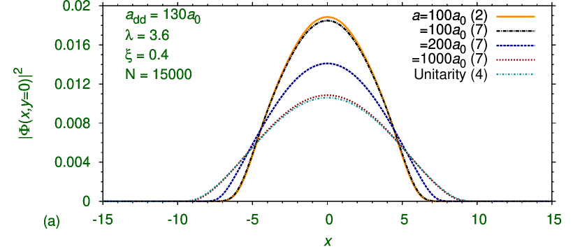
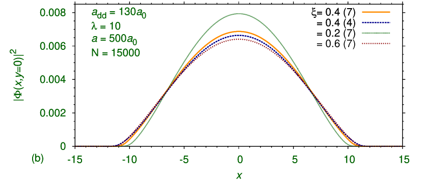
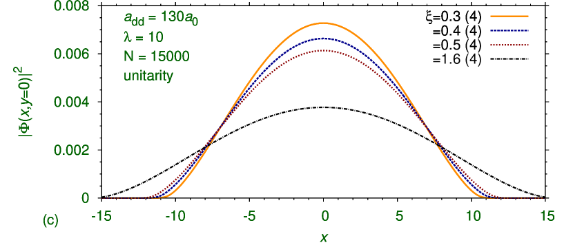
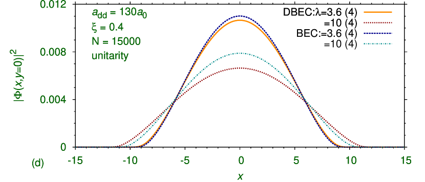
Figure 1: (Color online) (a) Radial density along $x$ axis $|\Phi(x,y=0)|^{2}=\int dz|\phi(x,y=0,z)|^{2}$ of a ¹⁶⁴Dy BEC with $N=15000$, $\lambda=3.6$, $a_{dd}=130a_{0},\nu=1$ and $\xi=0.4$ for $a=100a_{0},200a_{0},1000a_{0}$ and at unitarity using the GP limit (2), crossover model (7), and at unitarity (4). (b) The same for $\lambda=10$, $a=500a_{0}$ and $\xi=0.2,0.4,0.6$ using the crossover model (7). The density at unitarity (4) for $\xi=0.4$ is also shown. (c) The same for $\lambda=10$ and different $\xi$ at unitarity (4). (d) The same for $\xi=0.4,\lambda=3.6,10$ at unitarity (4) for $a_{dd}=130a_{0}$ (DBEC), and $a_{dd}=0$ (BEC).

In Fig. 1 (a), we plot the radial density of the BEC along $x$ axis $|\Phi(x,y=0)|^{2}$ obtained by integrating out the $z$ dependence of density: $|\Phi(x,y)|^{2}=\int dz|\phi(x,y,z)|^{2}$. In this figure we show the result for $a=100a_{0}$ using the GP model (2) and at unitarity (4) in addition to the results for $a=100a_{0},300a_{0},$ and $500a_{0}$ using the BEC-unitarity crossover model (7) with $\xi=0.4$ and $\nu=1$. For small $a$, the density from the crossover model (7) is in agreement with the GP model (2) and hence practically independent of the parameter $\xi$, whereas for large $a$ it approximates the unitarity limit (4) with the increase of $a$. In Fig. 1 (b) we plot the radial density for $a=500a_{0}$ for different $\xi$ using the crossover model (7). The result at unitarity (4) for $\xi=0.4$ is also shown. The density is sensitive to the parameter $\xi$ for $a=500a_{0}$ as can be seen from Fig. 1 (b) comparing the results for $\xi=0.2,0.4$ and 0.6. The sensitivity of the density on $\xi$ at unitarity is illustrated in Fig. 1 (c), where we show the radial density for $\xi=0.3,0.4,0.5$ and 1.6. Finally, in Fig. 1 (d) we show the density at unitarity for nondipolar and dipolar BECs for two values of the trap asymmetry $\lambda=3.6$ and 10. The difference between the two densities is more pronounced for $\lambda=10$, where the dipolar repulsion is stronger.

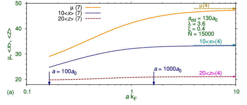
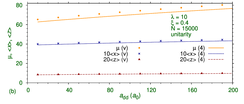
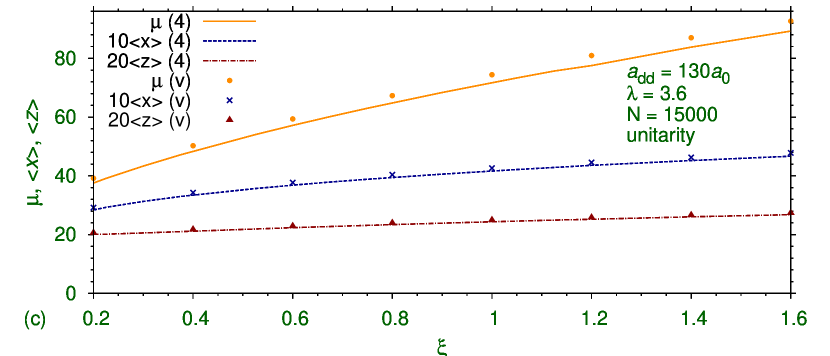
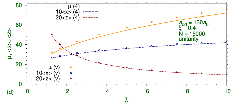
Figure 2: (Color online) (a) The numerical rms sizes $\langle x\rangle$, $\langle z\rangle$, and chemical potential $\mu$ of the dipolar BEC with $N=15000,a_{dd}=130a_{0},\xi=0.4,\nu=1,\lambda=3.6$ versus $ak_{F}$ using the crossover model (7), as well as at unitarity (4) (arrow). (b) The numerical (4) and variational (v) results for the same at unitarity versus $a_{dd}$. (c) The numerical (4) and variational (v) results for the same at unitarity versus $\xi$. (d) The numerical (4) and variational (v) results for the same at unitarity versus $\lambda$.

In Fig. 2 (a) we plot the rms sizes of the BEC $\langle x\rangle$, $\langle z\rangle$, and the chemical potential $\mu$ for $\xi=0.4,$ and $a_{dd}=130a_{0}$ as calculated using crossover model (7), versus the dimensionless parameter $k_{F}a$, where $k_{F}$ is the Fermi wave vector in a harmonic trap defined by $k_{F}=(48N)^{1/6}/\bar{l}$ rmp , where $\bar{l}=\sqrt{\hbar/m\bar{\omega}},\bar{\omega}=2\pi(f_{x}f_{y}f_{z})^{1/3}$, $\{f_{x},f_{y},f_{z}\}=\{436,436,1570\}$ Hz. One can find from Fig. 2 (a) how these quantities $-$ $\langle x\rangle$, $\langle z\rangle$, $\mu$ $-$ approach their values at unitarity as $a$ increases. With the increase of $a$ these quantities saturate rapidly to their respective values at unitarity. In Fig. 2 (b), we plot the numerical (n) and variational (v) results for $\langle x\rangle$, $\langle z\rangle$, and $\mu$ versus $a_{dd}$ at unitarity, which shows that the results are weakly sensitive to a variation of $a_{dd}$. In Fig. 2 (c) we plot $\langle x\rangle$, $\langle z\rangle$, and $\mu$ versus $\xi$ at unitarity, which shows that the results are sensitive to a variation of $\xi$. Finally, in Fig. 2 (d) we plot $\langle x\rangle$, $\langle z\rangle$, and $\mu$ versus $\lambda$ at unitarity showing the strong sensitivity of the results to a variation of $\lambda$. From Figs. 2 (b), (c), (d) we see that the variational results are in good agreement with the numerical ones.

In a recent experiment, Navon et al. bosuni1 were able to make measurements for densities of a very dilute BEC of ⁷Li for $a=2150a_{0}$ and extract the parameter $\xi$ from a theoretical analysis using the LHY correction lhy ; fp . The very dilute BEC prepared in a weak trap, allowed to make an experiment for large $a=2150a_{0}$. But because of the low density, the BEC remained away from the strong-coupling regime even for $a=2150a_{0}$ and was studied by the LHY correction, rather than a full crossover model as in the present study. In this regime the densities are weakly sensitive to the parameter $\xi$ and only an upper limit $\xi<0.6$ could be obtained from that study bosuni1 .

Apart from density profile and rms sizes of the dipolar BEC, other observables which can be studied are the frequencies of radial and axial oscillations $\Omega_{\rho}$ and $\Omega_{z}$, respectively, of the fundamental modes. We calculated these frequencies by numerically solving the variational equations (13a) and (13b) in different cases. The initial widths $w_{\rho}$ and $w_{z}$ were taken as their equilibrium static values and their time evolution is obtained. The frequencies of radial and axial oscillations were extracted from the time evolution of the respective widths. In Fig. 3 (a) we show these frequencies for $\xi=0.4$ versus $a_{dd}$ and in Fig. 3 (b) we plot these frequencies for $a_{dd}=130a_{0}$ versus $\xi$ for $\lambda=3.6,10$. We also calculated the axial frequency $\Omega_{z}$ from the small oscillation of the rms axial size of the BEC upon real time evolution of the mean-field equations (II.1) and (4). Because of a mixture of frequencies of higher modes, it was not possible to obtain precisely the frequency $\Omega_{\rho}$ from a solution of the mean-field equations. The mean-field and the variational results for $\Omega_{z}$ are in good agreement with each other. These frequencies are practically insensitive to a variation of $a_{dd}$ as well as of $\xi$. Hence it may not be very fruitful to study these frequencies in the strong-coupling regime in order to extract the parameter $\xi$, specially for a moderate density as in this study.

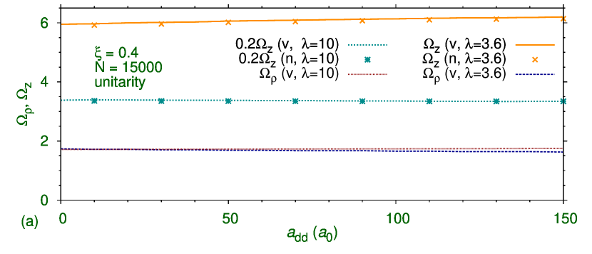
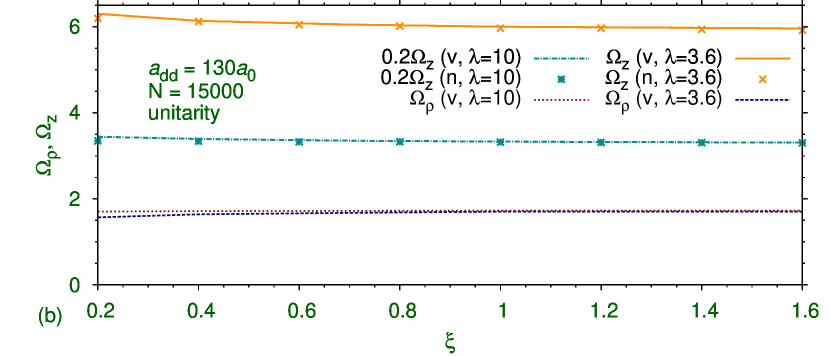
Figure 3: (Color online) (a) Variational frequency (v) of radial and axial oscillation $\Omega_{\rho}$ and $\Omega_{z}$ of the dipolar BEC with $N=15000,\xi=0.4,\nu=1,\lambda=3.6,10$ versus $a_{dd}$ at unitarity from Eqs. (13a) and (13b). The numerical frequencies (n) of axial oscillation obtained from a solution of Eqs. (II.1) and (7) are also shown. (b) The same for $a_{dd}=130a_{0}$ versus $\xi$.

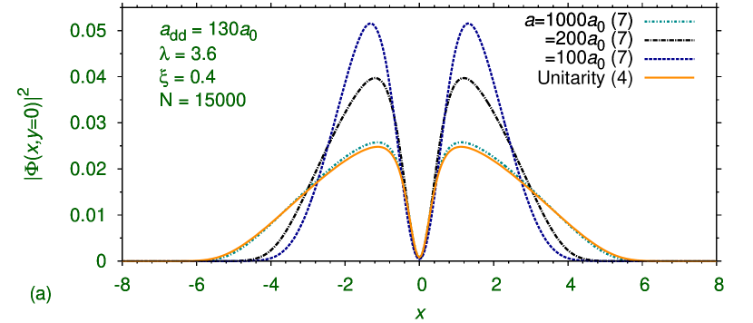
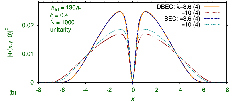
Figure 4: (Color online) (a) Radial density along $x$ axis $|\Phi(x,y=0)|^{2}$ of a ¹⁶⁴Dy BEC vortex of $N=1000$, $\lambda=3.6$, $a_{dd}=130a_{0},\nu=1$ and $\xi=0.4$ for $a=100a_{0},200a_{0},1000a_{0}$ and at unitarity using the crossover model (7), and at unitarity (4). (b) The same for $\xi=0.4,\lambda=3.6,10$ at unitarity (4) for $a_{dd}=130a_{0}$ (DBEC), and $a_{dd}=0$ (BEC).

III.3 Dipolar BEC Vortex

Next we study the density of a disk-shaped dipolar BEC vortex of unit angular momentum for strong-coupling and demonstrate the sensitivity of the result on the parameter $\xi$. In this case the radius of the vortex core is an observable directly related to the healing length rmp of the BEC and will also be considered. The radius of the vortex core $\rho_{c}$ is defined as the radial distance from the center of the vortex to a point where the density increases to the maximum value. It is more appropriate to consider the relative radius of vortex core defined by $r_{0}\equiv\rho_{c}/\langle x\rangle$, which gives the vortex core radius in relation to the radial size of the condensate. It is demonstrated that the relative vortex core radius $r_{0}$ could be sensitive to $\xi$ in the strong-coupling regime and could be useful in deciding the value of $\xi$.

In Fig. 4 (a), we plot the radial density of the BEC vortex along the $x$ axis $|\Phi(x,y=0)|^{2}$ for $N=1000$, $\lambda=3.6,a_{dd}=130a_{0},\xi=0.4,\nu=1$ for different values of scattering length $a$. In this figure we show the result for $a=100a_{0}$ and at unitarity (4) in addition to the results for $a=100a_{0},200a_{0},$ and $1000a_{0}$ using the BEC-unitarity crossover model (7). For small $a$, the density obtained using the crossover model (7) is in agreement with the GP equation (2) and hence independent of the parameter $\xi$, whereas for large $a$ it approximates the unitarity limit (4). In Fig. 4 (b), we show the radial density at unitarity for nondipolar and dipolar BECs for two values of the trap asymmetry $\lambda=3.6$ and 10. The difference between the two densities is more pronounced for $\lambda=10$, where the dipolar repulsion is stronger.

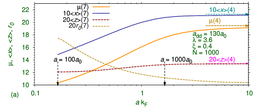
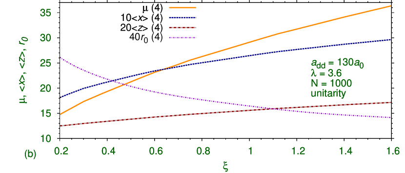
Figure 5: (Color online) (a) The rms sizes $\langle x\rangle$, $\langle z\rangle$, chemical potential $\mu$, and relative radius of vortex core $r_{0}$ of the dipolar BEC vortex with $N=1000,a_{dd}=130a_{0},\xi=0.4,\nu=1,\lambda=3.6$ versus $ak_{F}$ using the crossover model (7), as well as at unitarity (4) (arrow). (b) The same at unitarity (4) versus $\xi$.

In Fig. 5 (a) we plot chemical potential $\mu$ and rms sizes $\langle x\rangle$, $\langle z\rangle$ together with the relative radius of vortex core $r_{0}$ versus $ak_{F}$ for $N=1000,a_{dd}=130a_{0},\lambda=3.6,\xi=0.4,\nu=1$ obtained using the crossover model (7). The result at unitarity (4) is also shown. The relative radius of vortex core reduces with the increase of the scattering length. Similar reduction of the radius of vortex core was predicted for a nondipolar BEC before nilsen ; skab . In In Fig. 5 (b) we plot $\mu$,$\langle x\rangle$, $\langle z\rangle$, $r_{0}$ versus $\xi$ at unitarity (4) for $N=1000$, $\lambda=3.6,a_{dd}=130a_{0},\lambda=3.6,\nu=1$. As scattering length $a$ increases in Fig. 5 (a) or the parameter $\xi$ increases in Fig. 5 (b), the system becomes more repulsive leading to a smaller healing length. Consequently, the relative radius of vortex core $r_{0}$, which is closely related to the healing length, decreases rmp . The relative radius of vortex core shows much sensitivity to the scattering length $a$ and $\xi$.

IV Conclusion

The properties of a BEC at unitarity is controlled by a universal parameter $\xi$ relating the energies of noninteracting and unitary uniform gases. Using the BEC-unitarity crossover model (7) we studied the properties of a disk-shaped dipolar BEC and dipolar BEC vortex in the strong-coupling regime. We find that the density profiles are sensitive to the parameter $\xi$ in this regime and a study of density should yield an information about this parameter. We also studied the frequencies of the fundamental modes of radial and axial oscillation of this BEC and find that they are not much sensitive to $\xi$. For a dipolar BEC vortex, in addition to density, the relative radius of vortex core is also found to be sensitive to $\xi$ in the strong-coupling regime, so that a study of this radius may reveal information about $\xi$. Also to extract the parameter $\xi$ it is not necessary to study the system at unitarity. The density profile of the BEC is sensitive to the parameter $\xi$ for the contact interaction lying between the weak-coupling GP and strong-coupling unitarity limits, so that a study in this regime should reveal information about this parameter. In this study we used a dipolar BEC of 15000 ¹⁶⁴Dy atoms in a disk-shaped trap of anisotropy $\lambda=3.6$, as in the experiment of Ref. dy2 , and also $\lambda=10$. For an experimental study the anisotropy of $\lambda=10$, or larger, and a BEC with strong dipole interaction is to be preferred.

- (1) S. Giorgini, L. Pitaevskii, and S. Stringari, Rev. Mod. Phys. 80, 1215 (2008).
- (2) J. M. Diederix, T. C. F. van Heijst, and H. T. C. Stoof, Phys. Rev. A84, 033618 (2011).
- (3) G. E. Astrakharchik, J. Boronat, J. Casulleras, and S. Giorgini, Phys. Rev. Lett. 93, 200404 (2004).
- (4) J. Carlson and S. Reddy, Phys. Rev. Lett. 95, 060401 (2005); J. Carlson, S. Y. Chang, V. R. Pandharipande, and K. E. Schmidt, Phys. Rev. Lett. 91, 050401 (2003);
- (5) G. Partridge et al., Science 311, 503 (2006).
- (6) J. Kinast, A. Turlapov, and J. E. Thomas, Phys. Rev. Lett. 94, 170404 (2005).
- (7) M. Bartenstein et al., Phys. Rev. Lett. 92, 120401 (2004).
- (8) L. Luo and J. E. Thomas, J. Low Temp. Phys. 154, 1 (2009).
- (9) S. K. Adhikari, J. Phys. B 43, 085304 (2010).
- (10) N. Navon, S. Nascimbène, F. Chevy, and C. Salomon, Science 328, 729 (2010).
- (11) J. T. Stewart, J. P. Gaebler, C. A. Regal, and D. S. Jin, Phys. Rev. Lett. 97, 220406 (2006).
- (12) N. Navon et al., Phys. Rev. Lett. 107, 135301 (2011).
- (13) S. Cowell et al., Phys. Rev. Lett. 88, 210403 (2002).
- (14) J. L. Song and F. Zhou, Phys. Rev. Lett. 103, 025302 (2009).
- (15) Y.-L. Lee and Y.-W. Lee, Phys. Rev. A81, 063613 (2010).
- (16) S. K. Adhikari and L. Salasnich, Phys. Rev. A77, 033618 (2008).
- (17) S. Papp et al., Phys. Rev. Lett. 101, 135301 (2008).
- (18) S. E. Pollack et al., Phys. Rev. Lett. 102, 090402 (2009).
- (19) T. Koch, T. Lahaye, J. Metz, B. Frohlich, A. Griesmaier, and T. Pfau, Nature Phys. 4, 218 (2008).
- (20) T. Lahaye et al., Nature (London) 448, 672 (2007); T. Lahaye, C. Menotti, L. Santos, M. Lewenstein, and T. Pfau, Rep. Prog. Phys. 72, 126401 (2009).
- (21) M. Lu, S. H. Youn, and B. L. Lev, Phys. Rev. Lett. 104, 063001 (2010); J. J. McClelland and J. L. Hanssen, Phys. Rev. Lett. 96, 143005 (2006); S. H. Youn, M. W. Lu, U. Ray, and B. V. Lev, Phys. Rev. A82, 043425 (2010).
- (22) M. Lu, N. Q. Burdick, Seo Ho Youn, and B. L. Lev, Phys. Rev. Lett. 107, 190401 (2011).
- (23) S. Inouye et al., Nature 392, 151 (1998).
- (24) P. Muruganandam and S. K. Adhikari, Phys. Lett. A 376, 480 (2012); T. Lahaye et al. Phys. Rev. Lett. 101, 080401 (2008); C. Ticknor, R. M. Wilson, and J. L. Bohn, Phys. Rev. Lett. 106, 065301 (2011); C. Krumnow and A. Pelster, Phys. Rev. A84, 021608 (2011); I. Tikhonenkov, B. A. Malomed, and A. Vardi, Phys. Rev. Lett. 100, 090406 (2008); R. Nath, P. Pedri, and L. Santos, Phys. Rev. Lett. 102, 050401 (2009).
- (25) K. Góral and L. Santos, Phys. Rev. A 66, 023613 (2002).
- (26) S. Ronen, D. C. E. Bortolotti, and J. L. Bohn, Phys. Rev. Lett. 98, 030406 (2007); R. M. Wilson, S. Ronen, J. L. Bohn, and H. Pu, Phys. Rev. Lett. 100, 245302 (2008); M. Asad-uz-Zaman and D. Blume Phys. Rev. A 83, 033616 (2011); Phys. Rev. A 80, 053622 (2009); H. Saito, Y. Kawaguchi, and M. Ueda, Phys. Rev. Lett. 102, 230403 (2009).
- (27) M. Abad, M. Guilleumas, R. Mayol, M. Pi, and D. M. Jezek, Phys. Rev. A 81, 043619 (2010); O. Dutta and P. Meystre, Phys. Rev. A75, 053604 (2007); R. M. W. van Bijnen, A. J. Dow, D. H. J. O’Dell, N. G. Parker, and A. M. Martin, Phys. Rev. A 80, 033617 (2009); R. M. W. van Bijnen, N. G. Parker, S. J. J. M. F. Kokkelmans, A. M. Martin, and D. H. J. O’Dell, Phys. Rev. A 82, 033612 (2010); N. G. Parker, C. Ticknor, A. M. Martin, and D. H. J. O’Dell, Phys. Rev. A79, 013617 (2009); N. G. Parker and D. H. J. O’Dell, Phys. Rev. A 78, 041601 (2008); R. M. Wilson, S. Ronen, and J. L. Bohn, Phys. Rev. A80, 023614 (2009).
- (28) L. E. Young-S, P. Muruganandam, and S. K. adhikari, J. Phys. B 44, 101001 (2011); P. Muruganandam and S. K. adhikari, J. Phys. B 44, 121001 (2011); S. K. Adhikari and P. Muruganandam, J. Phys. B 45, in press (2012).
- (29) L. Santos, G. V. Shlyapnikov, P. Zoller, and M. Lewenstein, Phys. Rev. Lett. 85, 1791 (2000).
- (30) S. K. Adhikari and L. Salasnich, Phys. Rev. A78, 043616 (2008); S. K. Adhikari, H. Lu, and H. Pu, Phys. Rev. A 80, 063607 (2009).
- (31) T. D. Lee, K. Huang, and C. N. Yang, Phys. Rev. A106, 1135 (1957).
- (32) F. Dalfovo and S. Stringari, Phys. Rev. A 53, 2477 (1996).
- (33) A. Fabrocini and A. Polls, Phys. Rev. A64, 063610 (2001).
- (34) W. Lenz, Z. Phys. 56, 778 (1929).
- (35) D. Blume and C. H. Greene, Phys. Rev. A 63, 063601 (2001).
- (36) S. K. Adhikari, Phys. Rev. A70, 043617 (2004); S. K. Adhikari and B. A. Malomed, Europhys. Lett. 79, 50003 (2007).
- (37) V. M. Pérez-García, H. Michinel, J. I. Cirac, M. Lewenstein, and P. Zoller, Phys. Rev. A56, 1424 (1997).
- (38) S. Yi and L. You, Phys. Rev. A63, 053607 (2001); Phys. Rev. Lett. 92, 193201 (2004).
- (39) P. Muruganandam and S. K. Adhikari, Comput. Phys. Commun. 180, 1888 (2009).
- (40) A. Perali, P. Pieri, and G. C. Strinati, Phys. Rev. Lett. 93, 100404 (2004).
- (41) J. K. Nilsen et al., Phys. Rev. A71, 053610 (2005).