X-ray Emission Line Profiles from Wind Clump Bow Shocks in Massive Stars

Abstract

The consequences of structured flows continue to be a pressing topic in relating spectral data to physical processes occurring in massive star winds. In a preceding paper, our group reported on hydrodynamic simulations of hypersonic flow past a rigid spherical clump to explore the structure of bow shocks that can form around wind clumps. Here we report on profiles of emission lines that arise from such bow shock morphologies. To compute emission line profiles, we adopt a two component flow structure of wind and clumps using two “beta” velocity laws. While individual bow shocks tend to generate double horned emission line profiles, a group of bow shocks can lead to line profiles with a range of shapes with blueshifted peak emission that depends on the degree of X-ray photoabsorption by the interclump wind medium, the number of clump structures in the flow, and the radial distribution of the clumps. Using the two beta law prescription, the theoretical emission measure and temperature distribution throughout the wind can be derived. The emission measure tends to be power law, and the temperature distribution broad in terms of wind velocity. Although restricted to the case of adiabatic cooling, our models highlight the influence of bow shock effects for hot plasma temperature and emission measure distributions in stellar winds and their impact on X-ray line profile shapes. Previous models have focused on geometrical considerations of the clumps and their distribution in the wind. Our results represent the first time that the temperature distribution of wind clump structures are explicitly and self-consistently accounted in modeling X-ray line profile shapes for massive stars.

1 Introduction

The subject of X-ray production in massive star winds continues to be an evolving field of study. The superionization seen at UV wavelengths of OB stars were best explained by a model that had a source of X-rays in the winds (Cassinelli, Castor, & Lamers 1978; Cassinelli & Olson 1979). Initial observations by the Einstein observatory made the important discovery that essentially all O stars were X-ray sources (Harnden et al. 1979; Seward et al. 1979). A key finding to emerge from these early observations is that the observed X-ray luminosities are roughly correlated with the bolometric luminosities as $L_{X}\approx 10^{-7}L_{\rm Bol}$ (e.g., Cassinelli et al. 1981). Additional more extensive studies confirmed the relationship (e.g., Berghofer et al. 1997; Nazé et al. 2011), although the basis of the relationship continues to be a point of investigation (e.g., Owocki & Cohen, 1999; Owocki et al. 2011). In addition, the majority of OB stars display soft X-ray emissions with temperatures $kT<1$ keV (e.g., Berghofer et al. 1996; Güdel & Nazé 2009);

Two pictures for the X-ray emission from hot stars arose: one involving a coronal zone at the base of a cool wind (Cassinelli & Olson 1979) and one involving shocks that form by line-driven wind instabilities (Lucy & White 1980; Lucy 1982). The coronal model as the sole source of the observed X-ray emission was quickly ruled out based on analyses of the earliest higher spectral resolution observations using the Solid State Spectrometer (SSS) on the Einstein observatory. Cassinelli & Swank (1983) found that the predicted large X-ray optical depths expected for a base coronal source of X-rays were incompatible with the observed SSS spectra. They further suggested that these winds consist of many shock fragments to explain the lack of significant X-ray variability.

Studies of X-ray emissions from OB stars have focused primarily on exploring the wind driven instabilities (or line de-shadowing instability, LDI) as a process of producing a distribution of wind shocks (e.g., Owocki, Castor, & Rybicki 1988). A detailed picture of the expected X-ray production from these wind shocks was given by Feldmeier (1995), and Felmeier et al. (1997) showed that a wide range of temperatures could be produced in a planar shock front.

We are now in an era of high spectral resolution X-ray astronomy with a few dozen massive stars having been studied in long pointed observations (e.g., Walborn, Nichols, & Waldron 2009). Better quality data have led to a host of new questions concerning the physics of X-ray generation in massive star winds (e.g., Waldron & Cassinelli 2007; hereafter WC07). Most of the X-ray line emission is clearly formed within the winds. A triad of lines from He-like ions (forbidden, intercombination, and resonance or “fir” lines) provide direct information about the formation radius of X-ray line emission (Kahn et al. 2001; Waldron & Cassinelli 2001; Leutenegger et al. 2006). Supergiant winds typically show that the lower energy ion stages such as O vii tend to form near or above 10 $R_{\ast}$; intermediate energy ions (e.g., Ne ix and Mg xi) form deeper at $\approx 3$ to 8 $R_{\ast}$; and high energy ions such as Si xiii and S xv form relatively close to the star ($<2\hbox{$R_{\ast}$}$). Waldron & Cassinelli (2001) suggested that these differences in depths could perhaps be explained from considerations of wind absorption effects, since the cool wind opacity scales as $\kappa\propto\lambda^{3}$. Thus winds are more transparent at shorter wavelengths (higher energies). Waldron & Cassinelli (2001) also noticed that the location of line formation for the He-like ions appeared to correlate with the respective radii of optical depth unity for the X-ray photoabsorption (c.f., Cassinelli et al. 2001; Miller et al. 2002; Oskinova et al. 2006; WC07). The conclusion is that hot plasma is spatially distributed in the wind flow.

One surprising result from the high resolution X-ray spectroscopy data is the general symmetry of broad lines and the frequent absence of line profiles with significantly blue-shifted peak emissions. It had been expected that the wind X-ray lines would be generally broad yet skewed to the short wavelength (or “blueward”) side of the line. This skewness is a consequence the fact that for an expanding wind, the column depth of photoabsorption to the flow on the far side of the star is larger than on the near side, resulting in differential attenuation between the red and blueshifted hemispheres (MacFarlane et al. 1991; Ignace 2001; Owocki & Cohen 2001). So the observation of frequently symmetric and unshifted lines was unexpected for the massive winds of OB supergiants. For these stars WC07 found that $\approx 60\%$ of emission lines are broad with a mean line-width (HWHM) of 0.3 to 0.5 of the wind terminal speed ($V_{\infty}$), and in excess of 75% of the lines have line-shifts that lie within $\pm 0.2\hbox{$V_{\infty}$}$ of line center.

As suggested by Waldron & Cassinelli (2001), the simplest way to account for the rather symmetric and unshifted X-ray line profiles is that the wind is more optically thin to X-rays than suggested by the mass-loss rates. A variety of models have emerged to explain the line symmetry problem by studying wind clumping and wind porosity effects. Clumping in dense Wolf-Rayet winds has been known for many years (Moffat et al. 1988), and there is direct evidence of clumping among some O-stars (e.g., Lepine & Moffat 2008). Clumping can be categorized as ranging from micro-clumping (e.g., Hillier 1991; Hamann & Koesterke 1998) to macro-clumping (e.g., Feldmeier et al. 2003; Brown et al. 2004; Oskinova et al. 2004, 2006, 2007; Owocki & Cohen 2006), or a mix of the two. Micro-clumping explicitly assumes all clumps are optically thin at all wavelengths, which need not be the case for macro-clumping.

Reductions in the mass-loss rate $\dot{M}$ by a factor of 10 or more appeared to be supported by FUSE observations of Pv lines from several hot-stars (Fullerton et al. 2006). Although this would certainly make the winds more thin to X-rays, this severe reduction in $\dot{M}$ can be eliminated either by accounting for wind “macro-clumping” (Oskinova et al. 2007) or by including the effects of XUV radiation in reducing the fractional abundance of Pv (Waldron & Cassinelli 2010).

Other models that have been proposed to explain the symmetry of the X-ray lines include the effects of resonance line scattering on line shapes (Ignace & Gayley 2002), and there is support in one case where such effects are applicable (Leutenegger et al. 2007); two-component wind structures where the polar wind component is impeded by surface magnetic structures (Mullan & Waldron 2006); and models requiring magnetic fields and collisionless shocks (Pollock 2007).

Resolved X-ray lines have served as an impetus to understand more accurately the nature of the hot plasma component. And encoded within these detailed X-ray emission line shapes is the required information both about the formation process of the line (i.e., the density and temperature which determines the emissivity) and the vector velocity field. Although these various approaches have certainly had successes in trying to decode these line profiles, there remain open questions about understanding the temperature and emission measure distributions, and the radial location of hot plasma formation and maintenance. In particular, previous considerations of line profiles from clumpy/porous winds (e.g., Owocki & Cohen 2006; Oskinova et al. 2007) have focused on issues of clump geometry (pertaining to photon escape) and clump distributions (pertaining volume filling factors), but these have not self-consistently included temperature distributions implied by the structures themselves, as for example in planar shocks. Even smooth wind considerations have been geometrical in nature (e.g., Owocki & Cohen 2001; Ignace & Gayley 2002). The models presented here have the benefit of self-consistently including the detailed temperature distribution of the shocked structures, within the context of the assumed model.

The underlying model for clump bow shock structure was presented in Cassinelli et al. (2008; hereafter Paper I), who considered the shape, temperature, and density of bow shocks that form around wind clumps. In this second paper of the series, we are explicitly interested in the line profiles that form from these bow shock structures and how features of the clump bow shock paradigm may contribute to understanding the observed shapes of massive star X-ray line profiles. In section 2 the results of Paper I are briefly reviewed. In section 3, line profiles are calculated and discussed for individual clump bow shocks, emphasizing the diversity of line shapes that can result. Section 4 describes line profiles that from an ensemble of clumps, including the limitng case of many clumps and the case of a discrete ensemble of randomly placed clumps. Section 5 presents concluding remarks about these results and needed future areas of stdy. The Appendix details considerations of the temperature distribution in the wind for our model prescription.

2 Model Description

Our model calculations of X-ray emission line profiles produced by a wind distribution of clumps and their associated bow shock structures are based on simulations discussed in Paper I. Our results apply to the hypersonic limit, namely that the Mach number is high ( $\gtrsim~{}10$), which is an excellent description of the situation in a massive star wind where the terminal speed $\hbox{$V_{\infty}$}\sim 1000$ km s^-1 and the gas thermal speed is $\approx 100$ times smaller. This means that the bow shock structure – its shape, and its relative density and temperature distributions – are largely independent of the actual Mach number (e.g., Hayes & Probstein 2004).

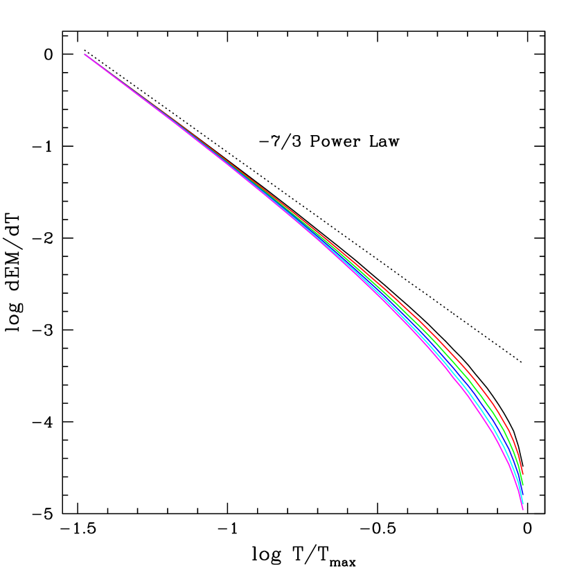
Figure 4: A logarithmic plot of the intrinsic total DEM against temperature in the smooth wind limit. Temperature is normalized to $T_{\rm max}$. Curves are for $\beta_{\rm cl}$ values of even integers between 2 to 12, inclusive. The dotted line is for a $-7/3$ power law as would apply to a single clump. The curves have been shifted to have the same value at the lowest temperature for ease of comparison. Despite the wide range of $\beta_{\rm cl}$ values, similar overall DEM distributions result.

However, since line profile calculations require detailed information on the actual velocity field of a large number of wind distributed clumps, we need to establish the distribution of the line-of-sight (LOS) velocities as seen by an observer. The simulations of Paper I were carried out in the rest frame of a rigid and spherically symmetric clump where a fast moving wind with plane parallel symmetry and constant density sweeps across the face of a clump. The plane-parallel approximation applies when the the radius of the clump, $R_{\rm cl}$, is small compared to the wind clump radial location, $r$. To compute synthetic line profile shapes the vector velocity field for the bow shock found in Paper I (see their Fig. 4), which is accomplished through relative velocity vector defined by

$${\bf\Delta V(r)}=\left[V_{W}(r)-V_{\rm cl}(r)\right]\,{\bf\hat{r}}$$ (1)

where $V_{W}$ is now the preshock ambient (or inter-clump) stellar wind speed at the site of the clump, $V_{\rm cl}$ is the clump speed, and both are measured relative to the stellar rest frame. We are assuming that $V_{W}$ and $V_{\rm cl}$ are purely radial and thus functions only of $r$. Note that the magnitude $\Delta V$ is the same in both the stellar and clump rest frames.

Our calculations apply to both cases of a clump moving faster or slower than the ambient medium because the simulations are conducted in the rest frame of the clump. As long as the relative velocity ($\Delta V$) between the clump and the surrounding gas medium is hypersonic, the same bow shock structure results. The only practical difference for line profiles is in which direction the bow shock opens with respect to the star center. If the clump is moving radially outward faster than the wind, the stagnation point will be ahead of the clump, and the bow shock opens toward the star. Similar scenarios have been discussed by Guo (2010) and Waldron & Cassinelli (2009). If the clump is slow, then the geometry flips by $180^{\circ}$, like in the application to $\tau$ Sco for infalling clumps (Howk et al. 2000).

An evaluation of the line profile shape requires knowledge of the LOS Doppler shifts toward an observer in a specified direction. Evaluating the Doppler shifts requires the introduction of several coordinate systems. We assume that the stellar wind is structured but spherical in a time averaged sense. With no special direction, the stellar and observer coordinate systems are chosen to be conincident. Cartesian coordinates $(X,Y,Z)$ are introduced, with associated standard spherical coordinates $(r,\vartheta,\varphi)$, where the polar angle $\vartheta$ is measured from the $+Z$ axis. The observer is located along the $+Z$ axis.

For each clump we adopt the cylindrical coordinate system $(\varpi,\phi,z)$ used in Paper I, where the $z$-axis in cylindrical coordinates coincides with the symmetry axis of the bowshock, and $\varpi$ is the cylindrical radius. The clump center corresponds to $\varpi=0$ and $z=0$.

In addition, since we envision these clumps as moving radially from the star, the symmetry axis of the bow shock is also the radial line from the star center to the clump center. Hence, a key condition inherent in these two coordinate system definitions is that ${\bf\hat{z}\cdot\hat{r}}=\pm 1$ is maintained for all wind distributed clumps, where the sign indicates whether the bow shock opens away from the star ($+$) or toward the star ($-$).

The specific points of our model are discussed in the following sections. We first start with a brief review of the bow shock properties found in Paper I as modified by using a relative velocity.

2.1 Overview of the Bow Shock Properties

2.1.1 Geometry

The numerical simulations of Paper I showed that the shape of the bow shock can be well-described by the form

$$\frac{z-z_{0}}{R_{\rm cl}}=a\left(\frac{\varpi}{R_{\rm cl}}\right)^{m},$$ (2)

with $a=0.35$, $m=2.34$, and $z_{0}=-1.19R_{\rm cl}$, hence a shape not far from a parabola. The bow shock apex forms at a distance of $0.19R_{\rm cl}$ above the clump surface.

In addition to the bow shock shape, it was demonstrated that the derivative of the bow shock shape (i.e., the position-dependent tangent) is the key parameter in determining the velocity, temperature $T$, and emission measure $EM$ distributions along the bow shock surface. In Paper I we defined this derivative as

$$\frac{dz}{d\varpi}\equiv g(\varpi)=a\,m\,(\varpi/R_{\rm cl})^{m-1},$$ (3)

It is convenient here to introduce an angle $\alpha$ that is related to the curvature of the bow shock, with

$$\tan\alpha=g(\varpi).$$ (4)

Note that in Paper I, we had defined this angle as $A_{1}$ but here prefer to use $\alpha$.

2.1.2 The Velocity Field

One of the major findings from Paper I was that the $EM$ was dominated by the immediate post-shock gas. So an “On The Shock” (OTSh) approximation was introduced, whereby the density $N$, temperature, and velocity relevant to X-ray observables are described by conditions along the bow shock surface, and thus by the geometry described in the preceding section. Hence, the velocity field in the rest frame of the clump that is needed to synthesize line profiles is known analytically at every point along the bow shock for the known surface geometry.

The simulation was based on the assumption that the radius of the clump $R_{\rm cl}\ll r$, so that the incident interclump wind flow was essentially plane parallel. Thus ${\bf\Delta V}=\Delta V\,\hat{z}$ in the rest frame of a clump itself (c.f., Fig. 4 of Paper I). We introduce the unit vectors $\hat{n}$ as the outward normal to the shock and $\hat{l}$ as a unit vector parallel to the shock in the direction away from the apex. The jump conditions for a strong oblique shock were applied to derive the velocity components perpendicular and parallel to the shock front. Using primes to denote velocities in the clump rest frame, the post-shock velocity components are given by

$${\bf V^{\prime}}_{P,\perp} = -\frac{1}{4}\,|\Delta V|\,\cos\alpha\,\hat{n}$$

$$= -\frac{1}{4}\,\frac{1}{\sqrt{1+g^{2}}}\,|\Delta V|\,\hat{n},$$

$${\bf V^{\prime}}_{P,\parallel} = |\Delta V|\,\sin\alpha\,\hat{l}$$

$$= \frac{g}{\sqrt{1+g^{2}}}\,|\Delta V|\,\hat{l}$$

where $\Delta V$ is from equation (1). Note that $\Delta V$ can be positive or negative depending on whether the clump is traveling faster or slower than the interclump wind, but the perpendicular velocity component is always away from the bow shock symmetry axis, and the parallel component is always downwind of the apex position.

The postshock velocity field is a function of clump’s radial distance from the star via $\Delta V$ and also location along the bow shock implicitly through the curvature factor $g(\varpi)$. The total postshock flow speed anywhere along the bow shock is

$$V^{\prime}_{P}=\frac{1}{4}\,\sqrt{\frac{1+16g^{2}}{1+g^{2}}}\,\Delta V.$$ (7)

As expected, the postshock velocity takes on a value of $V^{\prime}_{P}=\Delta V/4$ for a head-on collision at the bow shock apex where $g=0$. Far downstream of the apex, the speed approaches $V^{\prime}_{P}=\Delta V$ for $g\gg 1$ as the shock becomes extremely oblique.

In order to determine Doppler shifts of the X-ray emitting material, the postshock velocity field must be evaluated in the observer frame. To accomplish this, it is convenient to express the vector flow in the clump system as components of $\hat{z}$ and $\hat{\varpi}$ which can readily be transformed to the star/observer system. This requires a standard rotation of coordinate systems from $\hat{n}$ and $\hat{l}$ to $\hat{\varpi}$ and $\hat{z}$, which is given by

$$\hat{n} = \hat{\varpi}\sin\alpha\mp\hat{z}\cos\alpha$$

$$\hat{l} = \hat{\varpi}\cos\alpha\pm\hat{z}\sin\alpha$$

The distinction in sign for the $z$-component is related to whether the clump moves faster or slower than the interclump wind. If slower, then the bow shock opens away from the star and the upper sign is used; if faster, then the bow shock opens toward the star, and the lower sign is used.

With these preceding expressions, the postshock velocity in the rest frame of the star (unprimed system) becomes

$${\bf V}_{P} = {\bf V}^{\prime}_{P}+V_{\rm cl}\,\hat{z}$$ (8)

$$= |\Delta V|\,\left[\frac{3}{8}\sin 2\alpha\,\hat{\varpi}\pm\frac{1}{4}(1+3\sin^{2}\alpha)\,\hat{z}\right]$$

$$+V_{\rm cl}\,\hat{z},$$

$$\equiv V_{\varpi}\,\hat{\varpi}+\left[V_{\rm cl}+V_{\rm z}\right]\,\hat{z},$$ (9)

where $V_{\varpi}\geq 0$ is always true, but $V_{\rm z}\geq 0$ for the case that the clumps are slower than the interclump wind and $V_{\rm z}\leq 0$ for clumps that are faster.

The observed velocity shift for flow at a point in the wind is $v_{Z}=-\hat{Z}\cdot{\boldmath V}_{P}$, using lowercase “$v$” to signify that the velocity is for the observer. Carrying out the dot product yields

$$v_{Z}=-\left[V_{\rm cl}+V_{\rm z}\right]\,\cos\vartheta+V_{\varpi}\,\cos\varphi\,\sin\vartheta.$$ (10)

Owing to axial symmetry of the bow shock, $V_{\varpi}$ and $V_{\rm z}$ are functions only of distance from the bow shock apex along its surface. The velocity field reduces to $V_{P}\approx V_{\varpi}$ near the bow shock apex and $V_{P}\approx V_{\rm z}$ in the far outer wings of the bow shock.

2.1.3 The Temperature and Emission Measure Distributions

With the OTSh approximation, the runs of $T$ and $EM$ along the shock are monotonic functions of path length from the shock stagnation point. The peak temperature at the bow shock apex of an individual clump is $T_{A}$ with a value given by

$$T_{A} = \frac{3}{16}~{}\frac{\mu m_{H}}{k}~{}\Delta V^{2}$$ (11)

$$= 14~{}\mbox{MK}\,\left(\frac{\mu}{0.62}\right)\,\left(\frac{\Delta V}{1000~{}\hbox{km$\,$s${}^{-1}$}}\right)^{2},$$ (12)

where in the latter expression we have evaluated the constants assuming a fully ionized gas with solar abundances.

The path length downwind of the apex can be expressed as a function of impact parameter $\varpi$ for known bow shock geometry $z(\varpi)$. The postshock temperature, $T$, along the shock is found to be

$$T(\varpi)=\left(\frac{1}{1+g^{2}}\right)~{}T_{A}.$$ (13)

The power-law form of equation (3) provides $g(\varpi)$, and the temperature distribution reduces to

$$\frac{T}{T_{A}}=(1~{}+~{}g^{2})^{-1}=\left[~{}1~{}+~{}0.67\left(\frac{\varpi}{R_{\rm cl}}\right)^{2.68}\right]^{-1}$$ (14)

The line profile calculation also requires an emission measure distribution. A result of Paper I was that the differential emission measure ($DEM=dEM/dT$) is a monotonic power-law function of temperature and thus location along the bow shock with distance from the apex. One can conveniently parameterize the distribution with

$$\frac{dEM}{dT}=\frac{EM_{\circ}(r)}{T_{A}(r)}\,\left(\frac{T}{T_{A}}\right)^{-7/3}.$$ (15)

where the mapping between $\varpi$ and $T$ is made through the factor $g$ using equation (14). The emission measure scaling parameter $EM_{\circ}$ is given by

$$EM_{\circ}=5.1\times 10^{51}~{}{\rm cm}^{-3}\,\left(\frac{R_{\rm cl}}{10^{10}}\right)^{3}\left(\frac{N_{W}}{10^{10}}\right)^{2}\left(\frac{\hbox{$\Delta\ell$}}{R_{\rm cl}}\right),$$ (16)

where we have assumed a strong shock such that the postshock number density is $N_{P}=4N_{W}$, where $N_{W}$ is the preshock interclump wind number density, and $R_{\rm cl}$ and $N_{W}$ have both been scaled to the values used in the simulation. From Paper I, we found that $\hbox{$\Delta\ell$}=0.1R_{\rm cl}$ well approximates the simulation results. Our model does not predict the evolution of $R_{\rm cl}$ through the flow. To compare most easily our results with those of previous works, we adopt a scaling of $R_{\rm cl}^{3}\propto r^{2}$. Implicit then is that the emission measure varies as $EM_{\circ}\propto(rV_{W})^{-2}$ in form, like a smooth wind with a constant filling factor of hot plasma (e.g., Ignace 2001).

2.1.4 The Interclump and Clump Velocity Distributions

The critical parameter of the bow shock model is the relative velocity defined in equation (1) since it determines the magnitude of both the postshock X-ray temperature structure and the velocity field. Our approach is to assume a two-component wind model where the ambient wind and clump entities follow different velocity laws. We adopt the commonly used standard $\beta$ velocity law prescription defined as

$$V(r)=V_{\infty}\,\left(1-\frac{b}{r}\right)^{\beta},$$ (17)

with $V_{\infty}$ the terminal speed and $b<R_{\ast}$ so that the radial wind speed is non-zero at the wind base taken to be the stellar radius $R_{\ast}$. The value of $b$ sets the initial flow speed $V_{0}$, with

$$V_{0}=V_{\infty}\,\left(1-\frac{b}{R_{\ast}}\right)^{\beta}.$$ (18)

In all cases considered, the $b$ parameter will be fixed at the same value in both the interclump and clumped wind velocity laws. In order to limit the number of free parameters for our exploratory investigation, we also assume that both components achieve the same terminal speed.

The smooth interclump wind component will be described by the parameter $\beta_{W}$. Throughout this paper, we adopt $\beta_{W}=1$ as typical of OB star wind solutions. Then $\beta_{\rm cl}$ represents possible clump velocity distributions. Note that $\beta_{\rm cl}>\beta_{W}$ implies slow moving clumps relative to the interclump flow; $\beta_{\rm cl}<\beta_{W}$ corresponds to fast moving clumps.

2.2 Scalings from the $\beta$-Law Prescription

The distributions of $T_{\rm A}$ and the $DEM$ can be derived from the two $\beta$ approach. We introduce the convenient velocity normalization $w=V_{W}/V_{\infty}$. With the terminal speeds for the clump and interclump flows the same, the relation between the two components’ velocity laws are $w=w_{\rm cl}^{\beta_{\rm cl}}$, where $w_{\rm cl}=V_{\rm cl}/V_{\infty}$. Thus the velocity jump of equation (1) becomes

$$\Delta V=V_{\infty}\,w\,\left[1-w^{(\beta_{\rm cl}-1)}\right].$$ (19)

This relation can be used to find $T_{A}(r)$, which proceeds as follows.

Equation (12) along with the preceding expression gives

$$T_{A} = \frac{3}{16}~{}\frac{\mu m_{H}}{k}~{}\Delta V^{2},$$ (20)

$$= \frac{3}{16}~{}\frac{\mu m_{H}}{k}~{}V_{\infty}^{2}\,\left\{w\,\left[1-w^{(\beta_{\rm cl}-1)}\right]\right\}^{2},$$ (21)

$$\equiv T_{\rm lim}\,\left\{w^{2}\,\left[1-w^{(\beta_{\rm cl}-1)}\right]^{2}\right\},$$ (22)

where $T_{\rm lim}$ is implicitly defined as the highest possible temperature in our model of outflow that occurs for a velocity jump that is equal to the wind terminal speed.

Now the maximum hot plasma temperature $T_{\rm max}$ in the wind model can be determined. In the velocity coordinate of the interclump flow, $T_{\rm max}$ is achieved at a critical value $w_{\rm c}$ as given by

$$w_{\rm c}=\left(\frac{1}{\beta_{\rm cl}}\right)^{1/(\beta_{\rm cl}-1)},$$ (23)

which in the clump velocity becomes

$$w_{\rm cl,c}=\left(\frac{1}{\beta_{\rm cl}}\right)^{\beta_{\rm cl}/(\beta_{\rm cl}-1)}.$$ (24)

The radial location of $T_{\rm max}$ is at a corresponding critical radius value of $r_{\rm c}$, with

$$r_{\rm c}=\frac{b}{1-w_{\rm c}}.$$ (25)

The value of $T_{\rm max}$ is determined by just two parameters: the value of $\beta_{\rm cl}$ and the wind terminal speed via $T_{\rm lim}$, as given by

$$T_{\rm max}=T_{\rm lin}\,\left(\beta_{\rm cl}-1\right)^{2}\,\beta_{\rm cl}^{-2\beta_{\rm cl}/(\beta_{\rm cl}-1)}.$$ (26)

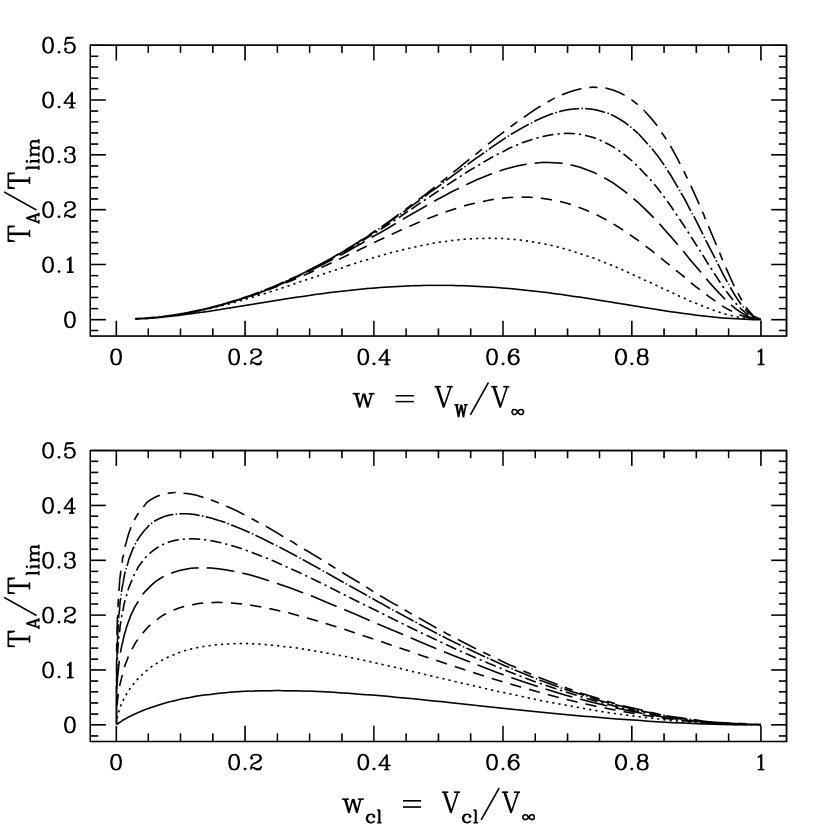
Figure 1: A plot of bow shock apex temperatures $T_{A}$ for clumps located at different positions in the wind. The temperature is normalized to $T_{\rm lim}$ (see text). The upper panel shows location in terms of the interclump wind velocity; lower is for the clump velocity. Curves are for different $\beta_{\rm cl}$ values, ranging from 2 (lowest curve) to 8 (highest curve) in integer intervals.

Figure 1 shows the distribution of $T_{A}$ in terms of the maximum possible temperature $T_{\rm lim}$ with different curves for different values of $\beta_{\rm cl}$. This is plotted against the normalized velocity of the interclump wind in the upper panel, and against the normalized velocity of the clumps in the lower panel. The curves range from $\beta_{\rm cl}=2$ (lowest curve) to $\beta_{\rm cl}=8$ (highest curve) in integer values. As $\beta_{\rm cl}$ increases, $T_{\rm max}$ shifts to progressively higher velocities of the interclump wind but lower velocities for the clump flow. Values of $T_{A}$ at different velocity locations are at the level of a tenth to a few tenths of $T_{\rm lim}$. For typical massive star wind speeds of 1000–3000 km s^-1, $T_{\rm lim}$ has values of 10–100 MK.

3 Line Profiles for An Individual Clump

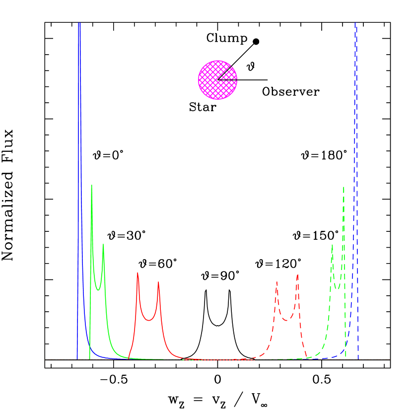
Figure 2: The inset (top center) shows the location of a clump at angle $\vartheta$ around the star from the observer’s axis. The plot shows example emission line profiles, all normalized to have unit area, for individual clumps located at the indicated orientations. In each case the clump is at the same radius, and so all profiles have the same apex temperature $T_{A}$. Solid curves are for clumps on the nearside of the star; dashed are for ones on the far side.

Before developing emission line profiles for clumped winds, it is instructive first to consider the emission line shape arising from a single clump. As an example case, we consider a clump at a location of $2R_{\ast}$ that follows a $\beta_{\rm cl}=3$ velocity law. The velocity jump is $\Delta V\approx 0.4V_{\infty}$. Figure 2 demonstrates the diversity in profile shapes for this single clump when it is located at different positions around the star, as given by the angle $\vartheta$ illustrated by the inset. The abscissa is the LOS observer velocity shift $w_{Z}=v_{Z}/V_{\infty}$. Note that the profiles have been normalized to have unit area. Values of $\vartheta=0^{\circ},30^{\circ},60^{\circ},90^{\circ},120^{\circ},150^{\circ},$ and $180^{\circ}$ were considered as labeled. For this figure both stellar occultation and absorption of X-rays by the clump itself are ignored, and the interclump wind is taken to be completely optically thin to X-rays.

Except for $\vartheta=0^{\circ}$ and $180^{\circ}$ which are clumps that lie along the LOS to the star, the profiles tend to be double-peaked and asymmetric. One exception is when a clump is at $\vartheta=90^{\circ}$; the profile is still double peaked but also symmetric since it lies in the plane of the sky with the star center. Generally, the double-horn shape is a consequence of the complex velocity field in the bow shock. The shapes become more nearly single-peaked as they approach the LOS to the star center. This is because the observer views the bow shock exactly along its symmetry axis. In conclusion, for a clump at $\vartheta=0^{\circ}$ and $180^{\circ}$, only the $V_{\rm z}$ component contributes to observed Doppler shifts, but for a clump located at $\vartheta=90^{\circ}$, only the $V_{\varpi}$ component contributes.

For the profiles of Figure 2, emission from the bow shock contributes from the peak temperature $T_{\rm A}$ down to an imposed minimum of 0.5 MK, which we use as a low temperature cut-off for hot plasma X-ray production. However, real lines form only over a restricted temperature range with consequences for the line shape. Consider a hypothetical line that forms between 2 and 3 MK. For a bow shock with $\hbox{$T_{\rm A}$}=10$ MK, this line would arise spatially from an annular band centered on the symmetry axis of the bow shock and offset from its apex. Consequently, realistic lines that form over different temperature ranges will tend to have different shapes, because they sample different portions of the postshock velocity field.

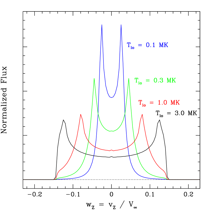
Figure 3: Similar to Fig. 2 but now profiles are for clumps only at $\vartheta=90^{\circ}$ and with different temperature intervals. The emissivity is taken to be constant within the temperature range of $T_{\rm lo}$ up to $T_{A}$, with $T_{\rm lo}=0.1,0.3,1.0,$ and 3.0 MK from the most narrow line (blue) to the broadest one (black), respectively.

Figure 3 illustrates this effect through the use of simple temperature cut-offs. The different curves are for line emission with different low temperature thresholds $T_{\rm lo}$. Below $T_{\rm lo}$ the emissivity is zero; above it the emissivity is independent of $T$. In this example clumps are placed at $\vartheta=90^{\circ}$. The profiles becomes progressively broader as the lower temperature cut-off increases, with values of $T_{\rm lo}=0.1$ MK (blue), 0.3 MK (green), 1.0 MK (red), and 3.0 MK (black).

To understand the growing line width with increasing $T_{\rm lo}$, recall that the $EM$ of a clump is dominated by the low temperature gas. For a clump at $\vartheta=90^{\circ}$, the bow shock is viewed perpendicular to its symmetry axis. Only $V_{\varpi}$ components of the postshock velocity field contribute to observed Doppler shifts. With the lowest temperature gas found furthest downwind of the bow apex, where the velocity vector is more nearly tangent to our LOS, $V_{\varpi}$ tends to be relatively small. Lower speed flow in the bow shock is to be found closer to the apex; however, this flow has a relatively larger component in the $\hat{\varpi}$ direction because of the greater curvature, with higher LOS Doppler shifts resulting at the bowhead. But the bowhead is exactly where the hottest plasma is to be found. Thus raising $T_{\rm lo}$ means that the bowhead region increasingly dominates the line formation, typically leading to a broader line for the given geometry.

Two final comments. First since increasing $T_{\rm lo}$ restricts the contributing volume, higher values of $T_{\rm lo}$ also lead to weaker lines for a given clump. This is not apparent from Figure 3 because each profile is normalized to unit area. Second, the stagnation point at the bowhead is the hottest gas and has intrinsically very low speed flow in the clump rest frame. If $T_{\rm lo}$ were to approach the value of $T_{\rm A}$  the profiles would actually narrow, a limit not reached in the exampes of Figure 3.

4 Line Shapes from an Ensemble of Clumps

Although it is important to understand the emission profile from an individual clump bow shock, stellar winds are understood to be highly structured from many lines of evidence (e.g., Lupie & Nordsieck 1987; Hillier 1991; Mofatt & Robert 1994; Lepine & Moffat 1999, 2008; Oskinova, Feldmeier, & Hamann 2004; Owocki & Cohen 2006; Prinja & Massa 2010; Muijres et al. 2011). Within our framework, this means there is more than one clump. Foremost is the basic observation that X-ray emissions from single massive stars are not highly variable. Although there is suggestive evidence of line variability (e.g., Nichols et al. 2011; Hole & Ignace 2012), in terms of bandpass luminosities, OB stars are typically variable at the level of 10% or less (Cassinelli & Swank 1983; Berghoefer & Schmitt 1994; Berghoefer et al. 1996, 1997).

Since we know that the observed X-ray emission from these stars arises from a wind distribution of X-ray sources, we now need to consider an ensemble of clump bow shocks for producing synthetic line profiles. We recognize the intrinsic time-dependent nature of the problem which, in principle, requires a full radiation hydrodynamics approach (e.g., Dessart & Owocki 2003, 2005). Since a goal of this paper is to present an initial analysis of line shapes arising from bow shock structures, such a detailed approach beyond the scope of this paper. Our basic premise is that observed emission lines reflect a time averaged wind flow. High energy resolution X-ray spectroscopy of high signal-to-noise requires exposure times ranging from 50 to 200 ks. By contrast, the characteristic flow time in a massive star wind is $R_{\ast}/v_{\infty}\sim 1-10$ ks. This means that a typical massive star X-ray spectrum is formed over multiple flow times, which tends to average over structural variations that are stochastic.

4.1 The Limit of Many Clumps

Having considered emission profiles from an individual clump in section 3, here we consider the opposite extreme of many clumps, which we refer to as the effectively “smooth” limit. It is imagined that large numbers of clumps are uniformly distributed in radius and orientation about the star to achieve strict spherical symmetry. Certainly, approximate spherical symmetry is consistent with low limits on the net continuum polarizations in O stars (McDavid 2000; Clarke et al. 2002). Polarization of unresolved sources is related to deviations of a circumstellar envelope from spherical (e.g., Brown & McLean 1977; Brown, Ignace, & Cassinelli 2000).

The idealized smooth limit has value in establishing a reference baseline of models that can be used for interpreting line profiles from winds with different degrees of structuring and time varying effects. (The latter will be treated in a separate paper.) Additionaly, the smooth limit allows for a derivation of the DEM from the wind as a whole. We begin this process by referring to equation (15) that describes the DEM of a single clump. The parameters $EM_{\circ}$ and $T_{\rm A}$ are themselves functions of clump location via equations (12) and (16). Both of these are functions of radius (or equivalently velocity) alone. Consequently, every clump in a shell of radius $r$ will have exactly the same DEM. The global DEM for the wind will consist of integrating contributions provided by every shell.

Working in the velocity coordinate of the interclump wind $V_{W}$, the total wind DEM is given by

$$\left(\frac{dEM}{dT}\right)_{\rm tot}=\int_{V_{1}(T)}^{V_{2}(T)}\,\frac{dEM}{dT}\,\frac{dN}{dV_{W}}\,dV_{W},$$ (27)

where $dN/dV$ represents the clump distribution in terms of radial velocity. In the limiting case of many clumps uniformly distributed in velocity, $dN/dV$ is a constant. To find the total DEM, the integration proceeds only over shells where the temperature $T$ is high enough to produce X-ray emission.

As described previously, there is a maximum temperature located in the wind at radius $r_{\rm c}$ with corresponding normalized velocity $w_{\rm c}$. The description of apex temperatures is thus double valued with radius. Plus, any given shell will have a range of temperatures from $T_{\rm A}$ down to a lower cut-off value. Clearly, a particular value of $T$ will only be found in a shell if $\hbox{$T_{\rm A}$}(V_{W})>T$. It is this condition that is used in equation (27) for the limits of the integrand.

Using results from the preceding section and equations (12) and (16), equation (27) becomes

$$\left(\frac{dEM}{dT}\right)_{\rm tot} \propto \left(\frac{T}{T_{\rm lim}}\right)^{-7/3}\,\int_{w_{1}}^{w_{1}}\,\left(\frac{1-w}{w}\right)^{2}$$

$$\times\left\{w^{2}\,\left[1-w^{(\beta_{\rm cl}-1)})\right]\right\}\,\Gamma(w)\,dw,$$

where $w_{1}$ and $w_{2}$ represent the velocity interval between which $T$ is achieved, and $\Gamma$ is a correction factor for stellar occultation. The latter is given by

$$\Gamma=\frac{1}{2}\,\left[1+\sqrt{1-\left(\frac{1-w}{b}\right)^{2}}\right].$$ (29)

Note that the integral is over a fixed $T$, hence the temperature dependence $T^{-7/3}$ can be factored out of the integral. Thus the integral that remains represents a temperature-dependent modification to the power law for a single clump. The integrand is not overly complex, but the integration limits $w_{1}(T)$ and $w_{2}(T)$ tend not to be analytic. (See App. B for solutions of $w_{1}$ and $w_{2}$ in the special cases of $\beta_{\rm cl}=1/2,2$, and 3.)

Figure 4 displays the results of calculations for the total DEM of the wind at even values of $\beta_{\rm cl}$ from 2 to 12. The DEM is plotted logarithmically against $T/T_{\rm max}$. The curves have been shifted to a zero value at the lowest temperature used. The results all lie very close to each other with departures from a $-7/3$ slope occuring only at higher values of $T$, as emphasized by the dotted line for a power-law of $-7/3$ slope. Different $\beta_{\rm cl}$ values yield the $-7/3$ slope at low $T$ because in our model the cooler X-ray emitting plasma is to be found essentially throughout the wind. The slight steepening toward larger $T$ becomes a downturn as $T_{\rm max}$ is approached, because only the hottest components are severely restricted in radial locale.

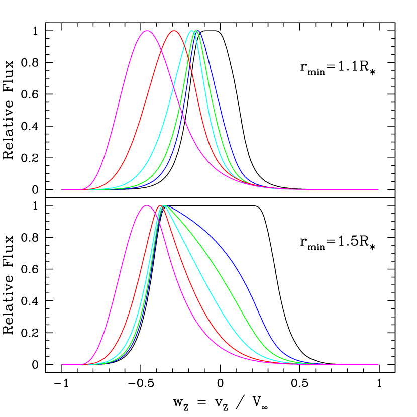
Figure 5: Illustrative emission line profiles for the smooth limiting case. Hot plasma is assumed not to exist interior to $r_{\rm min}$, with a value of $1.1R_{\ast}$ for the upper panel and $1.5R_{\ast}$ for the lower one. These models are for fast clumps with $\beta_{\rm cl}=0.5$. Different colored curves are for different levels of interclump wind photoabsorption, with values of $\tau_{\ast}=0,0.5,1,2,4,$ and 8 that lead to increasingly blueshifted lines.

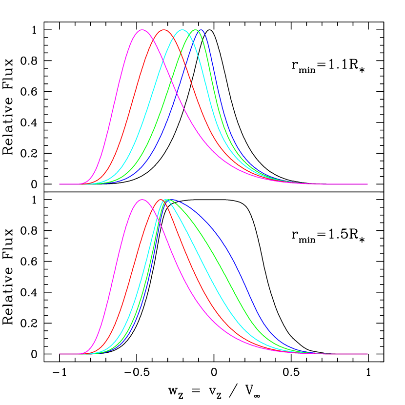
Figure 6: As in Fig. 5, but now for slower moving clumps with $\beta_{\rm cl}=3$.

The range of line profiles that result in the smooth limiting case are displayed in Figures 5 and 6. A stellar wind terminal speed of $V_{\infty}=2500$ km s^-1 is adopted, as before. For all cases there is a minimum radius (or velocity) in which hot X-ray emitting plasma is to be found. For the upper panels, the radius is $r_{\rm min}=1.1R_{\ast}$, and for the lower panels, it is $r_{\rm min}=1.5R_{\ast}$. The two left panels are profiles that result for fast clumps with $\beta_{\rm cl}=0.5$; the two right panels are for slow clumps with $\beta_{\rm cl}=3$.

The line emission is assumed to be optically thin (hence no resonance scattering effects). The model line luminosity as a function of relative velocity shift $w_{Z}=v_{Z}/V_{\infty}$ is calculated by

$$L_{\rm line}(w_{Z})=\int_{w_{Z}}\,\Lambda(T)\,\frac{dEM}{dT}\,e^{-\tau}\,dT$$ (30)

where $\Lambda(T)$ is the temperature dependent line cooling function, $\tau$ is the photoabsorption optical (see below), and the integral is carried out over the unocculted volume. For initial calculations we assume simply that $\Lambda(T)$ is a constant. We also ignore the variation of ion fraction with $T$, implicit in the DEM factor. In effect, these illustrative model line profiles are meant to sample the full DEM distribution. The inclusion of $T$-dependence for line cooling function and the effects of ionization balance should result in a more diverse set of line profiles.

The different colored curves in Figures 5 and 6 are for different levels of wind photoabsorption. The assumption is that the clumps are small compared to other scales in the problem so that the photoabsorption optical depth $\tau$ is approximated from a LOS integration through a smooth interclump wind. As such, the photoabsorption optical depth to the clump position is the same for all points along the bow shock.

The optical depth is calculated following Ignace (2001), with

$$\tau(r,\vartheta)=\frac{\tau_{\ast}}{r\,\sin\vartheta}\,\int_{0}^{\vartheta}\,\frac{d\vartheta^{\prime}}{1-[(b\sin\vartheta^{\prime})/(r\sin\vartheta)]},$$ (31)

where $\tau_{\ast}$ is the optical depth scale to the base of the wind at $R_{\ast}$. Generally, this scale is related to the wind mass-loss rate, abundances, and energy of the particular line transition in question.

In Figures 5 and 6 profiles for values of $\tau_{\ast}=0,0.5,1,2,4,$ and 8 are calculated. The effect of increasing $\tau_{\ast}$ is to make the profiles increasingly asymmetric with emission peaks of progressively higher blueshifts. The black profile is for a line with $\tau_{\ast}=0$; magneta corresponds to the case of $\tau_{\ast}=8$. Note that with no photoabsorption, the black curve displays a central “flat-top” indicative of $V_{\rm min}=V(r_{\rm min})$, modulo the effect of stellar occultation.

For the range of photoabsorptive optical depths used, the blueshifted peaks all lie below about half of terminal speed. The line widths actually decrease slightly for low $\tau_{\ast}$, but then increase with larger values of $\tau_{\ast}$. Ultimately, at large optical depths, the blueshift of the peak emission and the line width are not sensitive to the value of $r_{\rm min}$.

4.2 The Case of Discrete Clumps

Relaxing the assumption of a smooth distribution of clumps, a discretely structured flow is now considered. Models are based on a random number generator to place clumps throughout the wind from which the X-ray emission line profiles are computed. Let $s$ be a random number in the range of 0 to 1. Individual clumps are sprinkled in a uniformly random way about the star. The $i$th clump will have angular coordinates given by $\varphi_{\rm i}=2\pi s$ and $\mu_{\rm i}=-1+2s$, where $\mu_{\rm i}=\cos\vartheta_{\rm i}$, and of course two distinct random numbers $s$ are used to set the two seperate coordinates for a given clump.

Radial placement requires a different approach. In our model clumps exist exterior to the photospheric level, $R_{\ast}$, out to infinite distance, in principle. The 1D radiative hydrodynamic simulations indicate that the formation of strong shocks occurs primarily at low and intermediate radii in the flow (e.g., Feldmeier, Puls, & Pauldrach 1997), basically where the velocity gradient is reasonably strong. Structure can persist and evolve out to fairly large radius. As a way of capturing the flavor of this scenario, we choose to space clumps such that they are statistically uniformly distributed in radial velocity $V_{W}$. In relation to the preceding section, this means that $dN/dV$ now becomes a uniform probability distribution to be sampled in the range of $V_{0}$ to $V_{\infty}$.

The relationship between a random number $s$ and the corresponding velocity for that value is given by:

$$s=\frac{V_{W}-V_{0}}{V_{\infty}-V_{0}}.$$ (32)

Naturally, this distribution is highly non-uniform in radius. On average half of the clumps lie at $V_{W}>0.5V_{\infty}$, and the other half lie below that speed. For $\beta_{W}=1$, this means that half the clumps lie beyond $r=2R_{\ast}$, and half lie interior. One can easily incorporate different distributions $dN/dV$, either as an exploration of parameter space or to match known clumping properties of a particular source. The manner in which X-ray producing structures are placed in velocity space influences the line profile shape. Our choice of $dN/dV$ as uniform is merely a convenience for purposes of illustration.

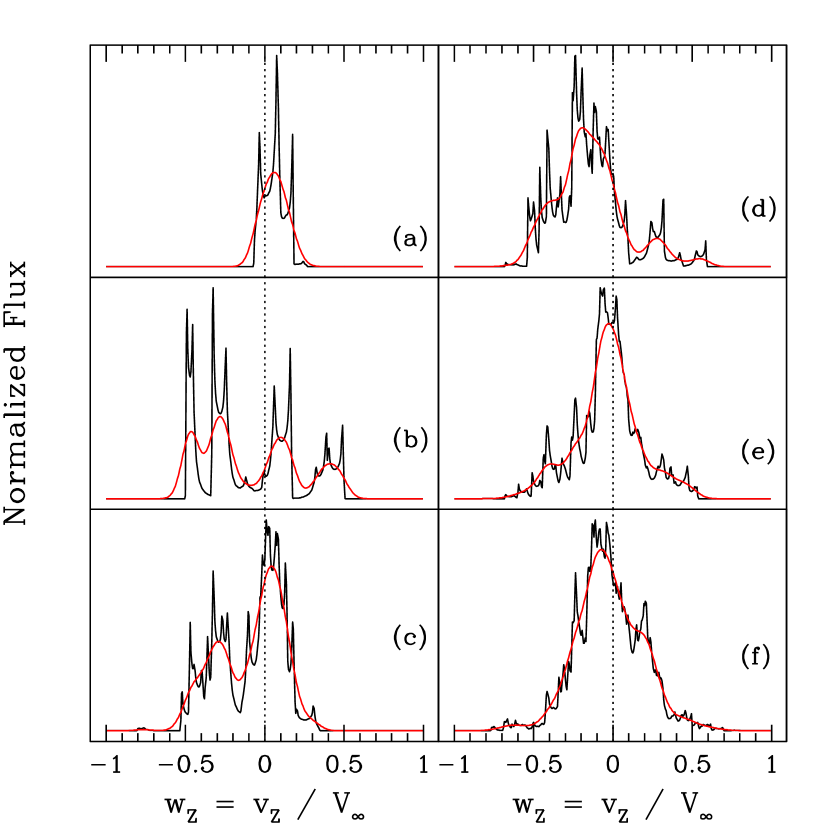
Figure 7: Line profile shapes for an ensemble of clumps with $\tau_{\ast}=0.1$. Panels are distinguished by the number of clumps ${\cal N}_{\rm cl}$ used in the model, with (a) 4, (b) 8, (c) 16, (d) 32, (e) 64, and (f) 128 clumps. Model line profiles are shown in black; overplotted are red curves that include the effects of instrumental smearing are included. Finite spectral resolution is approximated by convolving model lines with a Gaussian that has $\sigma=0.05V_{\infty}$.

Figure 7 shows examples of emission lines for different clump ensembles. The wind photoabsorption optical depth is set to a low value of $\tau_{\ast}=0.1$. All profiles have been normalized to unit area and so no vertical scale of flux is provided. The six panels labelled (a)–(f) correspond to different numbers of clumps ${\cal N}_{\rm cl}$ with 4 in (a), 8 in (b), 16 in (c), 32 in (d), 64 in (e), and 128 in (f). The black curves are the intrinsic profiles of the model calculation, whereas the red curves are convolved by a Gaussian to simulate the effect of instrumental smearing from finite spectral resolution.

It is important to note that the number of clumps contributing to a given profile is generally less than the value of ${\cal N}_{\rm cl}$. This occurs for a couple of reasons. First, we adopt a threshold temperature of 0.5 MK for gas to contribute to the line. If the apex value $T_{A}$ is less than the threshold, then all the gas in the bow shock of that clump is also less than the threshold. The threshold eliminates those clumps that are very near the photosphere and very far away, where $\Delta V$ is too small to generate the requisite temperatures for X-ray emission. The second reason is that some clumps are occulted.

With ${\cal N}_{\rm cl}$ on the order of several tens and higher, the convolved profiles are reasonably symmetric (but not exactly so). Of course the extent of blueshifted peak emission and line width is a function of photoabsorption optical depth.

We have not properly dealt with the fact that there is generally a broad range of temperatures across the bow shock. The emission lines of Figure 7 still adopt a temperature independent line emissivity as was used for the effectively smooth wind case of section 4.1. A temperature dependent emissivity should be included when fitting observed line profiles for specific sources.

5 Summary and Conclusions

Paper I of this series presented results of a hydrodynamic simulation for purely adiabatic cooling with a plane-parallel hypersonic flow impinging upon a rigid spherical obstacle in the rest frame of that obstacle. The simulation was conducted under the assumption that individual clump structures are much smaller than the radius at which they are located. In that paper the flow and temperature structure were described, and two quite interesting simplifications were emphasized. First, it was found that the DEM followed a power-law form. Second, the emission measure was to be found primarily in a thin “sheath” of postshock volume. Thus Cassinelli et al. (2008) introduced the on-the-shock approximation, or “OTSh”, whereby the bow shock geometry determines the $T$ and $DEM$ distributions necessary for computing observables.

In this second paper, we adopt the OTSh to model X-ray emission lines that would arise from an individual bow shock and from an ensemble of bow shocks. This follows on a long string of papers to explain the unexpected observed X-ray line profile shapes from a number of massive stars in terms of structured flows, based on fragments of planar shocks (Oskinova et al. 2004) or porosity arguments (Owocki & Cohen 2006).

An individual clump tends to produce an asymmetric double-horned emission profile that is offset from line center, depending on its radial and lateral location around the star from the observer. Evidence indicates that massive star winds are characterized by large numbers of clump structures. To model the line shapes from an ensemble of clumps, we adopted a parametric two-component flow approach using two wind $\beta$-laws: one for the interclump wind flow and one for the clump flow. The distinction in $\beta$-laws leads to radius-dependent velocity jumps that govern the temperature range of the bow shocks. Of particular interest is that this approach yields a number of semi-analytic relationships for the $T$ and DEM distributions throughout the flow, which in principle are properties that can be tested against observations (e.g., Waldron & Cassinelli 2009; Guo 2010);

Using this construction, emission line profiles were calculated in the “smooth” limit of many uniformly distributed clumps and for the case of a discretely structured flow. As expected, peak emission of the lines are a function of the degree of photoabsorption. The bow shock paradigm yields line shapes that are somewhat symmetric at modest photoabsorption optical depths of a few, where the influence of $r_{\rm min}$ on the line shape can no longer be perceived. In contrast to a uniform distribution of clumps, the discrete case leads to profiles with spikey features; however, these are much too narrow to actually resolve with current instrumentation. Using a simple temperature cut-off approach, we also find that profile widths can depend on the temperature interval of line formation.

All of these results represent a promising starting point for tailored analyses of individual objects, for calculating spectral energy distributions, and for investigating X-ray variability. Previous efforts have focused primarily on geometrical considerations for explaining X-ray line profiles shapes observed from OB stars, in the form of discrete clumps, clump distributions, and/or filling factor considerations. Our results explicitly include temperature distributions throughout the wind flow, which is a forward step in X-ray line profile synthesis modeling.

In closing we remind the reader that our approach has relied on simulations that adopt purely adiabatic cooling for the bow shocks. We have begun new simulations of clump bow shocks that include radiative cooling. The advantage of adiabatic cooling and hypersonic flow is that the flow geometry is independent of the Mach number. In situations where radiative cooling is needed, the results will depend on the density and the apex temperature achieved. Consequently, the bow shock structure will no longer have a “universal” form; thus, greater complexity is the cost of greater realism. Preliminary results with radiative cooling suggest that the power-law DEM in temperature derived in Paper I persists at the hottest temperatures, but shows a flattening toward cooler temperature gas where radiative cooling dominates. In the future we will include the results of these new simulations along with realistic temperature-dependent line emissivities to fit the line profiles of high resolution X-ray lines from massive star winds and to study time variable effects of X-ray emissions.

Appendix A Appendix: Temperature Intervals for $\beta_{\rm cl}=1/2$, 2, and 3

To calculate the total DEM from a uniform distribution of many clumps in a wind, it is necessary to find the integration limits $w_{1}(T)$ and $w_{2}(T)$ in eq. (4.1). Based on the preceding section, this amounts to a root finding exercise involving the following relation (see eq. [22]):

$$w^{\beta_{\rm cl}}-w+\sqrt{t}=0,$$ (A1)

where $t=T/T_{\rm lim}$ and $\beta_{W}=1$ is assumed. The function is double-valued for all $\beta_{\rm cl}\neq 1$. Note that the clump $\beta_{\rm cl}$ can be larger or smaller than the interclump value. Here solutions are given for three cases where the roots are analytic or semi-analytic.

A.1 Case of $\beta_{\rm cl}=2$

The equation to be solved is

$$w^{2}-w+\sqrt{t}=0.$$ (A2)

The roots have with values of

$$w_{1,2}=\frac{1}{2}\mp\frac{1}{2}\,\sqrt{1-4\sqrt{t}}.$$ (A3)

The maximum temperature occurs at $t_{\rm max}=1/16$ for which $w_{1}=w_{2}=0.5$.

A.2 Case of $\beta_{\rm cl}=1/2$

The equation to be solved is

$$w-\sqrt{w}+\sqrt{t}=0.$$ (A4)

With the change of variable $x^{2}=w$, the condition can be recast as

$$x^{2}-x+\sqrt{t}=0,$$ (A5)

which is the same quadratic expression for $\beta_{\rm cl}=2$. The roots $w_{1,2}$ for the case $\beta_{\rm cl}=1/2$ are simply the square roots of the solutions from the $\beta_{\rm cl}=2$ case. The maximum temperature still occurs at $t_{\rm max}=1/16$, which in velocity is now $w_{1}=w_{2}=0.25$.

A.3 Case of $\beta_{\rm cl}=3$

The expression to be solved is

$$w^{3}-w+\sqrt{t}=0.$$ (A6)

This cubic has three real roots; however, one of those is negative and not physical. There are standard forms for the roots; here we use the trigonometric version. An angle $\gamma$ is introduced as defined by

$$\cos\gamma=-\sqrt{t/t_{\rm max}},$$ (A7)

where $t_{\rm max}=4/27$. Then the roots become

$$w_{2}=\frac{2}{\sqrt{3}}\,\cos(\gamma/3),$$ (A8)

and

$$w_{1}=\sqrt{1-\frac{3}{4}\,w_{2}^{2}}-\frac{1}{2}\,w_{2}.$$ (A9)

References

- (1)
- (2) Berghoefer, T. W., Schmitt, J. H. M. M., 1994, A&A, 290, 435
- (3) Berghoefer, T. W., Baade, D., Schmitt, J. H. M. M., Kudritzski, R.-P., Puls, J., et al., 1996, A&A, 306, 899
- (4) Berghoefer, T. W., Schmitt, J. H. M. M., Danner, R., Cassinelli, J. P., 1997, A&A, 322, 167
- (5) Brown, J. C., McLean, I. S., 1977, A&A, 57, 141
- (6) Brown, J. C., Ignace, R., Cassinelli, J. P., 2000, A&A, 356, 619
- (7) Cassinelli, J. P., et al., 1981, ApJ, 250, 677
- (8) Cassinelli, J. P., Castor, J. I., Lamers, J. G. L. M., 1978, PASP, 90, 496
- (9) Cassinelli, J. P., Ignace, R., Waldron, W. L., Cho, J., Murphy, N. A., Lazarian, A., 2008, ApJ, 683, 1052 [Paper I]
- (10) Cassinelli, J. P., Miller, N. A., Waldron, W. L., MacFarlane, J. J., Cohen, D. H., 2001, ApJ, 554, L55
- (11) Cassinelli, J. P. & Olson, G. L., 1979, ApJ, 229, 304
- (12) Cassinelli, J. P. & Swank, J. H. 1983, ApJ, 271, 681
- (13) Clarke, D., McDavid, D., Smith, R. A., Henrichs, H. F., 2002, A&A, 383, 580
- (14) Dessart, L., Owocki, S. P., 2003, A&A, 406, L1
- (15) Dessart, L., Owocki, S. P., 2005, A&A, 437, 657
- (16) Feldmeier, A., 1995, A&A, 299, 523
- (17) Feldmeier, A., Puls, J., & Pauldrach, A. W. A. 1997, 322, 878
- (18) Feldmeier, A., Oskinova, L., & Hamann, W. -R. 2003, A&A, 403, 217
- (19) Fullerton, A. W., Massa, D. L., Prinja, R. K., 2006, ApJ, 637, 1025
- (20) Güdel, M., Nazé, Y., 2009, A&A Reviews, 17, 309
- (21) Guo, J. H., 2010, A&A, 512, 50
- (22) Hamann, W.-R., Koesterke, L., 1998, A&A, 335, 1003
- (23) Harnden, F. R., Jr., et al., 1979, ApJ, 234, L51
- (24) Hayes, W. D., Probstein, R. F. 2004, Hypersonic Inviscid Flow (Dover: Mineola, NY)
- (25) Hillier, D. J., 1991, A&A, 247, 455
- (26) Hole, K. T., Ignace, R., 2012, A&A, accepted
- (27) Howk, J. C., Cassinelli, J. P., Bjorkman, J. E., & Lamers, H. J. G. L. M. 2000, ApJ, 534, 348
- (28) Ignace, R., 2001, ApJ, 549, L119
- (29) Ignace, R., & Gayley, K., 2002, ApJ, 568, 594
- (30) Kahn, S. M., et al., 2001, A&A, 365, L312
- (31) Lepine, S., Moffat, A. F. J., 1999, ApJ, 514, 909
- (32) Lepine, S., Moffat, A. F. J., 2008, AJ, 136, 548
- (33) Leutenegger, M. A., Paerels, F. B. S., Kahn, S. M., Cohen, D. H., 2006, ApJ, 650, 1096
- (34) Leutenegger, M. A., Owocki, S. P., Kahn, S. M., Paerels, F. B. S., 2007, ApJ, 659, 642
- (35) Lucy, L. B. 1982, ApJ, 255, 286
- (36) Lucy, L. B., & White, R. L., 1980, ApJ, 241, 300
- (37) Lupie, O. L., Nordsieck, K. H., 987, AJ, 9, 214
- (38) MacFarlane, J. J., Cassinelli, J. P., Welsh, B. Y., Vedder, P. W., Vallerga, J. V., & Waldron, W. L. 1991, ApJ, 380, 564
- (39) McDavid, D., 2000, AJ, 119, 352
- (40) Miller, N. A., Cassinelli, J. P., Waldron, W. L., MacFarlane, J. J., Cohen, D. H., 2002, ApJ, 577, 951
- (41) Moffat, A. F. J., Drissen, L., Lamontagne, R., Carmelle, R., 1988, ApJ, 334, 1038
- (42) Moffat, A. F. J., Robert, C., 1994, ApJ, 421, 310
- (43) Muijres, L. E., de Koter, A., Vink, J. S., Krticka, J., Kubat, J., Langer, N., 2011, A&A, 526, 32
- (44) Mullan, D. J., Waldron, W. L, 2006, ApJ, 637, 506
- (45) Nazé, Y, et al., 2011, ApJS, 194, 7
- (46) Nichols, J., Mitschang, A. W., Waldron, W., 2011, BAAS, 43, 154.10
- (47) Oskinova, L. M., Feldmeier, A., & Hamann, W.-R. 2004, A&A, 422, 675
- (48) Oskinova, L. M., Feldmeier, A., Hamann, W.-R., 2006, MNRAS, 372, 313
- (49) Oskinova, L. M., Hamann, W.-R., Feldmeier, A., 2007, A&A, 476, 1331
- (50) Owocki, S. P., Castor, J. I., & Rybicki, G. B. 1988, ApJ, 335, 914
- (51) Owocki, S. P., Cohen, D. H., 1999, ApJ, 520, 833
- (52) Owocki, S. P., Cohen, D. H., 2001, ApJ, 559, 1108
- (53) Owocki, S. P., Cohen, D. H., 2006, ApJ, 648, 565
- (54) Owocki, S. P., Sundqvist, J., Cohen, D., Gayley, K., 2011, to appear in Four Decades of Research on Massive Stars, (eds) L. Drissen, C. Robert, N. St.-Louis, (ASP Conf. Ser.), astroph/1110.0891
- (55) Pollock, A., 2007, A&A, 463, 1111
- (56) Prinja, R. K., Massa, D. L., 2010, A&A, 521, L55
- (57) Seward, F. D., et al., 1979, ApJ, 234, L55
- (58) Sundqvist, J. O., Owocki, S. P., Puls, J., 2011, to appear in Four Decades of Research on Massive Stars, (eds) L. Drissen, C. Robert, N. St.-Louis, (ASP Conf. Ser.), astroph/1110.0485
- (59) Walborn, N. R., Nichols, J. S., Waldron, W. L., 2009, ApJ, 703, 633
- (60) Waldron, W. L. & Cassinelli, J. P. 2001, ApJ, 548, L45
- (61) Waldron, W. L., Cassinelli, J. P., 2007, ApJ, 668, 456
- (62) Waldron, W. L., Cassinelli, J. P., 2009, ApJ, 692, L76
- (63) Waldron, W. L., Cassinelli, J. P., 2010, ApJ, 711, L30
- (64)