Constraining Form Factors with the Method of Unitarity Bounds

Abstract

The availability of a reliable bound on an integral involving the square of the modulus of a form factor on the unitarity cut allows one to constrain the form factor at points inside the analyticity domain and its shape parameters, and also to isolate domains on the real axis and in the complex energy plane where zeros are excluded. In this lecture note, we review the mathematical techniques of this formalism in its standard form, known as the method of unitarity bounds, and recent developments which allow us to include information on the phase and modulus along a part of the unitarity cut. We also provide a brief summary of some results that we have obtained in the recent past, which demonstrate the usefulness of the method for precision predictions on the form factors.

1 Introduction

Form factors are basic observables in strong interaction dynamics. They provide information on the nature of the strong force and confinement. The pion electromagnetic form factor is one such observable. The weak form factors are of crucial importance for the determination of standard model parameters such as the elements of the Cabibbo-Kobayashi-Maskawa (CKM) matrix.

Before the advent of the modern theory of strong interactions, mathematical methods were advanced to obtain bounds on the form factors when a suitable integral of the modulus squared along the unitarity cut $(t_{+},\infty)$ was available [1, 2] (for a topical review of the results at that time, see [3]). Using the methods of complex analysis, this condition leads to constraints on the values at points inside the analyticity domain or on the derivatives at $t=0$, such as the slope and curvature. Also of interest was whether or not the form factors can vanish on the real energy or in the complex energy plane (in the context of the pion electromagnetic form factor, see, e.g. [4]). Mathematically, these problems belong to a class referred to as the Meiman problem [5].

At present, effective theories of strong interactions, like Chiral Perturbation Theory (ChPT) or Heavy Quark Effective Theories (HQET), as well as lattice calculations or various types of QCD sum rules, allow us to make predictions, sometimes very precise, on the form factors at particular kinematical regions. However, a full calculation of the hadronic form factors from first principles is not yet possible. On the other hand, experimental information on the form factors has improved considerably in recent years. In these circumstances, analytic techniques as those mentioned above prove to be very useful, providing rigorous correlations and consistency checks of various approaches and in improving the phenomenological analyses of the form factors. In a recent review, ref. [6] we have presented a complete treament of the mathematical background required for studying these problems and a comprehensive bibliography on the subject.

The integral condition was provided either from an observable (like muon’s $g-2$ in the case of the electromagnetic form factor of the pion) or, in the modern approach first applied in [7], from the dispersion relation satisfied by a suitable correlator calculated by perturbative QCD in the spacelike region, and whose positive spectral function has, by unitarity, a lower bound involving the modulus squared of the relevant form factor. Therefore, the constraints derived in this framework are often referred to as “unitarity bounds”. Information about the phase of the form factor, available by Watson’s theorem from the associated elastic scattering, can be used to improve the results in a systematic fashion [8, 9]. In some cases the modulus is also measured independently along a part of the unitarity cut.

Recent applications in the modern approach concerned mainly the form factors relevant for the $B\to D^{(*)}$ semileptonic decays, or the so-called Isgur-Wise function, where heavy quark symmetry provided strong additional constraints at interior points [10, 11, 12, 13, 14, 15]. More recent applications revisited the electromagnetic form factor of the pion [16, 17, 18, 19, 20], the strangeness changing $K\pi$ form factors [21, 22, 23, 24, 25], the $B\pi$ vector form factor [26, 27, 28], and also the $D\pi$ form factors [29]. The results confirm that the approach represents a useful tool in the study of the form factors, complementary and free of additional assumptions inherent in standard dispersion relations. The techniques presented here are the framework of including inputs coming from disparate sources and effectively testing their consistency. In this lecture note we will describe the mathematical machinery that has been developed to address these issues. We will also review some recent results obtained by us using these methods.

In Sec. 2 we present our notation and describe the general Meiman interpolation problem, for an arbitrary number of derivatives at the origin and an arbitrary number of values at points inside the analyticity domain. The solution is obtained by Lagrange multipliers, and is written as a positivity condition of a determinant written down in terms of the input values. Alternatively, using techniques of analytic interpolation theory, the result can be written as a compact convex quadratic form, given in ref. [6]. We present the complete treatment of the inclusion of the phase on a part of the unitarity cut, ($t_{+},t_{\rm in})$, along with an arbitrary number of constraints of the Meiman type in Sec. 3. The general treatment was only recently provided in entirety despite the lengthy literature on the problem. Two equivalent sets of integral equations have been found and here we provide the result obtained from using the method of Lagrange multipliers. The result obtained from analytic interpolation theory can be found in [6]. In Sec. 4 we treat a modified analytic optimization problem, where the input on the cut consists from the phase below a certain threshold $t_{\rm in}$ and a weighted integral over the modulus squared along $t>t_{\rm in}$. This is a mathematically more complicated problem solved for the first time in [16]. The method uses the fact that the knowledge of the phase allows one to describe exactly the elastic cut of the form factor by means of the Omnès function. The problem is thus reduced to a standard Meiman problem on a larger analyticity domain. In practice, the integral along $t>t_{\rm in}$ can be obtained by subtracting from the integral along the whole cut the low-energy contribution, $t<t_{\rm in}$, which can be estimated if some information on the modulus on that part of the cut is available from an independent source. The integral can be evaluated also if precise data on the modulus are available up to high energies, as is the case with the pion electromagnetic form factor [30, 31]. In Sec. 5 we present for illustration most recent results of these methods applied to the pion electromagnetic form factor [20]. We conclude with an afterword, Sec. 6.

2 Meiman Problem

In order to set up the notation, let us begin by letting $F(t)$ denote a form factor, which is real analytic (i.e. $F(t^{*})=F^{*}(t)$) in the complex $t$-plane with a cut along the positive real axis from the lowest unitarity branch point $t_{+}$ to $\infty$. The essential condition considered in the present context is an inequality:

$$\int^{\infty}_{t_{+}}dt\ \rho(t)|F(t)|^{2}\leq I,$$ (1)

where $\rho(t)\geq 0$ is a positive semi-definite weight function and $I$ is a known quantity. As mentioned in the Introduction, such inequalities can be obtained starting from a dispersion relation satisfied by a suitable correlator, evaluated in the deep Euclidean region by perturbative QCD, and whose spectral function is bounded from below by a term involving the modulus squared of the relevant form factor.

Of interest in the analysis of form factors are the shape parameters that appear in the expansion around $t=0$. For instance, in the case of the pion electromagnetic form factor the expansion is customarily written as

$$F(t)=1+\displaystyle\frac{1}{6}\langle r^{2}_{\pi}\rangle t+ct^{2}+dt^{3}+\cdots,$$ (2)

whereas in the analysis of the semileptonic decays, one is interested in the shape parameters appearing in

$$F(t)=F(0)\left[1+\lambda^{\prime}\,\frac{t}{M^{2}}+\lambda^{\prime\prime}\,\frac{t^{2}}{2M^{4}}+\cdots\right],$$ (3)

where $M$ is a suitable mass and $\lambda^{\prime}$ and $\lambda^{\prime\prime}$ denote the dimensionless slope and curvature, respectively.

Low energy theorems, reflecting the chiral symmetry of the strong interaction, and lattice calculations can provide information on $F(t)$ at several special points inside the analyticity domain. The standard unitarity bounds exploit analyticity of the form factor and the inequality (1) in order to correlate in an optimal way these values and the expansion parameters in (3).

In order to set up the stage, the problem is brought to a canonical form by making the conformal transformation

$$\bar{z}(t)=\frac{\sqrt{t_{+}}-\sqrt{t_{+}-t}}{\sqrt{t_{+}}+\sqrt{t_{+}-t}}\,,$$ (4)

that maps the cut $t$-plane onto the unit disc $|z|<1$ in the $z\equiv\bar{z}(t)$ plane, such that $t_{+}$ is mapped onto $z=1$, the point at infinity to $z=-1$ and the origin to $z=0$. After this mapping, the inequality (1) is written as

$$\frac{1}{2\pi}\int_{0}^{2\pi}{\rm d}\theta|g(e^{i\theta})|^{2}\leq I,$$ (5)

where the analytic function $g(z)$ is defined as

$$g(z)=F(\bar{t}(z))w(z).$$ (6)

Here $\bar{t}(z)$ is the inverse of (4) and $w(z)$ is an outer function, i.e. a function analytic and without zeros in $|z|<1$, such that its modulus on the boundary is related to $\rho(\bar{t}(\e^{i\theta}))$ and the Jacobian of the transformation (4). In particular cases of physical interest, the outer functions $w(z)$ have a simple analytic form. In general, an outer function is obtained from its modulus on the boundary by the integral

$$w(z)=\exp\left[\frac{1}{2\pi}\int_{0}^{2\pi}{\rm d}\theta\,\frac{e^{i\theta}+z}{e^{i\theta}-z}\,\ln|w(e^{i\theta})|\right].$$ (7)

The function $g(z)$ is analytic within the unit disc and can be expanded as:

$$g(z)=g_{0}+g_{1}z+g_{2}z^{2}+\cdots,$$ (8)

and (5) implies

$$\sum_{k=0}^{\infty}g_{k}^{2}\leq I.$$ (9)

Using (6), the real numbers $g_{k}$ are expressed in a straightforward way in terms of the coefficients of the Taylor expansion (3). The inequality (9), with the sum in the left side truncated at some finite order, represents the simplest “unitarity bound” for the shape parameters defined in (3). In what follows we shall improve it by including additional information on the form factor.

We consider the general case when the first $K$ derivatives of $g(z)$ at $z=0$ and the values at $N$ interior points are assumed to be known:

$$\left[\displaystyle\frac{1}{k!}\displaystyle\frac{d^{k}g(z)}{dz^{k}}\right]_{z=0} = g_{k},\quad 0\leq k\leq K-1;$$

$$g(z_{n}) = \xi_{n},\quad 1\leq n\leq N,$$ (10)

where $g_{k}$ and $\xi_{n}$ are given numbers. They are related, by (6), to the derivatives $F^{(j)}(0)$, $j\leq k$ of $F(t)$ at $t=0$, and the values $F(\bar{t}(z_{n}))$, respectively. For simplicity and in view of phenomenological inputs that we will use, we assume the points $z_{n}$ to be real, so $\xi_{n}$ are also real. The Meiman problem requires to find the optimal constraints satisfied by the numbers defined in (2) if (5) holds. One can prove that the most general constraint satisfied by the input values appearing in (2) is given by the inequality:

$$\mu_{0}^{2}\leq I,$$ (11)

where $\mu_{0}^{2}$ is the solution of the minimization problem:

$$\mu_{0}^{2}=\min\limits_{g\in{\cal G}}\,||g||^{2}_{L^{2}}.$$ (12)

Here $||g||_{L^{2}}^{2}$ denotes the $L^{2}$ norm, i.e. the quantity appearing in the l.h.s. of (5) or (9), and the minimum is taken over the class ${\cal G}$ of analytic functions which satisfy the conditions (2).

The minimization problem (12) can be solved by using the Lagrange multiplier method. The Lagrangian may be written as

$${\cal L}=\frac{1}{2}\sum_{k=0}^{\infty}g_{k}^{2}+\sum_{n=1}^{N}\alpha_{n}(\xi_{n}-\sum_{k=0}^{\infty}g_{k}z^{k}),$$ (13)

where $\alpha_{n}$ are real Lagrange multipliers. Solving the Lagrange equations obtained by varying with respect to $g_{k}$ for all $k\geq K$, and eliminating the Lagrange multipliers yields the solution of the minimization problem (12). For purposes of illustration, when $N=2$, the Lagrange equations yield

$$g_{k}=\alpha_{1}z_{1}^{k}+\alpha_{2}z_{2}^{k},\quad\quad k\geq K,$$ (14)

and the inequality (11) can be expressed in terms of the two Lagrange multipliers as:

$$\alpha_{1}\bar{\xi}_{1}+\alpha_{2}\bar{\xi}_{2}\,\leq\,\bar{I},$$ (15)

where $\bar{\xi}_{n}$ are known numbers defined as

$$\bar{\xi}_{n}=\xi_{n}-\sum_{k=0}^{K-1}g_{k}z_{n}^{k},$$ (16)

and

$$\bar{I}=I-\sum_{k=0}^{K-1}g_{k}^{2}.$$ (17)

The constraint conditions themselves are

$$\displaystyle\alpha_{1}\frac{z_{1}^{2K}}{1-z_{1}^{2}}+\alpha_{2}\frac{(z_{1}z_{2})^{K}}{1-z_{1}z_{2}}=\bar{\xi}_{1},$$

$$\displaystyle\alpha_{1}\frac{(z_{1}z_{2})^{K}}{1-z_{1}z_{2}}+\alpha_{2}\frac{z_{2}^{2K}}{1-z_{2}^{2}}=\bar{\xi}_{2}.$$ (18)

The consistency of eqs. (15) and (2) as a system of equations for $\alpha_{i}$ can be written as:

$$\left|\begin{array}[]{c c c}\bar{I}&\bar{\xi}_{1}&\bar{\xi}_{2}\\ \bar{\xi}_{1}&\displaystyle\frac{z_{1}^{2K}}{1-z_{1}^{2}}&\displaystyle\frac{(z_{1}z_{2})^{K}}{1-z_{1}z_{2}}\\ \bar{\xi}_{2}&\displaystyle\frac{(z_{1}z_{2})^{K}}{1-z_{1}z_{2}}&\displaystyle\frac{z_{2}^{2K}}{1-z_{2}^{2}}\\ \end{array}\right|\geq 0.$$ (19)

This can be readily extended to the case of $N$ constraints:

$$\left|\begin{array}[]{c c c c c c}\bar{I}&\bar{\xi}_{1}&\bar{\xi}_{2}&\cdots&\bar{\xi}_{N}\\ \bar{\xi}_{1}&\displaystyle\frac{z^{2K}_{1}}{1-z^{2}_{1}}&\displaystyle\frac{(z_{1}z_{2})^{K}}{1-z_{1}z_{2}}&\cdots&\displaystyle\frac{(z_{1}z_{N})^{K}}{1-z_{1}z_{N}}\\ \bar{\xi}_{2}&\displaystyle\frac{(z_{1}z_{2})^{K}}{1-z_{1}z_{2}}&\displaystyle\frac{(z_{2})^{2K}}{1-z_{2}^{2}}&\cdots&\displaystyle\frac{(z_{2}z_{N})^{K}}{1-z_{2}z_{N}}\\ \vdots&\vdots&\vdots&\vdots&\vdots\\ \bar{\xi}_{N}&\displaystyle\frac{(z_{1}z_{N})^{K}}{1-z_{1}z_{N}}&\displaystyle\frac{(z_{2}z_{N})^{K}}{1-z_{2}z_{N}}&\cdots&\displaystyle\frac{z_{N}^{2K}}{1-z_{N}^{2}}\\ \end{array}\right|\geq 0.$$ (20)

Alternatively, the solution can be obtained by introducing Lagrange multipliers also for the given coefficients $g_{k},\,k=0,...,K-1$ in (13). This leads to an inequality, equivalent to (20), written as [32]:

$$\left|\begin{array}[]{c c c c c c c c c}I&g_{0}&g_{1}&\cdots&g_{K-1}&\xi_{1}&\xi_{2}&\cdots&\xi_{N}\\ g_{0}&1&0&0&0&1&1&\cdots&1\\ g_{1}&0&1&0&0&z_{1}&z_{2}&\cdots&z_{N}\\ \vdots&\vdots&\vdots&\vdots&\vdots&\vdots&\vdots&\vdots&\\ g_{K-1}&0&0&\cdots&1&z_{1}^{K-1}&z_{2}^{K-1}&\cdots&z_{N}^{K-1}\\ \xi_{1}&1&z_{1}&\cdots&z_{1}^{K-1}&\frac{1}{1-z_{1}^{2}}&\frac{1}{1-z_{1}z_{2}}&\cdots&\frac{1}{1-z_{1}z_{N}}\\ \xi_{2}&1&z_{2}&\cdots&z_{2}^{K-1}&\frac{1}{1-z_{1}z_{2}}&\frac{1}{1-z_{2}^{2}}&\cdots&\frac{1}{1-z_{2}z_{N}}\\ \vdots&\vdots&\vdots&\vdots&\vdots&\vdots&\vdots&\vdots&\\ \xi_{N}&1&z_{N}&\cdots&z_{N}^{K-1}&\frac{1}{1-z_{1}z_{N}}&\frac{1}{1-z_{2}z_{N}}&\cdots&\frac{1}{1-z_{N}^{2}}\\ \end{array}\right|\geq 0.$$ (21)

The conditions (20) or (21) can be expressed in a straightforward way in terms of the values of the form factor $F(t)$ at $t_{i}=\bar{t}(z_{i})$ and the derivatives at $t=0$, using eqs. (4) and (6). It can be shown that these inequalities define convex domains in the space of the input parameters.

3 Inclusion of Phase Information

Additional information on the unitarity cut can be included in the formalism. According to the Fermi-Watson theorem, below the inelastic threshold $t_{\rm in}$ the phase of $F(t)$ is equal (modulo $\pi$) to the phase $\delta(t)$ of the associated elastic scattering process. Thus,

$$F(t+i\epsilon)=|F(t)|e^{i\delta(t)},\quad\quad t_{+}<t<t_{\rm in},$$ (22)

where $\delta(t)$ is known.

In order to impose the constraint (22), we define first the Omnès function

$${\cal{O}}(t)=\exp\left(\displaystyle\frac{t}{\pi}\int^{\infty}_{t_{+}}dt\displaystyle\frac{\delta(t^{\prime})}{t^{\prime}(t^{\prime}-t)}\right),$$ (23)

where $\delta(t)$ is known for $t\leq t_{\rm in}$, and is an arbitrary function, sufficiently smooth (i.e. Lipschitz continuous) for $t>t_{\rm in}$. From (22) and (23) it follows that

$${\rm Im}\left[\frac{F(t+i\epsilon)}{{\cal{O}}(t+i\epsilon)}\right]=0,\quad\quad t_{+}\leq t\leq t_{\rm in}.$$ (24)

Expressed in terms of the function $g(z)$ this condition becomes

$${\rm Im}\left[\frac{g(e^{i\theta})}{W(\theta)}\right]=0,\quad\quad\theta\in(-\theta_{\rm in},\theta_{\rm in}).$$ (25)

Here $\theta_{\rm in}$ is defined by $\bar{z}(t_{\rm in})=\exp(i\theta_{\rm in})$ and the function $W(\theta)$ is defined as:

$$W(\theta)=w(e^{i\theta})O(e^{i\theta}),$$ (26)

where $w(z)$ is the outer function and

$$O(z)={\cal{O}}(\bar{t}(z)).$$ (27)

The constraint (25) can be imposed by means of a generalized Lagrange multiplier, while constraints at interior points can be treated with standard real-valued Lagrange multipliers. The Lagrangian of the minimization problem (12) with the constraints (2) and (25) reads

$${\cal L} = \frac{1}{2}\sum_{k=0}^{\infty}g_{k}^{2}+\sum_{n=1}^{N}\alpha_{n}(\xi_{n}-\sum_{k=0}^{\infty}g_{k}z^{k})$$

$$+ \frac{1}{\pi}\sum_{k=0}^{\infty}g_{k}\lim_{\rm r\rightarrow 1}\int\limits_{-\theta_{\rm in}}^{\theta_{\rm in}}\lambda(\theta^{\prime})|W(\theta^{\prime})|{\rm{Im}}[[W(\theta^{\prime})]^{-1}r^{k}e^{ik\theta^{\prime}}]d\theta^{\prime}.$$

The Lagrange multiplier $\lambda(\theta)$ is an odd function, $\lambda(-\theta)=-\lambda(\theta)$ and the factor $|W(\theta^{\prime})|$ was introduced in the integrand for convenience.

We minimize ${\cal L}$ by brute force method with respect to the free parameters $g_{k}$ with $k\geq K$. The Lagrange multipliers $\lambda(\theta)$ and $\alpha_{n}$ are found in the standard way by imposing the constraints (2) and (25).

The calculations are straightforward. In order to write the equations in a simple form, it is convenient to define the phase $\Phi(\theta)$ of the function $W(\theta)$ by

$$W(\theta)=|W(\theta)|e^{i\Phi(\theta)}.$$ (29)

From (26) we have

$$\Phi(\theta)=\phi(\theta)+\delta(\tilde{t}(e^{i\theta})),$$ (30)

where $\phi(\theta)$ is the phase of the outer function $w(e^{i\theta})$ and $\delta(t)$ is the elastic scattering phase shift. We introduce also the functions $\beta_{n}$ for $n=1,...N$, by

$$\beta_{n}(\theta)=z_{n}^{K}\,\frac{\sin[K\theta-\Phi(\theta)]-z_{n}\sin[(K-1)\theta-\Phi(\theta)]}{1+z_{n}^{2}-2z_{n}\cos\theta}.$$ (31)

Then the equations for the Lagrange multipliers $\lambda(\theta)$ and $\alpha_{n}$ take the form:

$$\sum_{k=0}^{K-1}g_{k}\sin[k\theta-\Phi(\theta)]=\lambda(\theta)-\sum_{n=1}^{N}\alpha_{n}\beta_{n}(\theta)$$ (32)

$$-\frac{1}{2\pi}\int\limits_{-\theta_{\rm in}}^{\theta_{\rm in}}{\rm d}\theta^{\prime}\lambda(\theta^{\prime})){\cal K}_{\Phi}(\theta,\theta^{\prime}),\quad\quad\theta\in(-\theta_{\rm in},\theta_{\rm in}),$$

$$-\frac{1}{\pi}\int\limits_{-\theta_{\rm in}}^{\theta_{\rm in}}\lambda(\theta)\beta_{n}(\theta){\rm d}\theta+\sum_{n^{\prime}=1}^{N}\alpha_{n^{\prime}}\frac{(z_{n}z_{n^{\prime}})^{K}}{1-z_{n}z_{n^{\prime}}}=\bar{\xi}_{n},$$ (33)

where $n=1,\ldots N$.

The integral kernel in (32), defined as

$${\cal K}_{\Phi}(\theta,\theta^{\prime})\equiv\frac{\sin[(K-1/2)(\theta-\theta^{\prime})-\Phi(\theta)+\Phi(\theta^{\prime})]}{\sin[(\theta-\theta^{\prime})/2]},$$ (34)

is of Fredholm type if the phase $\Phi(\theta)$ is Lipschitz continuous Then the above system can be solved numerically in a straightforward manner. Finally, the inequality (11) takes the form:

$$\frac{1}{\pi}\sum_{k=0}^{K-1}g_{k}\int\limits_{-\theta_{\rm in}}^{\theta_{\rm in}}{\rm d}\theta\lambda(\theta)\sin\left[k\theta-\Phi(\theta)\right]+\sum_{n=1}^{N}\alpha_{n}\bar{\xi}_{n}\leq\bar{I},$$ (35)

with $\bar{I}$ defined in (17). Using the relation (6), the above inequality defines an allowed domain for the values of the form factor and its derivatives at the origin. It must be emphasized that the theory for arbitrary number of constraints was presented for the first time in ref. [6]. It is easy to see that, if $t_{\rm in}$ is increased, the allowed domain defined by the inequality (35) becomes smaller. The reason is that by increasing $t_{\rm in}$ the class of functions entering the minimization (12) becomes gradually smaller, leading to a larger value for minimum $\mu_{0}^{2}$ entering the definition (11) of the allowed domain.

4 A Modified Optimization Problem

In this section we shall present the solution of a modified interpolation problem, where the input consists from the phase condition (22) and the inequality

$$\int_{t_{\rm in}}^{\infty}{\rm d}t\rho(t)|F(t)|^{2}\leq I^{\prime},$$ (36)

where $I^{\prime}$ is known. Unlike the previous condition (1), which involved the whole unitarity cut, we assume now that an integral of the modulus squared along $t>t_{\rm in}$ (or a reliable upper bound on it) is known.

In some cases, the quantity $I^{\prime}$ can be obtained from the inequality (1) and the modulus of the form factor along the elastic part of the unitarity cut, if the latter is available from an independent source, for instance from experiment. Then $I^{\prime}$ is given by

$$I^{\prime}=I-\int^{t_{\rm in}}_{t_{+}}{\rm d}t\rho(t)|F(t)|^{2}<I.$$ (37)

In other cases, like for the pion electromagnetic form factor, $I^{\prime}$ can be estimated directly from experimental data on the modulus at high energies, taking into account also the asymptotic decrease $|F(t)|\sim 1/t$ predicted by perturbative QCD.

Once the conditions (22) and (36) are adopted, one can find the optimal domain allowed for the values and the derivatives of the form factor defined in (2). Below we present the solution of the problem as first described in [16]. We start with the remark that the knowledge of the phase was implemented in the previous section by the relation (24), which says that the function $f(t)$ defined through

$$F(t)=f(t){\cal{O}}(t),$$ (38)

is real in the elastic region, $t_{+}\leq t\leq t_{\rm in}$. In fact, since the Omnès function ${\cal{O}}(t)$ fully accounts for the elastic cut of the form factor, the function $f(t)$ has a larger analyticity domain, namely the complex $t$-plane cut only for $t>t_{\rm in}$. Moreover, (37) implies that $f$ satisfies the condition

$$\int_{t_{\rm in}}^{\infty}{\rm d}t\rho(t)|{\cal{O}}(t)|^{2}|f(t)|^{2}\leq I^{\prime}.$$ (39)

This inequality leads, through the techniques presented in section 2, to constraints on the values of $f$ inside the analyticity domain. It is easy to see that the problem differs from the standard one described there only by the appearance of the additional factor $|{\cal{O}}(t)|^{2}$ in the integral, and the fact that the cut starts now at $t_{\rm in}>t_{+}$.

The problem is brought into a canonical form by the new transformation

$$\tilde{z}(t)=\frac{\sqrt{t_{\rm in}}-\sqrt{t_{\rm in}-t}}{\sqrt{t_{\rm in}}+\sqrt{t_{\rm in}-t}}\,,$$ (40)

which maps the complex $t$-plane cut for $t>t_{\rm in}$ on the unit disc in the $z$-plane defined by $z=\tilde{z}(t)$. Then (39) can be written as

$$\frac{1}{2\pi}\int^{2\pi}_{0}{\rm d}\theta|g(\exp(i\theta))|^{2}\leq I^{\prime},$$ (41)

where the function $g$ is now

$$g(z)=w(z)\,\omega(z)\,F(\tilde{t}(z))\,[O(z)]^{-1}.$$ (42)

Here $w(z)$ is the outer function related to the weight $\rho(t)$ and the Jacobian of the new mapping (40) and $O(z)$ is defined as

$$O(z)={\cal{O}}(\tilde{t}(z)),$$ (43)

where $\tilde{t}(z)$ is the inverse of $z=\tilde{z}(t)$ with $\tilde{z}(t)$ defined in (40), and

$$\omega(z)=\exp\left(\displaystyle\frac{\sqrt{t_{\rm in}-\tilde{t}(z)}}{\pi}\int^{\infty}_{t_{\rm in}}{\rm d}t^{\prime}\displaystyle\frac{\ln|{\cal{O}}(t^{\prime})|}{\sqrt{t^{\prime}-t_{\rm in}}(t^{\prime}-\tilde{t}(z))}\right).$$ (44)

The inequality (41) has exactly the same form as (5), and leads to the constraints (20) or (21) for the values and derivatives of $g(z)$ at interior points. Using (42), these constraints are expressed in terms of the physically interesting values of the form factor $F(t)$.

A remark on the uniqueness is of interest: we recall that the Omnès function ${\cal{O}}(t)$ defined in (23) is not unique, as it involves the arbitrary function $\delta(t)$ for $t>t_{\rm in}$. In section 3 we have seen that the results are not affected by this arbitrariness, as the integral equations involved only the known phase below $t_{\rm in}$. This is true also for the results here: the reason is that a change of the function $\delta(t)$ for $t>t_{\rm in}$ is equivalent with a multiplication of $g(z)$ by a function analytic and without zeros in $|z|<1$ (i.e. an outer function). According to the general theory of analytic functions of Hardy class, the multiplication by an outer function does not change the class of functions used in minimization problems. In our case, the arbitrary function $\delta(t)$ for $t>t_{\rm in}$ enters in both the functions $O(z)$ and $\omega(z)$ appearing in (42), and their ambiguities compensate each other exactly. The independence of the results on the choice of the phase for $t>t_{\rm in}$ is confirmed numerically, for functions $\delta(t)$ that are Lipschitz continuous. The constraints provided by the technique of this section are expected to be quite strong since they result from a minimization on a restricted class of analytic functions, where the second Riemann sheet of the form factor is accounted for explicitly by the Omnès function.

On the other hand, it is easy to see that the fulfillment of the condition (39) does not automatically imply that the original condition (1) is satisfied, and both conditions should be applied in order to reduce the allowed range of the parameters of interest.

The mathematical techniques presented can be adapted in a straightforward way to the problem of zeros. Let us assume that the form factor $F(t)$ has a simple zero on the real axis, $F(t_{0})=0$. We shall use this information in the determinant condition: if the zero is compatible with the remaining information, the inequality can be satisfied. If, on the contrary, the inequality is violated, the zero is excluded. It follows that we can obtain a rigorous condition for the domain of points $z_{0}$ (or $t_{0}$) where the zeros are excluded.

For illustration, assume first that we use as input only the value of the form factor at $t=0$. Then from the argument given above, it follows that the domain of real points $t_{0}$ where the form factor cannot have zeros is described by the inequality [20]

$$\left|\begin{array}[]{c c }I^{\prime}-g_{0}^{2}&-g_{0}\\ -g_{0}&\frac{\tilde{z}(t_{0})^{2}}{1-\tilde{z}(t_{0})^{2}}\\ \end{array}\right|\leq 0.$$ (45)

Here, $I^{\prime}$ is the known bound appearing in (36), $g_{0}=g(0)$ is calculated in terms of the input phase from (42), and $\tilde{z}(t)$ is defined in (40). If we include in addition the value $F(t_{1})$ of the form factor at some point $t_{1}$, the condition reads [20]:

$$\left|\begin{array}[]{c c c }I^{\prime}-g_{0}^{2}&g(\tilde{z}(t_{1}))-g_{0}&-g_{0}\\ g(\tilde{z}(t_{1}))-g_{0}&\frac{\tilde{z}(t_{1})^{2}}{1-\tilde{z}(t_{1})^{2}}&\frac{\tilde{z}(t_{1})\tilde{z}(t_{0})}{1-\tilde{z}(t_{1})\tilde{z}(t_{0})}\\ -g_{0}&\frac{\tilde{z}(t_{1})\tilde{z}(t_{0})}{1-\tilde{z}(t_{1})z(t_{0})}&\frac{\tilde{z}(t_{0})^{2}}{1-\tilde{z}(t_{0})^{2}}\\ \end{array}\right|\leq 0.$$ (46)

5 Recent Applications to the Pion Electromagnetic Form Factor

We will now describe some applications of the methods discussed above. Whilst there has been a long series of applications of these methods to the pion electromagnetic form factor, ref. [20] captures the most stringent results. This is based on the fact that the phase of the form factor is determined up to the $\pi\omega$ threshold ($\sqrt{t_{\rm in}}$=917 MeV) in terms of the $I=1,\,l=1$ partial wave of $\pi\pi$ elastic scattering. We have used the recent parametrization given in ref. [33], which agrees well with the solutions of the Roy equations [34] between threshold and 800 MeV. The modulus $|F(t)|$ has been measured also recently with improved precision by BaBar [30] and KLOE [31] collaborations.

We consider the two-pion contribution to the muon $g-2$, when the weight $\rho(t)$ has the form

$$\rho(t)=\frac{\alpha^{2}M_{\mu}^{2}}{12\pi}\frac{(t-t_{+})^{3/2}}{t^{7/2}}K(t),$$

$$K(t)=\int_{0}^{1}du\,\frac{(1-u)u^{2}}{1-u+M_{\mu}^{2}u^{2}/t}.$$ (47)

The two-pion contribution to muon anomaly was evaluated recently with great precision [35] from the accurate BaBar data on the modulus [30]. In ref. [20] the value of the integral $I^{\prime}$ defined in (36) for the weight (5) and the above choice of $\sqrt{t_{\rm in}}$ was evaluated to be $22.17\times 10^{-10}$.

A concrete application of these methods is one of constraining the shape parameters appearing in (2) using as input the conditions (22) and (36) and the technique described in section 4. We use as input also the precise estimate of the coefficient of the linear term $\langle r^{2}_{\pi}\rangle=(0.435\pm 0.005)\,{\rm fm}^{2}$ given in [36], and additional spacelike data coming from [37, 38], which are given in Table 1, where the first error is statistical and the second is systematic.

Table 1: Spacelike data from [37, 38].

$t$	Value[$\,\text{GeV}^{2}$]	$F(t)$
$t_{1}$	$-1.60$	$0.243\pm 0.012_{-0.008}^{+0.019}$
$t_{2}$	$-2.45$	$0.167\pm 0.010_{-0.007}^{+0.013}$

An illustrative example of the results on the shape parameters $c$ and $d$ is given in Fig. 1.

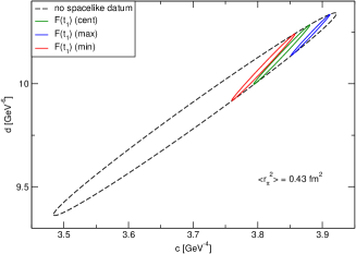
Figure 1: Allowed domain in the $c-d$ plane calculated with $t_{\rm in}=(0.917\,\,\text{GeV})^{2}$ and $\langle r^{2}_{\pi}\rangle=0.43\,{\rm fm}^{2}$, for three values of $F(t_{1})$ at the spacelike point $t_{1}=-1.6\,\,\text{GeV}^{2}$ (central value in Table 1 and the extreme values obtained from the error intervals). Also shown is the large ellipse when no spacelike datum is included.

Varying $F(t_{1})$ given in Table 1 inside the error bars, we obtain the allowed domain of the $c$ and $d$ parameters at the present level of knowledge as the union of the three small ellipses in Fig. 1. By varying also $\langle r^{2}_{\pi}\rangle$ in the range given above the allowed ranges read

$$3.75\,\,\text{GeV}^{-4}\lesssim c\lesssim 3.98\,\,\text{GeV}^{-4},$$

$$9.91\,\,\text{GeV}^{-6}\lesssim d\lesssim 10.45\,\,\text{GeV}^{-6},$$ (48)

with a strong correlation between the two coefficients. Similar results are obtained when the second datum in Table 1 is used in place of the first.

Turning now to the issue of zeros, and using the machinery as described in the preceding section, we find that, for with $\langle r^{2}_{\pi}\rangle=0.43\,{\rm fm}^{2}$, simple zeros are excluded from the interval $-1.93\,\,\text{GeV}^{2}\leq t\leq 0.83\,\,\text{GeV}^{2}$ of the real axis. If we impose the additional constraint at a spacelike point $t_{1}=-1.6\,\,\text{GeV}^{2}$, the interval for the excluded zeros is much bigger. The left end of the range is sensitive to the input value $F_{1}=F(t_{1})$. Using the central value $F_{1}=0.243$ given in Table 1, we find that the form factor cannot have simple zeros in the range $-5.56\,\,\text{GeV}^{2}\leq t\leq 0.84\,\,\text{GeV}^{2}$. By varying $F_{1}$ inside the error interval given in Table 1 (with errors added in quadrature), we find that zeros are excluded from the range $-4.46\,\,\text{GeV}^{2}\leq t\leq 0.84\,\,\text{GeV}^{2}$.

The machinery may now be used to find regions in the complex plane where no zeros are allowed. Complex zeros occur simultaneously at complex conjugate points due to the reality condition. In Fig. 2 we present the exclusion region obtained with central values of the radius and the first datum in Table1. As in the case of the simple zeros on the real axis, there is significant sensitivity to the experimental uncertainty at that point, the allowed region being obtained as the intersection of the regions corresponding to the extreme values. The net effect is a somewhat reduced region compared to that given in Fig. 2.

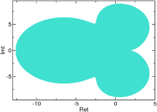
Figure 2: Domain without zeros obtained with $t_{\rm in}=(0.917\,\,\text{GeV})^{2}$ and $\langle r^{2}_{\pi}\rangle=0.43\,{\rm fm}^{2}$, using in addition the central experimental value $F(t_{1})=0.243$ at the spacelike point $t_{1}=-1.6\,\,\text{GeV}^{2}$.

A detailed discussion on the sensitivity is given in ref. [20].

6 Afterword

In this lecture note we have provided a comprehensive introduction to the modern theory of unitarity bounds for hadronic form factors. As an illustration we have shown how these methods can be exploited to improve the knowledge on the electromagnetic form factor of the pion at low energies. In [23, 24, 25] the techniques were applied to the pion-kaon form factors, which represent an important input for the extraction of the CKM matrix element $V_{us}$, while in [29] the techniques were applied the $D\pi$ form factors, of interest for the extraction of the CKM matrix element $V_{cd}$. The results of these investigations are presented in the contributions [39] and [40] to these Proceedings, respectively. An important conclusion of these analyses is that there is a remarkable coherence between various theoretical approaches to the strong interactions, including perturbative QCD, chiral symmetries, lattice evaluations, and also experimental information which is now available at high precision.

References

References

- [1] S. Okubo, Phys. Rev. D 3, 2807 (1971).
- [2] S. Okubo, Phys. Rev. D 4, 725 (1971).
- [3] V. Singh and A. K. Raina, Fortsch. Phys. 27, 561 (1979).
- [4] I. Raszillier, W. Schmidt and I. S. Stefanescu, J. Math. Phys. 17, 1957 (1976).
- [5] N. N. Meiman, JETP 17, 830 (1963).
- [6] G. Abbas, B. Ananthanarayan, I. Caprini, I. Sentitemsu Imsong and S. Ramanan, Eur. Phys. J. A 45, 389 (2010) [arXiv:1004.4257 [hep-ph]].
- [7] C. Bourrely, B. Machet and E. de Rafael, Nucl. Phys. B 189, 157 (1981).
- [8] M. Micu, Phys. Rev. D 7, 2136 (1973).
- [9] G. Auberson, G. Mahoux and F. R. A. Simao, Nucl. Phys. B 98, 204 (1975).
- [10] E. de Rafael and J. Taron, Phys. Lett. B 282, 215 (1992).
- [11] E. de Rafael and J. Taron, Phys. Rev. D 50, 373 (1994) [arXiv:hep-ph/9306214].
- [12] C. G. Boyd, B. Grinstein and R. F. Lebed, Phys. Lett. B 353, 306 (1995) [arXiv:hep-ph/9504235].
- [13] C. G. Boyd, B. Grinstein and R. F. Lebed, Nucl. Phys. B 461, 493 (1996) [arXiv:hep-ph/9508211].
- [14] I. Caprini and M. Neubert, Phys. Lett. B 380, 376 (1996) [arXiv:hep-ph/9603414].
- [15] I. Caprini, L. Lellouch and M. Neubert, Nucl. Phys. B 530, 153 (1998) [arXiv:hep-ph/9712417].
- [16] I. Caprini, Eur. Phys. J. C 13, 471 (2000) [arXiv:hep-ph/9907227].
- [17] B. Ananthanarayan and S. Ramanan, Eur. Phys. J. C 54, 461 (2008) [arXiv:0801.2023 [hep-ph]].
- [18] B. Ananthanarayan and S. Ramanan, Eur. Phys. J. C 60, 73 (2009) [arXiv:0811.0482 [hep-ph]].
- [19] G. Abbas, B. Ananthanarayan and S. Ramanan, Eur. Phys. J. A 41, 93 (2009) [arXiv:0903.4297 [hep-ph]].
- [20] B. Ananthanarayan, I. Caprini and I. S. Imsong, Phys. Rev. D 83, 096002 (2011) [arXiv:1102.3299 [hep-ph]].
- [21] C. Bourrely and I. Caprini, Nucl. Phys. B 722, 149 (2005) [arXiv:hep-ph/0504016].
- [22] R. J. Hill, Phys. Rev. D 74, 096006 (2006) [arXiv:hep-ph/0607108].
- [23] G. Abbas and B. Ananthanarayan, Eur. Phys. J. A 41, 7 (2009) [arXiv:0905.0951 [hep-ph]].
- [24] G. Abbas, B. Ananthanarayan, I. Caprini, I. Sentitemsu Imsong and S. Ramanan, Eur. Phys. J. A 44, 175 (2010) [arXiv:0912.2831 [hep-ph]].
- [25] G. Abbas, B. Ananthanarayan, I. Caprini and I. Sentitemsu Imsong, Phys. Rev. D 82, 094018 (2010) [arXiv:1008.0925 [hep-ph]].
- [26] L. Lellouch, Nucl. Phys. B 479, 353 (1996) [arXiv:hep-ph/9509358].
- [27] T. Becher and R. J. Hill, Phys. Lett. B 633, 61 (2006) [arXiv:hep-ph/0509090].
- [28] C. Bourrely, I. Caprini and L. Lellouch, Phys. Rev. D 79, 013008 (2009) [Erratum-ibid. D 82, 099902 (2010)] [arXiv:0807.2722 [hep-ph]].
- [29] B. Ananthanarayan, I. Caprini and I. S. Imsong, Eur. Phys. J. A 47, 147 (2011) [arXiv:1108.0284 [hep-ph]].
- [30] B. Aubert et al. [BABAR Collaboration], Phys. Rev. Lett. 103, 231801 (2009) [arXiv:0908.3589 [hep-ex]].
- [31] F. Ambrosino et al. [KLOE Collaboration], Phys. Lett. B 670, 285 (2009) [arXiv:0809.3950 [hep-ex]].
- [32] A. K. Raina and V. Singh, J. Phys. G 3, 315 (1977).
- [33] R. Kaminski, J. R. Pelaez and F. J. Yndurain, Phys. Rev. D 77, 054015 (2008) [arXiv:0710.1150 [hep-ph]].
- [34] B. Ananthanarayan, G. Colangelo, J. Gasser and H. Leutwyler, Phys. Rept. 353, 207 (2001) [arXiv:hep-ph/0005297].
- [35] M. Davier, A. Hoecker, B. Malaescu, C. Z. Yuan and Z. Zhang, Eur. Phys. J. C 66, 1 (2010) [arXiv:0908.4300 [hep-ph]].
- [36] G. Colangelo, Nucl.Phys.Proc.Suppl. 131 (2004) 185-191 [arXiv:hep-ph/0312017]
- [37] T. Horn et al. [Jefferson Lab F(pi)-2 Collaboration], Phys. Rev. Lett. 97, 192001 (2006) [arXiv:nucl-ex/0607005].
- [38] G.M. Huber et al. [Jefferson Lab Collaboration], Phys. Rev. C 78, 045203 (2008) [arXiv:0809.3052 [nucl-ex]].
- [39] Gauhar Abbas, B.Ananthanarayan, I.Caprini and I.Sentitemsu Imsong, The form factors from analyticity and unitarity, these Proceedings
- [40] B.Ananthanarayan, I.Caprini and I.Sentitemsu Imsong, The form factors from analyticity and unitarity, these Proceedings