Flapping states of an elastically anchored wing in a uniform flow

Abstract

Linear stability analysis of an elastically anchored wing in a uniform flow is investigated both analytically and numerically. The analytical formulation explicitly takes into account the effect of the wake on the wing by means of Theodorsen’s theory. Three different parameters non-trivially rule the observed dynamics: mass density ratio between wing and fluid, spring elastic constant and distance between the wing center of mass and the spring anchor point on the wing. We found relationships between these parameters which rule the transition between stable equilibrium and fluttering. The shape of the resulting marginal curve has been successfully verified by high Reynolds number direct numerical simulations. Our findings are of interest in applications related to energy harvesting by fluid-structure interaction, a problem which has recently attracted a great deal of attention. The main aim in that context is to identify the optimal physical/geometrical system configuration leading to large sustained motion, which is the source of energy we aim to extract.

1 Introduction

The study of the mutual interaction between fluids and elastic objects is a problem of paramount importance in many fields of science and technology (Dowell & Kenneth, 2001). In bio-fluid mechanics, with the advent of supercomputers, it becomes a cornerstone for the quantitative understanding of a variety of problems ranging from blood pressure interaction with arterial walls (Aulisa et al., 2006) and the blood interaction with mechanical heart valves (de Tullio et al., 2009), to animal locomotion and self-propulsion (Fish & Lauder, 2006) and aerodynamics of insect flights (Sane, 2003).
It is also a topic of growing interest in relation to the possibility of manipulating the fluid flow to enhance aerodynamics performances of immersed bodies (Favier et al., 2009).
Fluid-structure interaction is also a crucial aspect in the design of many engineering systems, e.g., aircrafts and bridges. The failure in considering the effect of oscillatory interactions can be catastrophic. The ultimate goal is thus to reduce at a minimum all sources of potentially resonant couplings between fluid and structure.
If on the one hand the reduction of the latter mechanisms is thus a crucial need for the correct project of many engineering systems, on the other hand situations exist where the enhancement of the same coupling mechanisms between the dynamics of flexible solids and surrounding air/water flows are strongly desired and sought in order to generate self-sustained, possibly large-amplitude, motion of the solid body. This is a typical requirement for energy-harvesting devices through which solid body vibration can be successfully converted into electrical energy.
Among the many strategies to achieve the goal of energy extraction from solid vibrations, the idea to harvest energy from the wind kinetic energy by flapping wings turned out to be particularly attractive and fruitful (McKinney & DeLaurier, 1981). It is beyond the scope of the present paper to provide a review of developments which followed from the seminal paper by McKinney & DeLaurier (1981). There remains however much work ahead of us, both on the side of material science (to optimize material performances in term of elasticity and electrical efficiency) and on those of fluid mechanics and aeroelasticity. One of the main limitations of many of the available “pitch-and-plunge” devices (Hodges & Pierce, 2002) is that one or more of the active degrees of freedom of the system are explicitly driven (e.g., mechanically, by a motor) while the other available degrees of freedom are left free to interact with the flow for the final aim of producing unceasing oscillations. The external motor clearly reduces the net gain of the device.

Our aim here is to propose and study from the fluid mechanic point of view a simple system composed by a rigid thin wing (actually, a rigid airfoil) anchored to an elastic spring and free to move under the action of a constant wind. By means of normal mode linear stability analysis and direct numerical simulations (DNS) we aim at investigating whether self-sustained oscillations can be obtained for suitable choices of the available parameters (both physical and geometrical) and in the absence of any external motor.

The paper is organized as follow. In Sec. 2 we introduce our flapping system and the associated equations of motion; in Sec. 3 the linear stability analysis is presented together with the obtained results; in Sec. 4 we describe the numerical method we exploited both to verify the linear analysis predictions and to extend the study to fully nonlinear regimes. The last section is reserved for conclusions.

2 The flapping system

2.1 Equations of motion

The system we consider consists (see Fig. 1 for a cross-sectional view) of a rigid rectangular airfoil, of lenght (chord) $L$, thickness $\delta\ll L$, and span $S\gg L$. An elastic spring connects an external fixed point to an anchor point $E$ belonging to the longitudinal axis of the airfoil. Such a structure is exposed to a uniform wind ${\bf U}$, blowing along the $X$ axis (from left to right).
We will study the cross-sectional two dimensional motion, which approximately describes the fully three-dimensional motion of fluid and structure for an airfoil of very high aspect ratio $S/L$. We are interested in investigating the stability of the (trivial) equilibrium configuration corresponding to the airfoil aligned along the unperturbed wind field ${\bf U}$. Let us fix the origin of the $X$ axis so that the coordinate of the airfoil anchor point $E$ is in the origin at the equilibrium configuration ($X_{E}=0$). Indicating by $C$ the center of mass position, we define the ratio $r=\overline{CE}/L$, which will turn out an important parameter of the airfoil motion. Moreover, we will only consider situations corresponding to $E$ on the left (upwind) of $C$. A divergence instability is indeed trivially expected in the opposite case, i.e. when $E$ is on the right (downwind) of $C$. In this work we assume that $C$ is in the wing midpoint (the whole analysis can be easily generalized to an arbitrary position of $C$), thus $0\leq r\leq 1/2$.

Let us now perturbate the equilibrium configuration and evaluate the elastic force ${\bf F}^{e}$ and its torque. If we conveniently choose $E$ as the pole for moments, then the elastic force does not produce any torque. Up to linear contributions in Taylor expansion,

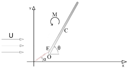
Figure 1: Cross-sectional sketch of the flapping device. $C$ denotes the wing center of mass, $O$ is the wing leading edge and $E$ is the anchor point of the elastic spring (supposed to have a zero rest length). The oriented curved arrows fix the convention on the positiveness of angles and moments. The angle $\alpha$ is magnified for the sake of clarity, the analysis being mostly in the linear regime where the wing is almost aligned along the unperturbed flow.

the expression for ${\bf F}^{e}$ reads:

$$F^{e}_{x}=-k\,x_{C}$$ (1)

$$F^{e}_{y}=-k\,(y_{C}-r\,L\,\theta)\;\;\;,$$ (2)

where lowercase coordinates indicate perturbations with respect to the equilibrium configuration and $k$ is the spring constant.
The resulting equations of motion for the perturbations are:

$$m\,\ddot{x}_{C} = -k\,x_{C}$$ (3)

$$m\,\ddot{y}_{C} = -k\,(y_{C}-r\,L\,\theta)-F^{L}$$ (4)

$$I_{C}\ddot{\theta} = -(r\,L)^{2}\,k\,\theta+r\,L\,k\,y_{C}+r\,L\,F^{L}+M^{L}_{E}$$ (5)

where $I_{C}$ is the moment of inertia (around the center of mass axis), $m$ is the wing mass, $F^{L}$ and $M^{L}_{E}$ are the lift force and the lift momentum.

2.2 Aerodynamics forces and moments

The expression for $F^{L}$ and $M^{L}_{E}$ can be obtained by treating the point $E$ as one does for the flexural point in the classical ‘pitch-and-plunge’ system (Hodges & Pierce, 2002) and then exploiting Theodorsen’s theory (Bisplinghoff et al., 1957). Because of the fact that the latter assumes a sinusoidal response of the system (with no damping and no amplification), it is fully justified to determine marginal curves in the parameter space separating stable regimes from unstable ones (i.e. the so-called flutter condition). Determining such curves is one of the main aim of the present paper.
According to Theodorsen’s theory, the following expressions arise for $F^{L}$ and $M^{L}_{E}$ (Bisplinghoff et al., 1957):

$$F_{L}=\rho\pi b^{2}\left[\ddot{y}_{E}+X_{L/2}\,\ddot{\theta}\right]+\rho\pi b^{2}U\dot{\theta}+\rho U^{2}L\pi\left[\theta+\frac{\dot{y}_{E}}{U}+X_{3L/4}\,\frac{\dot{\theta}}{U}\right]\,{\cal C}(q)$$ (6)

$$M^{L}_{E} = -\rho U^{2}L\pi X_{L/4}\,\left[\theta+\frac{\dot{y}_{E}}{U}+X_{3L/4}\frac{\dot{\theta}}{U}\right]\,{\cal C}(q)$$ (7)

$$- \rho\pi b^{2}\,X_{L/2}\,\left[\ddot{y}_{E}+X_{L/2}\,\ddot{\theta}\right]-\frac{\rho\pi b^{4}}{8}\ddot{\theta}-X_{3L/4}\,\rho\pi b^{2}U\dot{\theta}$$

where $b\equiv L/2$, and $X_{L/4}$, $X_{L/2}$, and $X_{3L/4}$ are the distances of wing points at $L/4$, $L/2$ and $3L/4$ from the leading edge. All terms involving $b$ are the so-called added-mass terms.
The function ${\cal C}(q)$ is the Theodorsen’s function through which the wake effect on the wing motion can be explicitly taken into account (Bisplinghoff et al., 1957). It depends on the reduced frequency $q\equiv\omega\,L/(2U)$, where $\omega$ is the pulsation associated to the system harmonic response. The form of ${\cal C}(q)$ can be given in terms of Hankel functions (Gradshteyn & Ryzhik, 1980) as:

$${\cal C}(q)=\frac{H_{1}^{(2)}(q)}{H_{1}^{(2)}(q)+i\,H_{0}^{(2)}(q)}\;\;\;.$$ (8)

Eqs. (3)-(5) with the expressions for the aerodynamics force and moment (6) and (7) and the relationships $x_{C}=x_{E}$, $y_{C}=y_{E}+r\,L\theta$ constitute our equations of motion for $x_{C}$, $y_{C}$ and $\theta$ under the constraint of harmonic behavior, as dictated by Theodorsen’s theory.
Some comments on the structure of the equations above are worth discussing. The equation for $x_{C}$ is decoupled from the others; this variable can be thus ignored. With respect to the classical ‘pitch-and-plunge’ problem (Hodges & Pierce, 2002) here $y_{C}$ and $\theta$ are two-way coupled in a stronger way, a consequence of the elastic force acting on the wing which jointly depends on both $y_{C}$ and $\theta$. This is expected to cause interesting and peculiar behaviors.

3 Linear stability analysis

Let us now investigate the normal mode linear stability analysis of the system. This can be easily done by normal mode decomposition:

$$y_{C}(t)=Y\,e^{i\,\omega\,t}+c.c\qquad\theta(t)=\Theta\,e^{i\,\omega\,t}+c.c.\;\;\;,$$

where $c.c.$ stands for complex conjugate.
Plugging the expressions above into Eqs. (4) and (5) we obtain an algebraic linear system for the two (complex) amplitudes $Y$ and $\Theta$. The condition of having nontrivial solutions provides a set of two real equations for the real and immaginary parts of $\omega$. Focusing on the determination of marginal curves associated to flutter conditions, and thus assuming the imaginary part of $\omega$ to be zero, one of the two equations furnishes the relationship between parameters identifying the marginal curve, e.g, $\rho$ as a function of $k$ and $r$.
Due to the presence of Theodorsen’s function the determination of the marginal curve requires the exploitation of standard searching methods to find zeros of the associated (non polynomial) set of equations. This is however a task which can be easily achieved by means of a classical Raphson–Newton method.

As customary, it is convenient to pass to a dimensionless form of all variables. For this purpose, let us define the following dimensionless quantities:

$$t\,\frac{U}{L}\mapsto t\qquad\frac{y_{C}}{L}\mapsto y\qquad\frac{k}{\rho\,U^{2}}\mapsto k\qquad\frac{\rho_{w}\,\delta}{\rho\,L}\mapsto\rho_{w}\;\;\;,$$ (9)

so that the reduced frequency is simply $q=\omega/2$. To define the dimensionless parameters above, we have defined by $\rho$ the fluid density and written the wing mass $m$ as $m=\rho_{w}\delta\,L$, $\rho_{w}$ being the wing density.
The behavior of the marginal curve for $r=0.5$ and $r=0.26$ is reported in Fig. 2. Circles refer to points analyzed by DNS for Re=10000 and Re=60000. Their discussion is postponed to Sec. 4.2.

Figure 2: The marginal curve for $r=0.5$ (left, corresponding to the leading edge anchor point) and $r=0.26$ (right). Circles refer to points analyzed through DNS. For filled circles DNS predict unstable motion; for open circles they predict stability. For comparison, dotted lines represent the marginal curve under the quasi-steady hypothesis. To emphasize variations along the vertical axis, a log scale is used for $\rho_{w}$ .

Dotted lines represent the marginal curves under the quasi-steady hypothesis (i.e. when ${\cal C}(q)=1$ and the equations defining marginal curves are polynomials). This corresponds to neglecting the effect of the wake on the motion of the wing. Some points are worth discussing. The first is on the shape of the marginal curves obtained. They are quite structured and the relationship between the dimensionless parameters associated to the fluttering condition is far from being trivial. The pronounced ‘nose’ for $r=0.5$ around $\rho_{w}\sim 10$, $1/k\sim 0.2$ is an example. This peculiar shape leads to interesting consequence on the fluttering condition in terms, e.g., of the wing mass: there are indeed three different values for the wing mass (actually for the dimensionless quantity $\rho_{w}\,\delta/(\rho\,L)$) leading to fluttering for a fixed spring constant (actually for a fixed dimensionless parameter $k/(\rho U^{2})$). It turns out that, for all spring constants and wind speed, it is impossible to sustain flapping if $\rho_{w}\,\delta/(\rho\,L)<0.59$. The latter threshold has been determined by the quasi-steady assumption that tends to coincide (see dotted line in Fig. 2) with Theodorsen’s marginal curve for small spring constants. On the other hand, for very large value of $\rho_{w}\,\delta/(\rho\,L)$ (order of $300$ for $r=0.5$; a much larger value for $r=0.26$) fluttering is expected at all velocities.
Interestingly, the conclusions above are very sensitive to the value of $r$, i.e., to the relative distance between the wing center of mass and the anchor point (see right frame of Fig. 2).

To better understand the sensitivity to $r$ we report in Fig. 3 the marginal curves in the plane $\rho_{w}$-$r$ for two fixed values of $k$. The non-trivial role played by the couple $\rho_{w}$-$r$ in the emergence of stable/unstable regimes can be clearly detected from the figure.

Figure 3: The marginal curve for $k=1/0.2$ (left) and $k=1/0.17$ (right) in the $\rho_{w}$-$r$ space. ‘$U_{1}$’ and ‘$U_{2}$’ denote Unstable regions with one and two unstable normal modes, respectively; ‘S’ stands for Stable. For filled circles DNS predict unstable motion; for open circles they predict stability.

4 Direct numerical simulations

The aim of this section is to give a brief description of the numerical method used to numerically approximate the laminar incompressible Navier–Stokes equations (so in essence we are doing direct numerical simulations or DNS) and verify the predictions obtained from the normal mode linear stability analysis with the solutions obtained from the DNS simulations.
It is beyond the scope of the present paper to fully analyze the shape and position of the obtained marginal curves in the whole parameter space $k$-$\rho_{w}$. This issue is indeed quite expensive from the numerical viewpoint and it will be eventually postponed to a possible future analysis. Rather, our aim is to corroborate our former, and to some extent surprising, conclusions on the nontrivial shape of the marginal curves.

4.1 The numerical method

Hereupon, we briefly outline the solution methodology used to solve the governing equations on moving overlapping structured grids. The complete description of the numerical method and gridding methodology can be found in the papers by Henshaw (1994) and Chesshire & Henshaw (1990).
In this manuscript, we numerically approximate the laminar incompressible Navier–Stokes equations by using the velocity-pressure formulation or pressure-Poisson equation (PPE) (Henshaw, 1994; Sani et al., 2006; Petersson, 2001; Gresho, 1991).

$$\frac{\partial\textbf{u}}{\partial t}+\textbf{u}\cdot\bm{\partial}\textbf{u}=-\frac{\bm{\partial}p}{\rho}+\nu\partial^{2}\textbf{u}\quad \textit{for}\quad\textbf{x}\in\mathcal{D},\quad t>0,$$ (10)

$${\frac{\partial^{2}p}{\rho}}+\partial_{\alpha}\textbf{u}\cdot\bm{\partial}u_{\alpha}=0\quad \textit{for}\quad\textbf{x}\in\mathcal{D},\quad t>0,$$ (11)

with the following boundary and initial conditions

$$B\left(\textbf{u},p\right) =0\qquad\qquad\qquad \textit{for}\quad\textbf{x}\in\partial\mathcal{D},\quad\,\,\,t>0,$$ (12)

$$\bm{\partial}\cdot\textbf{u} =0\qquad\qquad\qquad \textit{for}\quad\textbf{x}\in\partial\mathcal{D},\quad\,\,\,t>0,$$ (13)

$$\textbf{u}\left(\textbf{x},0\right) =\textbf{u}_{0}\left(\textbf{x}\right)\qquad\qquad\quad\,\, \textit{for}\quad\textbf{x}\in\mathcal{D}.$$ (14)

In this initial-boundary-value problem (IBVP), $\textbf{x}=(x,y)$ (for $\mathbb{N}=2$ where $\mathbb{N}$ is the number of space dimensions) is the physical space coordinates, $\mathcal{D}$ is a bounded domain in $\Re^{\mathbb{N}}$, $\partial\mathcal{D}$ is the boundary of the domain $\mathcal{D}$, $t$ is the physical time, $\textbf{u}=(u,v)$ is the velocity field, $p$ is the pressure, $\nu$ is the kinematic viscosity, $\rho$ is the density, $B$ is a boundary operator initial data.
and $\textbf{u}_{0}$ are the initial conditions. Hence, we look for an approximate numerical solution of equations (10) and (11) in a given domain $\mathcal{D}$, with prescribed boundary conditions and given initial conditions (equations (12)-(14)). Equations (10)-(14) are solved in logically rectangular grids in the transformed computational space $\mathcal{C}=\mathcal{C}(\xi,\eta,t)$ (refer to Chesshire & Henshaw (1990); Drikakis & Rider (2004); Guerrero (2009, 2010); Henshaw (1994); Vinokur (1974) for a detailed derivation), using second-order centred finite-difference approximations on structured overlapping grids.
In general, the motion of the component grids $\mathcal{G}_{g}$ of an overlapping grid system $\mathbb{G}=\{\mathcal{G}_{g}\}$, may be an user-defined time dependent function, may obey the Newton-Euler equations for the case of rigid body motion or may correspond to the boundary nodes displacement in response to the forces exerted by the fluid pressure for the case of fluid-structure interaction problems. For moving overlapping grids, Eqs.  (10)-(11) are expressed in a reference frame moving with the component grid as follows,

$$\frac{\partial\textbf{u}}{\partial t}+\left[\left(\textbf{u}-\dot{\textbf{G}}\right)\cdot\bm{\partial}\right]\textbf{u}=-\frac{\bm{\partial}p}{\rho}+\nu\partial^{2}\textbf{u}\quad \mbox{for}\quad\textbf{x}\in\mathcal{D},\quad t>0,$$ (15)

$${\frac{\partial^{2}p}{\rho}}+\partial_{\alpha}\textbf{u}\cdot\bm{\partial}u_{\alpha}=0\quad \mbox{for}\quad\textbf{x}\in\mathcal{D},\quad t>0,$$ (16)

where $\dot{\textbf{G}}$ is the rate of change of the position of a given set of grid points $\textbf{x}_{p}^{g}$ of a component grid $\mathcal{G}_{g}$ in the physical space (grid velocity). It is important to mention that the new governing equations expressed in the moving reference frame must be accompanied by proper boundary conditions. For a moving body with a corresponding moving no-slip wall, only one constraint may be applied and this corresponds to the velocity on the wall, such as

$$\textbf{u}\left(\textbf{x}_{p}^{g}|_{wall},t\right)=\dot{\textbf{G}}\left(\textbf{x}_{p}^{g}|_{wall},t\right),\quad\mbox{where}\quad\textbf{x}_{p}^{g}|_{wall}\in\partial\mathcal{D}_{wall}\left(t\right).$$ (17)

Finally, in order to keep the solution of the pressure equation decoupled from the solution of the velocity components, we choose a time stepping scheme for the velocity components that only involves the pressure from the previous time steps (split-step scheme) (Henshaw, 1994; Henshaw & Petersson, 2003). Then, the discretized equations are integrated in time using a semi-implicit multi-step method, that uses a Crank-Nicolson scheme for the viscous terms and a second-order Adams-Bashforth/Adams-Moulton predictor-corrector approach for the convective terms and pressure. This solution method yields a stable second-order accurate in space and time numerical scheme on moving overlapping structured grids.
To assemble the overlapping grid system $\mathbb{G}$ and solve the laminar incompressible Navier-Stokes equations in their velocity-pressure formulation, the Overture framework is used. The large sparse non-linear system of equations arising from the discretization of the laminar incompressible Navier-Stokes equations is solved using the PETSc library, which was interfaced with Overture. The system of non-linear equations is then solved using a Newton-Krylov iterative method, in combination with a suitable preconditioner.

As a final remark, for the range of Reynolds numbers considered in this study, no turbulence model or sub-grid scale model is used for the numerical simulations conducted, so in essence two-dimensional direct-numerical simulations (DNS) are performed. Despite the fact that the grid does not resolve the smallest scales in the far-wake region (where small scale activity is however strongly reduced), the grid resolution is always more than adequate. It is so also in the near-wake flow field where the resolution is sufficiently high to properly resolve the small scales so that accurate instantaneous drag and lift forces are computed.

4.2 Numerical settings and results

We confine our attention to the marginal curve of Fig. 2 (left), performing direct numerical simulations for different values of $(\rho_{w}$, $1/k)$, for Reynolds numbers between $10000$ and $60000$. We almost never place ourselves too close to the predicted marginal line to avoid a very slow increase/decrease of the initial perturbation and thus to avoid long and expensive simulations. As far as initial perturbations are concerned, we firstly consider the one dimensional problem (along $x$) and we reach the equilibrium position under that condition. At this stage we impose a perturbation on the angle $\theta$, of the order of $10^{-5}\,deg$, and leave the system free to evolve.

Figure 4: Time behavior of the pitching angle $\theta$ (deg), on the left, and of the $y$-coordinate of the wing leading edge, on the right, for the unstable case with $1/k=0.35$ and $\rho_{w}=3.5$ and $r=1/2$. All variables are made dimensionless by (9).

Figure 5: The same as in Fig. 4 but for the stable case $1/k=0.1$ and $\rho_{w}=20$.

Filled circles in Fig. 2 (left) are associated to unstable behavior; stability is represented by open circles. The agreement with our predictions based on Theodorsen’s theory is good.
Typical time behavior for the angle $\theta$ and the leading edge vertical coordinate $y_{O}$ are reported in Fig. 4 for $\rho_{w}=3.5$ and $1/k=0.35$ (unstable case, see also the movie) and in Fig. 5 for $\rho_{w}=20$ and $1/k=0.1$ (stable case, see also the movie). Notice how the unstable case reaches a fully nonlinear stage characterized by a sustained flapping with a $y$ excursion of the wing leading edge of order one (with lengths normalized by the wing chord). This is a very promising result in view of applications related to the energy harvesting where elastomeric capacitors need to be stretched/compressed much, in order to produce reasonable amounts of electric energy.
The example shown in Fig. 4 tells us that an infinitesimal perturbation yields the system to a finite-amplitude limit cycle associated to unceasing flapping. A natural question which arises is on whether unceasing flapping can be observed if a finite size perturbation is applied to configurations which are stable with respect to small perturbations. As an example we address this question for the couple of parameters $\rho_{w}=20$ and $1/k=0.1$. The initial angle $\theta$ is now $90\ deg$. The resulting time behaviors for $\theta$ and $y_{O}$ are reported in Fig. 6. We do not detect any tendency of relaxation toward the aligned configuration, a fingerprint of a subcritical instability.

Figure 6: Time behavior of the pitching angle $\theta$ (deg), on the left, and of the $y$-coordinate of the wing leading edge, on the right, for the linearly stable case with $1/k=0.1$, $\rho_{w}=20$ and $r=1/2$. All variables are made dimensionless by (9). The initial perturbation is here of finite size.

5 Conclusions

A simple flapping system has been presented and investigated both analytically and numerically. Three dimensionless parameters come into play and their role on the resulting flapping states appear to be highly non trivial. This property has been confirmed by numerical simulations we carried out in the range of Reynolds numbers between $10000$ and $60000$.
Both supercritical instabilities and subcritical instabilities have been found in our system.

Our findings have direct applicability to the energy harvesting problem by fluid-structure interaction (Boragno et al., 2012). We have found sets of parameters leading to unceasing flapping for which the excursion of the leading edge is of the same order of the wing chord. Once our spring is replaced by an elastomeric capacitor, the observed large amplitude of the wing oscillations is a necessary condition for extracting a reasonable amount of energy from the device.

We thank Alessandro Bottaro and Jan Oscar Pralits for many useful discussions and suggestions. The use of the computing resources at CASPUR high-performance computing center was possible thanks to the HPC Grant 2011. The use of the computing facilities at the high-performance computing center of the University of Stuttgart was possible thanks to the support of the HPC-Europa2 project (project number 238398), with the support of the European Community – Research Infrastructure Action of the FP7.

References

- Aulisa et al. (2006) Aulisa, E., Manservisi, S. & Seshaiyer, P. 2006 A computational multilevel approach for solving 2d Navier–Stokes equations over non-matching grids. Computer Methods in Applied Mechanics and Engineering 195, 4604–4616.
- Bisplinghoff et al. (1957) Bisplinghoff, R.L., Ashley, H. & Halfman, R.L. 1957 Aeroelasticity. Addison-Wesley.
- Boragno et al. (2012) Boragno, C., Festa, R. & Mazzino, A. 2012 Wind induced oscillations of an elastically bounded flapping wing. Submitted to Nature Physics .
- Chesshire & Henshaw (1990) Chesshire, G. & Henshaw, W. 1990 Composite overlapping meshes for the solution of partial differential equations. Journal of Computational Physics 90, 1–64.
- Dowell & Kenneth (2001) Dowell, E.H. & Kenneth, C.H. 2001 Modeling of fluid-structure interaction. Annual Review of Fluid Mechanics 33, 445–490.
- Drikakis & Rider (2004) Drikakis, D. & Rider, W. 2004 High-Resolution Methods for Incompressible and Low-Speed Flows. Springer.
- Favier et al. (2009) Favier, J., Dauptain, A., Basso, D. & Bottaro, A. 2009 Passive separation control using a self-adaptive hairy coating. Journal of Fluid Mechanics 627, 451–483.
- Fish & Lauder (2006) Fish, F.E. & Lauder, G.V. 2006 Passive and active flow control by swimming fishes and mammals. Annual Review of Fluid Mechanics 38, 193–224.
- Gradshteyn & Ryzhik (1980) Gradshteyn, I.S. & Ryzhik, I.M. 1980 Table of Integrals, Series and Products. Academic Press.
- Gresho (1991) Gresho, P.M. 1991 Incompressible fluid dynamics: some fundamental formulation issues. Annual Review of Fluid Mechanics 23, 413–453.
- Guerrero (2009) Guerrero, J. 2009 Numerical simulation of the unsteady aerodynamics of flapping flight. PhD thesis, University of Genoa. Deparment of Civil, Enviromental and Architectural Engineering, Italy.
- Guerrero (2010) Guerrero, J. 2010 Wake signature and Strouhal number dependence of finite-span flapping wings. Journal of Bionic Engineering 7, S109–S122.
- Henshaw (1994) Henshaw, W.D. 1994 A fourth-order accurate method for the incompressible Navier–Stokes equations on overlapping grids. Journal of Computational Physics 113, 13–25.
- Henshaw & Petersson (2003) Henshaw, W. & Petersson, N. 2003 A split-step scheme for the incompressible Navier–Stokes equations. In Numerical Solutions of Incompressible Flows. M.M. Hafez (ed.), World Scientific Publishing Co. Singapore.
- Hodges & Pierce (2002) Hodges, D.H. & Pierce, G.A 2002 Introduction to Structural Dynamics and Aeroelasticity. Cambridge University Press.
- McKinney & DeLaurier (1981) McKinney, W. & DeLaurier, J. 1981 The wingmill: An oscillating-wing windmill. Journal of Energy 5, 109–115.
- Petersson (2001) Petersson, N. 2001 Stability of pressure boundary conditions for stokes and Navier–Stokes equations. Journal of Computational Physics 172, 40–70.
- Sane (2003) Sane, S. P. 2003 The aerodynamics of insect flight. The Journal of Experimental Biology 206, 4191–4208.
- Sani et al. (2006) Sani, R.L., Shen, J., Pironneau, O. & Gresho, P.M. 2006 Pressure boundary condition for the time-dependent incompressible Navier–Stokes equations. International Journal for Numerical Methods in Fluids 50, 673–682.
- de Tullio et al. (2009) de Tullio, M.D., Cristallo, A., Balaras, E. & Verzicco, R. 2009 Direct numerical simulation of the pulsatile flow through an aortic bileaflet mechanical heart valve. Journal of Fluid Mechanics 622, 259–290.
- Vinokur (1974) Vinokur, M. 1974 Conservation equations of gas-dynamics in curvilinear coordinate systems. Journal of Computational Physics 14, 105–125.