Robust constraints on dark energy and gravity
from galaxy clustering data

Abstract

Galaxy clustering data provide a powerful probe of dark energy. We examine how the constraints on the scaled expansion history of the universe, $x_{h}(z)=H(z)s$ (with $s$ denoting the sound horizon at the drag epoch), and the scaled angular diameter distance, $x_{d}(z)=D_{A}(z)/s$, depend on the methods used to analyze the galaxy clustering data. We find that using the observed galaxy power spectrum, $P_{g}^{obs}(k)$, $x_{h}(z)$ and $x_{d}(z)$ are measured more accurately and are significantly less correlated with each other, compared to using only the information from the baryon acoustic oscillations (BAO) in $P_{g}^{obs}(k)$. Using the $\{x_{h}(z),x_{d}(z)\}$ from $P_{g}^{obs}(k)$ gives a DETF dark energy FoM approximately a factor of two larger than using the $\{x_{h}(z),x_{d}(z)\}$ from BAO only; this provides a robust conservative method to go beyond BAO only in extracting dark energy information from galaxy clustering data.

We find that a Stage IV galaxy redshift survey, with $0.7<z<2$ over 15,000 (deg)², can measure $\{x_{h}(z),x_{d}(z),f_{g}(z)G(z)\tilde{P}_{0}^{1/2}/s^{4}\}$ with high precision (where $f_{g}(z)$ and $G(z)$ are the linear growth rate and factor of large scale structure respectively, and $\tilde{P}_{0}$ is the dimensionless normalization of $P_{g}^{obs}(k)$), when redshift-space distortion information is included. The measurement of $f_{g}(z)G(z)\tilde{P}_{0}^{1/2}/s^{4}$ provides a powerful test of gravity, and significantly boosts the dark energy FoM when general relativity is assumed.

1 Introduction

The cosmic acceleration (i.e., dark energy) was discovered in 1998 (Riess et al., 1998; Perlmutter et al., 1999), and we are still in the dark about the nature of this mystery. We can hope to measure both the cosmic expansion history and the cosmic large scale structure growth history accurately and precisely with galaxy clustering (see, e.g., Guzzo et al. (2008); Wang (2008a)) and weak lensing (see, e.g., Knox, Song, & Tyson (2006); Zhang et al. (2007); Heavens (2009)) data from a space mission such as Euclid (Laureijs et al., 2011), and differentiate the two possible explanations for the observed cosmic acceleration: a new energy component, or a modification of Einstein’s theory of gravity.

Galaxy clustering has long been used as a cosmological probe (see, e.g., Hamilton (1998)). At present, the largest data set comes from the SDSS III Baryon Oscillation Spectroscopic Survey (BOSS), see Anderson et al. (2012) and Reid et al. (2012).

Here we explore different analysis techniques for galaxy clustering data, in order to obtain robust constraints on dark energy and general relativity. It is important to study how the dark energy and gravity constraints depend on the assumptions we make about the information that can be extracted from galaxy redshift survey data.

We present our methods in Sec.2, results in Sec.3, and summarize in Sec.4.

2 Methodology

2.1 The Fisher Matrix Formalism

We use the Fisher matrix formalism to study the parameter estimation using galaxy clustering data (Tegmark, 1997; Seo & Eisenstein, 2003), based on the approach developed in Wang (2006, 2008a, 2010a); Wang et al. (2010). In the limit where the length scale corresponding to the survey volume is much larger than the scale of any features in the observed galaxy power spectrum $P_{g}(k)$, we can assume that the likelihood function for the band powers of a galaxy redshift survey is Gaussian (Feldman, Kaiser, & Peacock, 1994), with a measurement error in $\ln P(\mbox{\bf k})$ that is proportional to $[V_{eff}(\mbox{\bf k})]^{-1/2}$, with the effective volume of the survey defined as

$$V_{eff}(k,\mu) \equiv \int d\mbox{\bf r}^{3}\left[\frac{n(\mbox{\bf r})P_{g}(k,\mu)}{n(\mbox{\bf r})P_{g}(k,\mu)+1}\right]^{2}$$ (1)

$$= \left[\frac{nP_{g}(k,\mu)}{nP_{g}(k,\mu)+1}\right]^{2}V_{survey},$$

where the comoving number density $n$ is assumed to only depend on the redshift (and constant in each redshift slice) for simplicity in the last part of the equation.

In order to propagate the measurement error in $\ln P_{g}(\mbox{\bf k})$ into measurement errors for the parameters $p_{i}$, we use the Fisher matrix (Tegmark, 1997)

$$F_{ij}=\int_{k_{min}}^{k_{max}}\frac{\partial\ln P_{g}(\mbox{\bf k})}{\partial p_{i}}\frac{\partial\ln P_{g}(\mbox{\bf k})}{\partial p_{j}}\,V_{eff}(\mbox{\bf k})\,\frac{d\mbox{\bf k}^{3}}{2\,(2\pi)^{3}}$$ (2)

where $p_{i}$ are the parameters to be estimated from data, and the derivatives are evaluated at parameter values of the fiducial model. Note that the Fisher matrix $F_{ij}$ is the inverse of the covariance matrix of the parameters $p_{i}$ if the $p_{i}$ are Gaussian distributed.

The observed galaxy power spectrum can be reconstructed using a particular reference cosmology, including the effects of bias and redshift-space distortions (Seo & Eisenstein, 2003):

$$P_{g}^{obs}(k^{ref}_{\perp},k^{ref}_{\parallel}) = \frac{\left[D_{A}(z)^{ref}\right]^{2}H(z)}{\left[D_{A}(z)\right]^{2}H(z)^{ref}}\,b^{2}\left(1+\beta\,\mu^{2}\right)^{2}\cdot$$ (3)

$$\,\,\,\cdot[G(z)]^{2}P_{m}(k)_{z=0}+P_{shot},$$

where $H(z)=\dot{a}/{a}$ (with $a$ denoting the cosmic scale factor) is the Hubble parameter, and $D_{A}(z)=r(z)/(1+z)$ is the angular diameter distance at $z$, with the comoving distance $r(z)$ given by

$$r(z)=c\,|\Omega_{k}|^{-1/2}{\rm sinn}\left[|\Omega_{k}|^{1/2}\,\int_{0}^{z}\frac{dz^{\prime}}{H(z^{\prime})}\right],$$ (4)

where ${\rm sinn}(x)=\sin(x)$, $x$, $\sinh(x)$ for $\Omega_{k}<0$, $\Omega_{k}=0$, and $\Omega_{k}>0$ respectively. The bias between galaxy and matter distributions is denoted by $b(z)$. The linear redshift-space distortion parameter $\beta(z)=f_{g}(z)/b(z)$ (Kaiser, 1987), where $f_{g}(z)$ is the linear growth rate; it is related to the linear growth factor $G(z)$ (normalized such that $G(0)=1$) as follows

$$f_{g}(z)=\frac{\mbox{d}\ln G(z)}{\mbox{d}\ln a}.$$ (5)

Note that $\mu=\mbox{\bf k}\cdot\hat{\mbox{\bf r}}/k$, with $\hat{\mbox{\bf r}}$ denoting the unit vector along the line of sight; k is the wavevector with $|\mbox{\bf k}|=k$. Hence $\mu^{2}=k^{2}_{\parallel}/k^{2}=k^{2}_{\parallel}/(k^{2}_{\perp}+k^{2}_{\parallel})$, where

$$k_{\parallel} = \mbox{\bf k}\cdot\hat{\mbox{\bf r}}=k\mu$$

$$k_{\perp} = \sqrt{k^{2}-k^{2}_{\parallel}}=k\sqrt{1-\mu^{2}}.$$ (6)

The values in the reference cosmology are denoted by the subscript “ref”, while those in the true cosmology have no subscript. Note that

$$k^{ref}_{\perp}=k_{\perp}D_{A}(z)/D_{A}(z)^{ref},\hskip 14.22636ptk^{ref}_{\parallel}=k_{\parallel}H(z)^{ref}/H(z).$$ (7)

Eq.(3) characterizes the dependence of the observed galaxy power spectrum on $H(z)$ and $D_{A}(z)$ due to BAO, as well as the sensitivity of a galaxy redshift survey to the linear redshift-space distortion parameter $\beta$ (Kaiser, 1987). The linear matter power spectrum at $z=0$ is given by

$$P_{m}(k)_{z=0}=P_{0}\,k^{n_{s}}T^{2}(k),$$ (8)

where $T(k)$ denotes the matter transfer function.

The measurement of $f_{g}(z)$ given $\beta(z)=f_{g}(z)/b(z)$ requires an additional measurement of the bias $b(z)$, which could be obtained from the galaxy bispectrum (Matarrese, Verde, & Heavens, 1997; Verde et al., 2002). Alternatively, we can rewrite Eq.(3) as

$$\overline{P_{g}^{obs}(k^{ref}_{\perp},k^{ref}_{\parallel})}$$

$$\equiv P_{g}^{obs}(k^{ref}_{\perp},k^{ref}_{\parallel})/(h^{-1}\mbox{Mpc})^{3}$$

$$= \frac{\left[D_{A}(z)^{ref}\right]^{2}H(z)}{\left[D_{A}(z)\right]^{2}H(z)^{ref}}\left(\frac{k}{\mbox{Mpc}^{-1}}\right)^{n_{s}}T^{2}(k)\cdot$$

$$\cdot\left[\sigma_{g}(z)+f_{g}(z)\sigma_{m}(z)\,\mu^{2}\right]^{2}+P_{shot},$$

where we have defined

$$\sigma_{g}(z) \equiv b(z)\,G(z)\,\tilde{P}_{0}^{1/2}$$

$$\sigma_{m}(z) \equiv G(z)\,\tilde{P}_{0}^{1/2},$$ (10)

The dimensionless power spectrum normalization constant $\tilde{P}_{0}$ is just $P_{0}$ in Eq.(8) in appropriate units:

$$\tilde{P}_{0}\equiv\frac{P_{0}}{(\mbox{Mpc}/h)^{3}(\mbox{Mpc})^{n_{s}}}=\frac{\sigma_{8}^{2}}{I_{0}\,h^{n_{s}}},$$ (11)

The second part of Eq.(11) is relevant if $\sigma_{8}$ is used to normalize the power spectrum. Note that

$$I_{0}\equiv\int_{0}^{\infty}{\rm d}\bar{k}\,\frac{\bar{k}^{n_{s}+2}}{2\pi^{2}}\,T^{2}(\bar{k}\cdot h\mbox{Mpc}^{-1})\,\left[\frac{3j_{1}(8\bar{k})}{8\bar{k}}\right]^{2},$$ (12)

where $\bar{k}\equiv k/[h\,\mbox{Mpc}^{-1}]$, and $j_{1}(kr)$ is spherical Bessel function. Note that $I_{0}=I_{0}(\omega_{m},\omega_{b},n_{s},h)$. Since $k_{\parallel}$ and $k_{\perp}$ scale as $H(z)$ and $1/D_{A}(z)$ respectively, $\overline{P_{g}^{obs}(k)}$ in Eq.(2.1) does not depend on $h$.

Eq.(2.1) is analogous to the approach of Song & Percival (2009), who proposed the use of $f_{g}(z)\sigma_{8}(z)$ to probe growth of large scale structure. The difference is that Eq.(2.1) uses $f_{g}(z)\sigma_{m}(z)\equiv f_{g}(z)G(z)\tilde{P}_{0}^{1/2}$, which does not introduce an explicit dependence on $h$ (as in the case of using $f_{g}(z)\sigma_{8}(z)$).

The uncertainty in redshift measurements is included by multiplying $P_{g}(k)$ with the damping factor, $e^{-k^{2}\mu^{2}\sigma_{r}^{2}}$, due to redshift uncertainties, with

$$\sigma_{r}=\frac{\partial r}{\partial z}\,\sigma_{z}$$ (13)

where $r$ is the comoving distance. Note that the damping factor should be held constant when taking derivatives of $P_{g}(k)$.

2.2 $P(k)$ Method

Including the nonlinear effects explicitly, we can write (Seo & Eisenstein, 2007)

$$\frac{\partial P_{g}(k,\mu|z)}{\partial p_{i}}=\frac{\partial P_{g}^{lin}(k,\mu|z)}{\partial p_{i}}\cdot\exp\left(-\frac{1}{2}\,k^{2}\Sigma_{nl}^{2}\right).$$ (14)

The damping is applied to derivatives of $P_{g}(k)$, rather than $P_{g}(k)$, to ensure that no information is extracted from the damping itself. Eq.(2) becomes

$$F_{ij} = V_{survey}\int_{-1}^{1}d\mu\int_{k_{min}}^{k_{max}}\frac{\partial\ln P_{g}^{lin}(k,\mu)}{\partial p_{i}}\frac{\partial\ln P_{g}^{lin}(k,\mu)}{\partial p_{j}}\,\cdot$$ (15)

$$\cdot\left[\frac{nP_{g}^{lin}(k,\mu)}{nP_{g}^{lin}(k,\mu)+1}\right]^{2}\,e^{-k^{2}\Sigma_{nl}^{2}}\,\frac{2\pi k^{2}dk}{2\,(2\pi)^{3}}.$$

The linear galaxy power spectrum $P_{g}^{lin}(k,\mu|z)$ is given by Eq.(2.1). The nonlinear damping scale

$$\Sigma_{nl}^{2} = (1-\mu^{2})\Sigma_{\perp}^{2}+\mu^{2}\Sigma^{2}_{\parallel}$$

$$\Sigma_{\parallel} = \Sigma_{\perp}(1+f_{g})$$

$$\Sigma_{\perp} = 12.4\,h^{-1}{\rm Mpc}\,\left(\frac{\sigma_{8}}{0.9}\right)\cdot 0.758\,G(z)\,p_{NL}$$ (16)

$$= 8.355\,h^{-1}{\rm Mpc}\,\left(\frac{\sigma_{8}}{0.8}\right)\cdot G(z)\,p_{NL}.$$

The parameter $p_{NL}$ indicates the remaining level of nonlinearity in the data; with $p_{NL}=0.5$ (50% nonlinearity) as the best case, and $p_{NL}=1$ (100% nonlinearity) as the worst case (Seo & Eisenstein, 2007). For a fiducial model based on WMAP3 results (Spergel et al., 2007) ($\Omega_{m}=0.24$, $h=0.73$, $\Omega_{\Lambda}=0.76$, $\Omega_{k}=0$, $\Omega_{b}h^{2}=0.0223$, $\tau=0.09$, $n_{s}=0.95$, $T/S=0$), $A_{0}=0.5817$, $P_{0.2}=2710\,\sigma_{8,g}^{2}$ (Seo & Eisenstein, 2007).

In the $P(k)$ method, the full set of parameters that describe the observed $P_{g}(k)$ in each redshift slice are: $\{\ln H(z_{i})$, $\ln D_{A}(z_{i})$, $\ln[f_{g}(z_{i})\sigma_{m}(z_{i})]$, $\ln\sigma_{g}(z_{i})$, $P_{shot}^{i}$; $\omega_{m}$, $\omega_{b}$, $n_{s}\}$, where $\omega_{m}\equiv\Omega_{m}h^{2}$, and $\omega_{b}\equiv\Omega_{b}h^{2}$. We marginalize over $\{\ln\sigma_{g}(z_{i}),P_{shot}^{i}\}$ in each redshift slice, to obtain a Fisher matrix for $\{\ln H(z_{i}),\ln D_{A}(z_{i}),\ln[f_{g}(z_{i})\sigma_{m}(z_{i})];\omega_{m},\omega_{b},n_{s}\}$. This full Fisher matrix, or a smaller set marginalized over various parameters, is projected into the standard set of cosmological parameters $\{w_{0},w_{a},\Omega_{X},\Omega_{k},\omega_{m},\omega_{b},n_{s},\ln A_{s}\}$. There are four different ways of utilizing the information from $P(k)$ (see Sec.3.3).

2.3 BAO Only Method

The power of galaxy clustering as a dark energy probe was first recognized via studies of baryon acoustic oscillations (BAO) as a standard ruler (Blake & Glazebrook, 2003; Seo & Eisenstein, 2003). The BAO only method essentially approximates $\partial P_{g}^{lin}(k,\mu)/\partial p_{i}$ with $\partial P_{b}^{lin}(k,\mu|z)/\partial p_{i}$ in the derivatives in Eq.(15), with the power spectrum that contains baryonic features, $P_{b}^{lin}(k,\mu)$, given by (Seo & Eisenstein, 2007)

$$P_{b}^{lin}(k,\mu|z)=\sqrt{8\pi^{2}}A_{0}\,P_{g}^{lin}(k_{0.2},\mu|z)\frac{\sin(x)}{x}\exp\left[-(k\Sigma_{s})^{1.4}\right],$$ (17)

where $P_{g}^{lin}(k,\mu|z)$ is the linear galaxy power spectrum, and the Silk damping scale $\Sigma_{s}=8.38\,h^{-1}{\rm Mpc}$. We have defined

$$k_{0.2} \equiv 0.2\,h\,{\rm Mpc}^{-1}$$ (18)

$$x \equiv \left(k^{2}_{\perp}s^{2}_{\perp}+k^{2}_{\parallel}s^{2}_{\parallel}\right)^{1/2}$$ (19)

Defining

$$p_{1} = \ln s_{\perp}^{-1}=\ln(D_{A}/s)\equiv\ln(x_{h}),$$ (20)

$$p_{2} = \ln s_{\parallel}=\ln(sH)\equiv\ln(x_{d}),$$ (21)

substituting Eq.(17) into Eq.(15), and making the approximation of $\cos^{2}x\sim 1/2$, we find

$$F_{ij}\simeq V_{survey}A_{0}^{2}\int_{0}^{1}{\rm d}\mu\,f_{i}(\mu)\,f_{j}(\mu)\int_{0}^{k_{max}}{\rm d}k\,k^{2}\cdot$$

$$\hskip 1.4457pt\cdot\left[\frac{P^{lin}_{m}(k|z=0)}{P^{lin}_{m}(k_{0.2}|z=0)}+\frac{1}{nP^{lin}_{g}(k_{0.2},\mu|z)\,e^{-k^{2}\mu^{2}\sigma_{r}^{2}}}\right]^{-2}$$

$$\hskip 1.4457pt\cdot\exp\left[-2(k\Sigma_{s})^{1.4}-k^{2}\Sigma_{nl}^{2}\right],$$ (22)

where $P_{g}^{lin}(k_{0.2},\mu|z)$ is given by Eq.(2.1) with $k=k_{0.2}$.

The functions $f_{i}(\mu)$ are given by

$$f_{1}(\mu) = \partial\ln x/\partial p_{1}=\mu^{2}-1$$ (23)

$$f_{2}(\mu) = \partial\ln x/\partial p_{2}=\mu^{2}.$$ (24)

The BAO only method gives $\{x_{h}(z),x_{d}(z)\}$ that are correlated at the level of $\sim$41% with each other, but are uncorrelated for different redshift slices by construction.

2.4 Assumptions and Priors

We use the fiducial model adopted by the FoMSWG (Albrecht et al., 2009), with $\omega_{m}\equiv\Omega_{m}h^{2}=0.1326$, $\omega_{b}\equiv\Omega_{b}h^{2}=0.0227$, $h=0.719$, $\Omega_{k}=0$, $w=-1.0$, $n_{s}=0.963$, and $\sigma_{8}=0.798$. No priors are used in deriving $\{x_{h}(z),x_{d}(z),f_{g}(z)\sigma_{m}(z)/s^{4}\}$, which provide model-independent constraints on the cosmic expansion history and the growth rate of cosmic large scale structure. These allow the detection of dark energy evolution, and the differentiation between an unknown energy component and modified gravity as the causes for the observed cosmic acceleration.

In order to derive dark energy figure of merit (FoM), as defined by the DETF (Albrecht et al., 2006), we project our Fisher matrices into the standard set of dark energy and cosmological parameters: $\{w_{0},w_{a},\Omega_{X},\Omega_{k},\omega_{m},\omega_{b},n_{s},\ln A_{s}\}$. To include Planck priors, we convert the Planck Fisher matrix for 44 parameters (including 36 parameters that parametrize the dark energy equation of state in redshift bins) from the FoMSWG into a Planck Fisher matrix for this set of dark energy and cosmological parameters.

We present all our results for StageIV+BOSS spectroscopic galaxy redshift surveys. The Stage IV galaxy redshift survey is assumed to cover 15,000 (deg)², with H$\alpha$ flux limit of $3\times 10^{-16}$ erg s^-1cm^-2, an efficiency of $e=0.50$, a redshift range of $0.7<z<2.05$, and a redshift accuracy of $\sigma_{z}/(1+z)=0.001$. The galaxy number density is given by Geach et al. (2010), and the galaxy bias function is given by Orsi et al. (2010). This is similar to the baseline of the Euclid galaxy redshift survey (Laureijs et al., 2011). The BOSS survey is assumed to cover 10,000 (deg)², a redshift range of $0.1<z<0.7$, with a fixed galaxy number density of $n=3\times 10^{-4}h^{3}$Mpc^-3, and a fixed linear bias of $b=1.7$.

3 Results

3.1 Measurement of $H(z)$ and $D_{A}(z)$

The $H(z)$ and $D_{A}(z)$ observables that correspond to the BAO scale are

$$x_{h}(z) \equiv H(z)s$$

$$x_{d}(z) \equiv D_{A}(z)/s$$ (25)

where $s$ is the sound horizon scale at the drag epoch (Hu & Sugiyama, 1996).

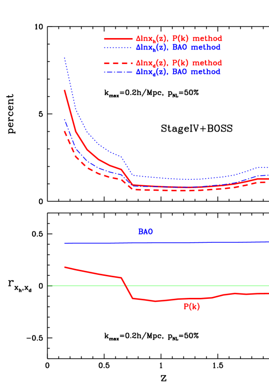
Figure 1: Precision of $x_{h}(z)\equiv H(z)s$ and $x_{d}(z)\equiv D_{A}(z)/s$ expected from StageIV+BOSS. The top panel shows the percentage errors on $x_{h}(z)$ and $x_{d}(z)$ per $\Delta z=0.1$ redshift bin, the bottom panel shows the normalized correlation coefficient between $x_{h}(z)$ and $x_{d}(z)$.

Fig.1 shows the measurement precision of $x_{h}(z)$ and $x_{d}(z)$ for StageIV+BOSS. The top panel shows the percentage errors on $x_{h}(z)$ and $x_{d}(z)$, the bottom panel shows the normalized correlation coefficient between them. The thick solid and dashed lines represent the measurement precision of $x_{h}(z)$ and $x_{d}(z)$ from the $P(k)$ method, marginalized over all other parameters. The thin dotted and dot-dashed lines represent the measurement of $x_{h}(z)$ and $x_{d}(z)$ from the BAO only method.

Note that the $x_{h}(z)$ and $x_{d}(z)$ measured using $P(k)$ are only weakly correlated. Since $x_{h}(z)$ and $x_{d}(z)$ represent independent degrees of freedom in a galaxy redshift survey, they should not be strongly correlated. This is consistent with the findings of Chuang & Wang (2011) from their analysis of SDSS LRG data.

The $x_{h}(z)$ and $x_{d}(z)$ from using the BAO method are correlated with a normalized correlation coefficient of $r\sim 0.41$. They are positively correlated by construction: In both $P(k)$ and BAO only methods, the Fisher matrix element for $\{x_{h}(z),x_{d}(z)\}$ from the same redshift slice is negative. In the $P(k)$ method, the $x_{h}(z)$ and $x_{d}(z)$ from different redshift slices are correlated through the cosmological parameters $\{\omega_{m},\omega_{b},n_{s}\}$ that are measured using information from all the redshift slices. When the cosmological parameters are marginalized over, the dependence on these parameters remain as a weak correlation between $x_{h}(z)$ and $x_{d}(z)$. In the BAO method, the $x_{h}(z)$ and $x_{d}(z)$ from different redshift slices are uncorrelated by construction. Inverting the 2$\times$2 Fisher matrix of $x_{h}(z)$ and $x_{d}(z)$ in each redshift slice leads to positive and significant correlation between $x_{h}(z)$ and $x_{d}(z)$.

Finally, note that in using the $P(k)$ method to forecast dark energy constraints, two different methods have been used to account for nonlinear effects:
(1) Setting $k_{max}=\pi/(2R)$, with $R$ given by requiring that $\sigma^{2}(R)$ is small (e.g., $\sigma^{2}(R)=0.25$), and imposing a uniform upper limit cutoff, e.g., $k_{max}\leq 0.2h/\mbox{Mpc}$. Note that in this case $p_{NL}=0$ in Eq.(2.2); the nonlinear effects are minimized by imposing a minimum length scale that increases at lower redshift.
(2) Setting $k_{max}$ to a fixed value, and account for nonlinear effects through the exponential damping term in Eq.(2.2), e.g., $p_{NL}=0.5$.

With a suitable choice of $\sigma^{2}(R)$ in (1) and $k_{max}$ in (2), these two methods of accounting for nonlinear effects give the same DETF dark energy FoM. For StageIV+BOSS, for the $P(k)$ only method (no priors and marginalizing over growth information), (1) with $\sigma^{2}(R)=0.28$ and $k_{max}\leq 0.2h/\mbox{Mpc}$ gives FoM$=$49.9, while (2) with $p_{NL}=0.5$ and $k_{max}=0.2h/\mbox{Mpc}$ gives FoM$=$49.6. These two cases give very similar uncertainties on $x_{h}(z)$ and $x_{d}(z)$.

Since these two nonlinear cutoff methods are very similar, we have chosen to use cutoff method (2) in the rest of this paper, since it is smooth with $k$, and is the approach used in the BAO only method.

3.2 Growth Rate Measurements

Song & Percival (2009) showed that assuming a linear bias between galaxy and matter distributions, we can use $f_{g}(z)\sigma_{8}(z)$ to probe gravity without additional assumptions. We use a similar approach, but use $f_{g}(z)\sigma_{m}(z)\equiv f_{g}(z)G(z)\tilde{P}_{0}^{1/2}$ to avoid introducing an explicit dependence on $h$ through $\sigma_{8}$. We find that the $f_{g}(z)\sigma_{m}(z)$ measurements from the $P(k)$ method are highly correlated with the $\omega_{m}$ measurement, which makes the uncertainties on $f_{g}(z)\sigma_{m}(z)$ much larger than that of $\beta(z)$. Fortunately, we are able to find a scaled measurement of $f_{g}(z)\sigma_{m}(z)$,

$$\overline{f_{g}(z)\sigma_{m}(z)}\equiv\frac{f_{g}(z)\sigma_{m}(z)}{s^{4}}\equiv\frac{f_{g}(z)G(z)\tilde{P}_{0}^{1/2}}{s^{4}},$$ (26)

that is nearly uncorrelated with $\omega_{m}$, and has an uncertainty that approaches that of $\beta(z)$, see top panel of Fig.2. The precision of both $f_{g}(z)\sigma_{m}(z)/s^{4}$ and $\beta(z)$ are insensitive to the choice of $k_{max}$.

To make sense of the scaling in Eq.(26), note that the observed power spectrum depends on $\omega_{m}$ only through $s$ and $T(k)$, as follows (see Eq.[2.1]) for $P_{shot}=0$:

$$P_{g}^{obs} \propto \frac{x_{h}(z)}{x_{d}^{2}(z)}\cdot\frac{1}{s^{3}}\cdot\left[\sigma_{g}(z)+f_{g}(z)\sigma_{m}(z)\,\mu^{2}\right]^{2}\cdot\frac{(ks)^{n_{s}}}{s^{n_{s}}}\cdot T^{2}(k)$$ (27)

$$\propto \left[\sigma_{g}(z)+f_{g}(z)\sigma_{m}(z)\,\mu^{2}\right]^{2}\,T^{2}(k)\,s^{-(n_{s}+3)}.$$

Note that at the peak of $P_{m}(k|z=0)=P_{0}k^{n_{s}}T^{2}(k)$, $k=k_{p}$,

$$\frac{n_{s}}{\tilde{k}_{p}}+2\left.\frac{\partial\ln T(k)}{\partial\tilde{k}}\right|_{\tilde{k}_{p}}=0,$$ (28)

where $\tilde{k}\equiv k/$Mpc^-1. $T(k)$ depends only on

$$q\equiv\frac{k}{h\,\mbox{Mpc}^{-1}}\,\Theta^{2}_{2.7}/\Gamma\simeq\frac{\tilde{k}}{\omega_{m}},$$ (29)

where $\Theta_{2.7}\equiv T_{CMB}/2.7$K, $\Gamma\simeq\Omega_{m}h$ (Eisenstein & Hu, 1998). Thus at $k=k_{p}$,

$$\frac{\partial\ln T(k)}{\partial\tilde{k}}\simeq\frac{1}{\omega_{m}}\frac{{\rm d}\ln T}{{\rm d}q},$$ (30)

and we find

$$\left.\frac{\partial\ln T}{\partial\omega_{m}}\right|_{k_{p}} \simeq \left.\frac{{\rm d}\ln T}{{\rm d}q}\cdot\frac{\partial q}{\partial\omega_{m}}\right|_{\tilde{k}_{p}}$$ (31)

$$= -\frac{\tilde{k}_{p}}{\omega_{m}^{2}}\cdot\frac{{\rm d}\ln T}{{\rm d}q}$$

$$= \frac{n_{s}}{2\omega_{m}},$$

where we have used Eqs.(28) and (30). Using the approximate formula for $s$ from Eisenstein & Hu (1998),

$$s\simeq\frac{44.5\ln(9.83/\omega_{m})}{\sqrt{1+10\omega_{b}^{3/4}}}\,\mbox{Mpc}$$ (32)

we find that at the peak of $P(k)$,

$$\left.\frac{\partial\ln T}{\partial\omega_{m}}\right|_{k_{p}} \simeq -\frac{n_{s}}{2}\,\ln(9.83/\omega_{m})\,\frac{\partial\ln s}{\partial\omega_{m}}$$ (33)

$$\simeq -2\,\frac{\partial\ln s}{\partial\omega_{m}}.$$ (34)

We have assumed $\omega_{m}$ and $n_{s}$ close to our fiducial values of $\omega_{m}=0.1326$ and $n_{s}=0.963$ in obtaining Eq.(34).

If we define the scaled parameters

$$\overline{\sigma_{g}(z)}\equiv\frac{\sigma_{g}(z)}{s^{4}}=\frac{b(z)G(z)\tilde{P}_{0}^{1/2}}{s^{4}},$$ (35)

$$\overline{f_{g}(z)\sigma_{m}(z)}\equiv\frac{f_{g}(z)\sigma_{m}(z)}{s^{4}}=\frac{f_{g}(z)G(z)\tilde{P}_{0}^{1/2}}{s^{4}},$$

we find

$$P_{g}^{obs}\propto\frac{x_{h}(z)}{x_{d}^{2}(z)}\cdot\left[\overline{\sigma_{g}(z)}+\overline{f_{g}(z)\sigma_{m}(z)}\,\mu^{2}\right]^{2}\cdot(ks)^{n_{s}}s^{5-n_{s}}T^{2}(k).$$ (36)

In the new set of parameters, $\{x_{h}(z_{i})$, $x_{d}(z_{i})$, $\overline{f_{g}(z_{i})\sigma_{m}(z_{i})}$, $\overline{{\sigma}_{g}(z_{i})}$, $P_{shot}^{i}$; $\omega_{m}$, $\omega_{b}$, $n_{s}\}$, the dependence of $P_{g}^{obs}$ on $\omega_{m}$ only comes through the combination of $s^{5-n_{s}}T^{2}(k)\simeq[s^{2}T(k)]^{2}$, which is only very weakly dependent on $\omega_{m}$ (see Eq.[34]). Thus the dependence of $P_{g}^{obs}$ on $\omega_{m}$ is effectively removed or absorbed via the scaling of parameters in Eq.(35), leading to measurements on $\overline{f_{g}(z)\sigma_{m}(z)}$ that are essentially uncorrelated with $\omega_{m}$, and greatly improved in precision over that of $f_{g}(z)\sigma_{m}(z)$. This is as expected, since the measurements of $f_{g}(z)\sigma_{m}(z)$ are strongly correlated with that of $\omega_{m}$ (i.e., $P(k)$ shape).

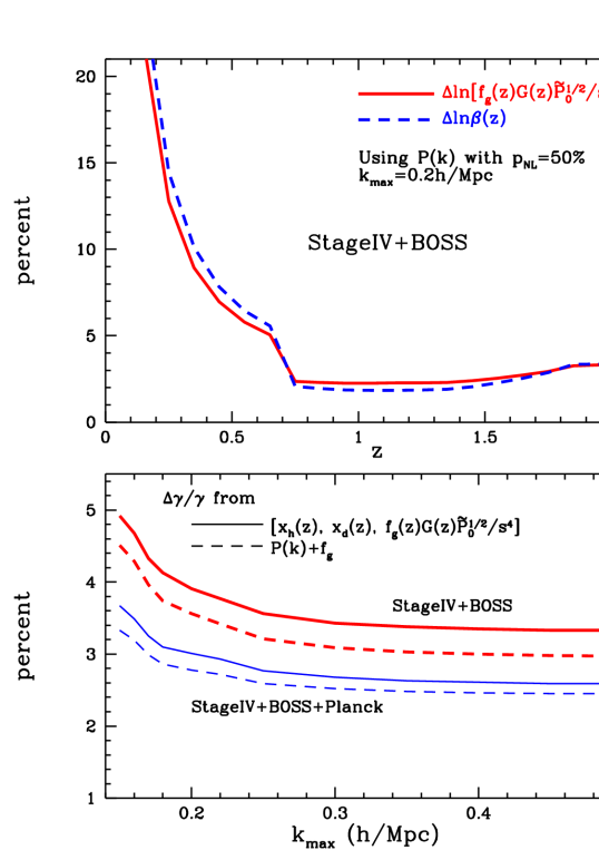
Figure 2: Top: uncertainties on $f_{g}(z)G(z)\tilde{P}_{0}^{1/2}/s^{4}$ and $\beta(z)$ for StageIV+BOSS per $\Delta z=0.1$ redshift bin. Bottom: uncertainties on the growth rate powerlaw index $\gamma$ for StageIV+BOSS, with and without Planck priors.

The bottom panel of Fig.2 shows the uncertainties on the growth rate powerlaw index $\gamma$ for StageIV+BOSS, with and without Planck priors. Note that $\gamma$ is defined by parametrizing the growth rate as a powerlaw (Wang & Steinhardt, 1998; Lue, Scoccimarro, & Starkman, 2004),

$$f_{g}(z)=\left[\Omega_{m}(a)\right]^{\gamma},$$ (37)

where $\Omega_{m}(a)=8\pi G\rho_{m}(a)/(3H^{2})$. The solid lines in the bottom panel of Fig.2 show the precision on $\gamma$ using only the $\{x_{h}(z),x_{d}(z),f_{g}(z)\sigma_{m}(z)/s^{4}\}$ measured from $P(k)$ and marginalized over all other parameters. The dashed lines show the precision on $\gamma$ when the full $P(k)$ is used, including the growth information (i.e., the ”$P(k)+f_{g}$” method).

3.3 Dark Energy Figure of Merit

To calculate the DETF dark energy FoM (Albrecht et al., 2006), FoM$=1/\sqrt{\mbox{det}[{\rm Cov}(w_{0},w_{a})]}$ (Wang, 2008b), we need to project our large set of measured parameters into the standard set of $\{w_{0},w_{a},\Omega_{X},\Omega_{k},\omega_{m},\omega_{b},n_{s},\ln A_{s}\}$.

The BAO only method gives measurement of $\{x_{h}(z_{i}),x_{d}(z_{i})\}$ from each redshift slice. The Fisher matrix for these measurements are then projected into the Fisher matrix for $\{w_{0},w_{a},\Omega_{X},\Omega_{k},\omega_{m},\omega_{b}\}$. Because the dependence on $\{\omega_{m},\omega_{b}\}$ only comes through $s$, $\omega_{m}$ and $\omega_{b}$ are perfectly degenerate if no priors are added. This can be shown explicitly by computing the submatrix for $\{\omega_{m},\omega_{b}\}$ in the Fisher matrix, which is proportional to

$$\left(\begin{array}[]{cc}\left(\frac{\partial\ln x_{h}}{\partial\omega_{m}}\right)^{2}&\left(\frac{\partial\ln x_{h}}{\partial\omega_{m}}\right)\left(\frac{\partial\ln x_{h}}{\partial\omega_{b}}\right)\\ \left(\frac{\partial\ln x_{h}}{\partial\omega_{m}}\right)\left(\frac{\partial\ln x_{h}}{\partial\omega_{b}}\right)&\left(\frac{\partial\ln x_{h}}{\partial\omega_{b}}\right)^{2}\end{array}\right)$$ (40)

the determinant of this submatrix is zero, thus the determinant of the entire Fisher matrix for $\{w_{0},w_{a},\Omega_{X},\Omega_{k},\omega_{m},\omega_{b}\}$ is zero. It can be shown that the combination determined by the BAO only method is

$$\tilde{\omega}_{m} \equiv \omega_{m}+\omega_{b}\,\left(\frac{\partial\ln x_{h}}{\partial\omega_{b}}\right)\left(\frac{\partial\ln x_{h}}{\partial\omega_{m}}\right)^{-1}$$ (41)

$$= \omega_{m}+\omega_{b}\,\left(\frac{\partial\ln s}{\partial\omega_{b}}\right)\left(\frac{1}{2\omega_{m}}+\frac{\partial\ln s}{\partial\omega_{m}}\right)^{-1}$$

It can be shown explicitly that the Fisher matrix for $\{w_{0},w_{a},\Omega_{X},\Omega_{k},\tilde{\omega}_{m}\}$ is exactly the same as the $\{w_{0},w_{a},\Omega_{X},\Omega_{k},\omega_{m}\}$ submatrix of the original Fisher matrix for $\{w_{0},w_{a},\Omega_{X},\Omega_{k},\omega_{m},\omega_{b}\}$. Thus to compute the FoM for BAO only, one only needs to drop the Fisher matrix elements for $\omega_{b}$, then invert the resultant Fisher matrix to obtain the covariance matrix. Note that the Fisher matrix for $\{w_{0},w_{a},\Omega_{X},\Omega_{k},\omega_{m},\omega_{b}\}$ should be used when combining with Planck priors.

There are four different ways that we can extract dark energy information from the $P(k)$ method (in the order of increasing information content):
(1) $\{x_{h}(z),x_{d}(z)\}$ from $P(k)$: Project the Fisher matrix for $\{\ln H(z_{i})$, $\ln D_{A}(z_{i})$, $\ln[f_{g}(z_{i})\sigma_{m}(z_{i})]$; $\omega_{m}$, $\omega_{b}$, $n_{s}\}$ into that of $\{\ln x_{h}(z_{i})$, $\ln x_{d}(z_{i})$, $\ln[f_{g}(z_{i})\sigma_{m}(z_{i})/s^{4}]$; $\omega_{m}$, $\omega_{b}$, $n_{s}\}$ (see Sec.3.2), then marginalize over $\{\ln[f_{g}(z_{i})\sigma_{m}(z_{i})/s^{4}];\omega_{m},\omega_{b},n_{s}\}$, and project the Fisher matrix for $\{\ln x_{h}(z_{i}),\ln x_{d}(z_{i})\}$ into the standard set of cosmological parameters.
(2) $\{x_{h}(z),x_{d}(z),f_{g}(z)\sigma_{m}(z)/s^{4}\}$ from ${\boldmath P(k)}$: Project the Fisher matrix for $\{\ln H(z_{i})$, $\ln D_{A}(z_{i})$, $\ln[f_{g}(z_{i})\sigma_{m}(z_{i})]$; $\omega_{m}$, $\omega_{b}$, $n_{s}\}$ into that of $\{\ln x_{h}(z_{i})$, $\ln x_{d}(z_{i})$, $\ln[f_{g}(z_{i})\sigma_{m}(z_{i})/s^{4}]$; $\omega_{m}$, $\omega_{b}$, $n_{s}\}$ (see Sec.3.2), then marginalize over $\{\omega_{m},\omega_{b},n_{s}\}$, and project the Fisher matrix for $\{\ln x_{h}(z_{i}),\ln x_{d}(z_{i}),\ln[f_{g}(z_{i})\sigma_{m}(z_{i})/s^{4}]\}$ into the standard set of cosmological parameters.
(3) ${\boldmath P(k)}$ marginalized over ${\boldmath f_{g}}$: Marginalize over $\ln[f_{g}(z_{i})\sigma_{m}(z_{i})]$ to obtain the Fisher matrix for $\{\ln H(z_{i}),\ln D_{A}(z_{i});\omega_{m},\omega_{b},n_{s}\}$, and project it into the standard set of cosmological parameters.
(4) ${\boldmath P(k)+f_{g}}$: Project the Fisher matrix for $\{\ln H(z_{i})$, $\ln D_{A}(z_{i})$, $\ln[f_{g}(z_{i})\sigma_{m}(z_{i})]$; $\omega_{m}$, $\omega_{b}$, $n_{s}\}$ into the standard set of cosmological parameters.

Fig.3 shows the DETF dark energy FoM for StageIV+BOSS, without (top panel) and with (bottom panel) Planck priors, as a function of the nonlinear cutoff $k_{max}$. The four methods of using $P(k)$ described above, as well as the BAO only method, are shown. Note that the FoMs from the three most conservative methods, BAO only, $\{x_{h}(z),x_{d}(z)\}$ from $P(k)$, and $\{x_{h}(z),x_{d}(z),f_{g}(z)\sigma_{m}(z)/s^{4}\}$ from $P(k)$, are insensitive to the increase of $k_{max}$ for $k_{max}\mathrel{\mathchoice{\lower 3.6pt\vbox{\halign{$\mathsurround=0pt\displaystyle\hfill#\hfil$\cr>\crcr\sim\crcr}}}{\lower 3.6pt\vbox{\halign{$\mathsurround=0pt\textstyle\hfill#\hfil$\cr>\crcr\sim\crcr}}}{\lower 3.6pt\vbox{\halign{$\mathsurround=0pt\scriptstyle\hfill#\hfil$\cr>\crcr\sim\crcr}}}{\lower 3.6pt\vbox{\halign{$\mathsurround=0pt\scriptscriptstyle\hfill#\hfil$\cr>\crcr\sim\crcr}}}}0.3h/$Mpc. We have not included the nonlinearity in the RSD due to peculiar velocities here for simplicity. Adding a peculiar velocity of 300 km/s is equivalent to adding $0.001$ in quadrature to the redshift dispersion $\sigma_{z}=0.001(1+z)$; this has a negligible effect on the FoM for StageIV+BOSS, since the FoM is most sensitive to assumptions about the Stage IV survey, which is at $z\geq 0.7$.

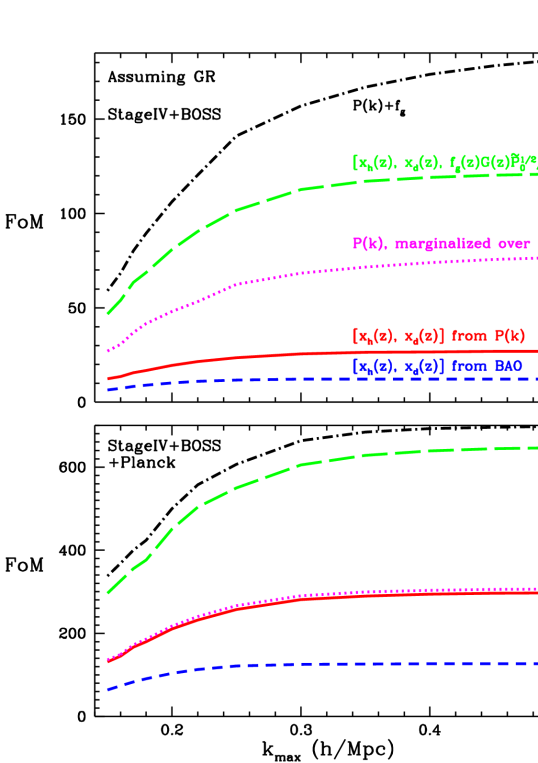
Figure 3: Dark energy FoM for StageIV+BOSS, without (top panel) and with (bottom panel) Planck priors, as a function of the nonlinear cutoff $k_{max}$.

The most conservative of the $P(k)$ approaches, using $\{x_{h}(z),x_{d}(z)\}$ measured from $P(k)$ and marginalized over all other parameters, gives a dark energy FoM about a factor of two larger than that of the BAO only method, with or without Planck priors. This provides a robust conservative method to go beyond BAO only in extracting dark energy information from galaxy clustering data.

It is interesting to note that $\{x_{h}(z),x_{d}(z)\}$ from $P(k)$ (solid line) gives similar dark energy FoM to that of the full $P(k)$ marginalized over growth information (dotted line), when Planck priors are included. Similarly, $\{x_{h}(z),x_{d}(z),f_{g}(z)\sigma_{m}(z)/s^{4}\}$ gives dark energy FoM close to that of the full $P(k)$ with growth information included, when Planck priors are added.

3.4 Comparison With Previous Work

This work has the most overlap with Wang et al. (2010), which explored the optimization of a space-based galaxy redshift survey. The differences of this work from Wang et al. (2010) are:
(1) This work presents a new conservative approach to extract dark energy constraints from galaxy clustering data: the use of only the $H(z)s$ and $D_{A}(z)/s$ measurements from the observed galaxy power spectrum, $P_{g}^{obs}(k)$, to probe dark energy. This bridges the methods using $P_{g}^{obs}(k)$ and the BAO method (which uses $H(z)s$ and $D_{A}(z)/s$ measurements from fitting the BAO peaks).
(2) This work presents a new combination of growth information, $f_{g}(z)G(z)/s^{4}$, that can be measured nearly as precisely as the linear redshift-space distortion parameter $\beta$ (see Fig.2), but can be used to probe the growth history of cosmic large scale structure without assuming a bias model. Wang et al. (2010) did not study growth constraints explicitly; they either marginalized over the growth rate information, or assumed that gravity is described by general relativity.
(3) This work focuses on model-independent constraints of dark energy and gravity in terms of $H(z)s$, $D_{A}(z)/s$, and $f_{g}(z)G(z)/s^{4}$ measured in $\Delta z=0.1$ redshift bins. Wang et al. (2010) focuses on the conventional dark energy model with dark energy equation of state given by $w_{X}(z)=w_{0}+w_{a}(1-a)$ (Chevallier & Polarski, 2001), and dark energy density function $X(z)=\rho_{X}(z)/\rho_{X}(0)$ parametrized by its value at $z=2/3$, 4/3, and 2.

The methodology developed in this work differs from what is currently used in analyzing galaxy clustering data. This work proposes the simultaneous measurement of $H(z)s$, $D_{A}(z)/s$, and $f_{g}(z)G(z)/s^{4}$ from galaxy clustering data without imposing any priors. Because of the limited volume probed by current data, no simultaneous measurements of $H(z)$, $D_{A}(z)$, and $f_{g}(z)$ have been made without imposing strong priors on cosmological parameters. The first simultaneous measurements of $H(z)s$ and $D_{A}(z)/s$ were made by Chuang & Wang (2011) at $z_{eff}=0.35$ using SDSS DR7 LRG data; they marginalized over growth information. Blake et al. (2011) measured $f_{g}(z)\sigma_{8}(z)$ at several redshifts while fixing the background cosmology. Most recently, Reid et al. (2012) published the first simultaneous measurement of $D_{A}(z)H(z)$, $D_{A}(z)^{2}/H(z)$, and $f_{g}(z)\sigma_{8}(z)$ at $z_{eff}=0.57$ using BOSS data, assuming WMAP7 priors.

This work presents forecasts of the precision of the most general measurements of cosmic expansion history (via $H(z)$ and $D_{A}(z)$) and gravity (via $f_{g}(z)G(z)$) that can be made from a Stage IV galaxy redshift survey. These will be the most model-independent results on probing dark energy and probing gravity from such a survey.

4 Summary and Discussion

We have examined how the constraints on the scaled expansion history of the universe, $x_{h}(z)=H(z)s$, and the scaled angular diameter distance, $x_{d}(z)=D_{A}(z)/s$, depend on the methods used to analyze the galaxy clustering data. We find that using the observed galaxy power spectrum, $P_{g}^{obs}(k)$, $x_{h}(z)$ and $x_{d}(z)$ are measured more accurately and are significantly less correlated with each other, compared to using only the information from the baryon acoustic oscillations (BAO) in $P_{g}^{obs}(k)$ (see Fig.1). Using the $\{x_{h}(z),x_{d}(z)\}$ from $P_{g}^{obs}(k)$ gives a DETF dark energy FoM approximately a factor of two larger than using the $\{x_{h}(z),x_{d}(z)\}$ from BAO only (see Fig.3); this provides a robust conservative method to go beyond BAO only in extracting dark energy information from galaxy clustering data. This is encouraging since Chuang & Wang (2011) found that $\{x_{h}(z),x_{d}(z)\}$ from SDSS galaxy clustering data are not sensitive to systematic uncertainties.

Furthermore, we find that if the redshift-space distortion information contained in $P_{g}^{obs}(k)$ is used, we can measure $\{x_{h}(z),x_{d}(z),f_{g}(z)G(z)\tilde{P}_{0}^{1/2}/s^{4}\}$ with high precision from a Stage IV galaxy redshift survey with $0.7<z<2$ over 15,000 (deg)² (see Figs.1 and 2), where $f_{g}(z)$ and $G(z)$ are linear growth rate and growth factor of large scale structure respectively, and $\tilde{P}_{0}$ denotes the dimensionless normalization of $P_{m}^{lin}(k|z=0)$ . Adding $f_{g}(z)G(z)\tilde{P}_{0}^{1/2}/s^{4}$ to $\{x_{h}(z),x_{d}(z)\}$ significantly boosts the dark energy FoM, compared to using $\{x_{h}(z),x_{d}(z)\}$ only, or using $P_{g}^{obs}(k)$ marginalized over the growth information, assuming that gravity is not modified (see Fig.3). Alternatively, $f_{g}(z)G(z)\tilde{P}_{0}^{1/2}/s^{4}$ provides a powerful test of gravity, as dark energy and modified gravity models that give identical $H(z)$ likely give different $f_{g}(z)$ (Wang, 2008a). Measuring $\{x_{h}(z),x_{d}(z),f_{g}(z)G(z)\tilde{P}_{0}^{1/2}/s^{4}\}$ simultaneously allows us to probe gravity without fixing the background cosmological model. We will be adopting this approach to analyze simulated and real galaxy redshift catalogs in future work.

We have developed a conservative approach to analyzing galaxy clustering data that should be insensitive to systematic uncertainties, if only data on quasi-linear scales are used ($k_{max}\mathrel{\mathchoice{\lower 3.6pt\vbox{\halign{$\mathsurround=0pt\displaystyle\hfill#\hfil$\cr<\crcr\sim\crcr}}}{\lower 3.6pt\vbox{\halign{$\mathsurround=0pt\textstyle\hfill#\hfil$\cr<\crcr\sim\crcr}}}{\lower 3.6pt\vbox{\halign{$\mathsurround=0pt\scriptstyle\hfill#\hfil$\cr<\crcr\sim\crcr}}}{\lower 3.6pt\vbox{\halign{$\mathsurround=0pt\scriptscriptstyle\hfill#\hfil$\cr<\crcr\sim\crcr}}}}0.2h/$Mpc). Since the dark energy FoM (see Fig.3) and the gravity constraints (see lower panel of Fig.2) are insensitive to the inclusion of smaller scale information at $k_{max}\mathrel{\mathchoice{\lower 3.6pt\vbox{\halign{$\mathsurround=0pt\displaystyle\hfill#\hfil$\cr>\crcr\sim\crcr}}}{\lower 3.6pt\vbox{\halign{$\mathsurround=0pt\textstyle\hfill#\hfil$\cr>\crcr\sim\crcr}}}{\lower 3.6pt\vbox{\halign{$\mathsurround=0pt\scriptstyle\hfill#\hfil$\cr>\crcr\sim\crcr}}}{\lower 3.6pt\vbox{\halign{$\mathsurround=0pt\scriptscriptstyle\hfill#\hfil$\cr>\crcr\sim\crcr}}}}0.3h/$Mpc, our results are likely robust indicators of how well a Stage IV galaxy redshift survey can probe dark energy and constrain gravity.

In analyzing real data, the systematic effects (bias between luminous matter and matter distributions, nonlinear effects, and redshift-space distortions) will ultimately need to be modeled in detail and reduced where possible (see, e.g., Percival et al. (2010); Blake et al. (2011); Padmanabhan et al. (2012)). This will require cosmological N-body simulations that include galaxies, either by incorporating physical models of galaxy formation (see, e.g., Baugh (2006); Angulo et al. (2008)), or using halo occupation distributions (HOD) measured from the largest available data sets (see, e.g., Zheng et al. (2009), and http://lss.phy.vanderbilt.edu/lasdamas/overview.html). We can expect a Stage IV galaxy redshift survey to play a critical role in advancing our understanding of cosmic acceleration within the next decade.

References

- (1)
- Albrecht et al. (2006) Albrecht, A.; et al., Report of the Dark Energy Task Force, astro-ph/0609591
- Albrecht et al. (2009) Albrecht, A.; et al., Findings of the Joint Dark Energy Mission Figure of Merit Science Working Group, arXiv:0901.0721
- Anderson et al. (2012) Anderson, L., et al., 2012, arXiv:1203.6594
- Angulo et al. (2008) Angulo, R., Baugh, C. M., Frenk, C. S., Lacey, C. G. 2008, MNRAS, 383, 755
- Baugh (2006) Baugh, C. M. 2006, Reports on Progress in Physics, 69, 3101.
- Blake & Glazebrook (2003) Blake, C.; Glazebrook, G., 2003, ApJ, 594, 665
- Blake et al. (2011) Blake, C., et al., 2011, MNRAS, 415.2876
- Chevallier & Polarski (2001) Chevallier, M., & Polarski, D. 2001, Int. J. Mod. Phys. D10, 213
- Chuang & Wang (2011) Chuang, C.-H.; & Wang, Y., arXiv:1102.2251
- Eisenstein & Hu (1998) Eisenstein D, Hu W;1998;ApJ;496;605
- Feldman, Kaiser, & Peacock (1994) Feldman, H.A., Kaiser, N., Peacock, J.A., 1994, ApJ, 426, 23
- Geach et al. (2010) Geach, J. E.; et al., 2010, MNRAS, 402, 1330
- Guzzo et al. (2008) Guzzo L et al., Nature 451, 541 (2008)
- Hamilton (1998) Hamilton, A. J. S., in ”The Evolving Universe” ed. D. Hamilton, Kluwer Academic, p. 185-275 (1998)
- Heavens (2009) Heavens, A, 2009, NuPhS, 194, 76
- Hu & Sugiyama (1996) Hu, W., & Sugiyama, N. 1996, ApJ, 471, 542
- Kaiser (1987) Kaiser N;1987;MNRAS;227;1
- Knox, Song, & Tyson (2006) Knox, L., Song, Y.-S., & Tyson, J.A., Phys.Rev.D74:023512,2006
- Laureijs et al. (2011) Laureijs, R., et al., “Euclid Definition Study Report”, arXiv:1110.3193
- Lue, Scoccimarro, & Starkman (2004) Lue A, Scoccimarro R, Starkman G D;2004;PRD;69;124015
- Majumdar & Mohr (2004) Majumdar, S.; Mohr, J.J., Astrophys.J.613:41-50,2004
- Manera & Mota (2006) Manera, M.; Mota, D.F., Mon.Not.Roy.Astron.Soc.371:1373,2006
- Matarrese, Verde, & Heavens (1997) Matarrese, S., Verde, L., Heavens, A. F., 1997, MNRAS, 290, 651
- Mota (2008) Mota, D.F., JCAP 09 : 006 (2008)
- Mukherjee et al. (2008) Mukherjee, P.; Kunz, M.; Parkinson, D.; Wang, Y., PRD, 78, 083529 (2008)
- Orsi et al. (2010) Orsi, A.; et al., 2010, MNRAS, 405, 1006
- Padmanabhan et al. (2012) Padmanabhan, N.; et al., arXiv:1202.0090
- Percival et al. (2010) Percival, W. J., et al., 2010, MNRAS, 401, 2148
- Perlmutter et al. (1999) Perlmutter, S. et al., 1999, ApJ, 517, 565
- Reid et al. (2012) Reid, B.A., et al., 2012, arXiv:1203.6641
- Riess et al. (1998) Riess, A. G, et al., 1998, Astron. J., 116, 1009
- Sartoris et al. (2011) Sartoris, B.; Borgani, S.; Rosati, P.; Weller, J., arXiv:1112.0327
- Seo & Eisenstein (2003) Seo H, Eisenstein D J;2003;ApJ;598;720
- Seo & Eisenstein (2007) Seo, H., & Eisenstein, D. J. 2007, ApJ, 665, 14 [SE07].
- Song & Percival (2009) Song, Y.-S., & Percival, W. J., JCAP 0910:004,2009
- Spergel et al. (2007) Spergel, D. N., et al., ApJS, 170 (2007), p. 377
- Tegmark (1997) Tegmark M;1997;PRL;79;3806
- Verde et al. (2002) Verde, L. et al.;2002;MNRAS;335;432
- Wang & Steinhardt (1998) Wang, L.; Steinhardt, P.J.;1998;ApJ;508;483
- Wang (2006) Wang, Y., 2006, ApJ, 647, 1
- Wang (2008a) Wang, Y., 2008a, JCAP, 0805, 021
- Wang (2008b) Wang, Y., 2008b, Phys. Rev. D 77, 123525
- Wang (2010a) Wang, Y., MPLA, 25, 3093 (2010a)
- Wang (2010b) Wang, Y., Dark Energy, Wiley-VCH (2010b)
- Wang et al. (2010) Wang, Y.; et al., MNRAS, 409, 737 (2010)
- Weinberg et al. (2012) Weinberg, D.H.; et al., arXiv:1201.2434
- Zhang et al. (2007) Zhang, P.; Liguori, M.; Bean, R.; & Dodelson. S. 2007, Phys.Rev.Lett. 99, 141302
- Zheng et al. (2009) Zheng, Z.; et al., 2009, ApJ, 707, 554Z