Post-Double Hopf Bifurcation Dynamics and Adaptive Synchronization of a Hyperchaotic System

Abstract

In this paper a four-dimensional hyperchaotic system with only one equilibrium is considered and its double Hopf bifurcations are investigated. The general post-bifurcation and stability analysis are carried out using the normal form of the system obtained via the method of multiple scales. The dynamics of the orbits predicted through the normal form comprises possible regimes of periodic solutions, two-period tori, and three-period tori in parameter space.

Moreover, we show how the hyperchaotic synchronization of this system can be realized via an adaptive control scheme. Numerical simulations are included to show the effectiveness of the designed control.

1 Introduction

In the last decades study of hyperchaos has received great attention due to its important role in nonlinear science [19, 13, 22]. Several hyperchaotic systems with more than one positive Lyapunov exponent have been constructed via control techniques.

In this paper we consider a four dimensional dynamical system firstly introduced in [9]. This system was constructed by adding a linear feedback controller to the second equation of the chaotic Chen system [5] and an additional new state equation. The rich dynamics of this modified driven Chen system has been observed in [10] via computer simulations showing both chaotic and hyperchaotic attractors and period-doubling bifurcations.

The aim of this paper is, from one hand, to understand better the onset of the hyperchaos by the investigation of double Hopf bifurcation of the system and the analysis of the post-bifurcation dynamics via the normal form theory [14], [15]. From the other hand we want to realize both the chaotic and the hyperchaotic synchronization of the system designing a global adaptive controller.

We will use in Section 3 a perturbation technique, essentially based on multiple scales method, to compute the post-double Hopf normal form [23, 24, 25]. This method does not need the application of the Center Manifold Theory and can be employed with the aid of symbolic computation [26, 27].

Numerical simulations are performed to corroborate the predictions from the normal form, revealing the existence of stable periodic and toroidal attractors in the post-supercritical-Hopf cases.

Moreover, since the interest into synchronization of hyperchaotic systems has been always increasing, in particular due to its applications in secure communications (in fact the presence of more than one Lyapunov exponent generates more complex dynamics and improves the security), we propose a scheme to synchronize the modified hyperchaotic Chen system via adaptive control. Recently, many methods and techniques have been developed to realize synchronization and control of chaotic systems, see references [17, 11, 12, 7, 18, 29] and [3] for a review. In the same spirit of [16], in Section 4 we design an adaptive control law and an update rule for uncertain parameters based on Lyapunov stability theory.

Numerical simulations are presented to verify the effectiveness of the proposed synchronization method both in chaotic and hyperchaotic regime.

2 Linear analysis and double Hopf bifurcations

Let us consider the following modified Chen system, firstly obtained in [9]:

$$\left\{\begin{array}[]{l}\dot{x_{1}}=a(x_{2}-x_{1})\\ \dot{x_{2}}=-dx_{1}-x_{1}x_{3}+cx_{2}-x_{4}\\ \dot{x_{3}}=x_{1}x_{2}-bx_{3}\\ \dot{x_{4}}=x_{1}+k\end{array}\right.$$ (2.1)

where $a,b,c,d$ and $k$ are real constants.

Once introduced the following coordinates transformations:

$$x=x_{1}+k,\ \ y=y_{1}+k,\ \ z=x_{3}-\frac{k^{2}}{b},\ \ w=x=x_{4}-k\left(d-c+\frac{k^{2}}{b}\right),$$

which translate to the origin the only equilibrium $E$:

$$E\equiv\left(-k,-k,\frac{k^{2}}{b},k\left(d-c+\frac{k^{2}}{b}\right)\right),$$ (2.2)

the system (2.1) becomes:

$$\left\{\begin{array}[]{l}\dot{x}=a(y-x)\\ \dot{y}=-dx-xz+cy-w-\displaystyle\frac{k^{2}}{b}x+kz\\ \dot{z}=xy-bz-k(x+y)\\ \dot{w}=x\end{array}\right.$$ (2.3)

By choosing the values of parameters $a=36,\,b=3,\,c=28$ and $d=-16$ the origin is unstable and $\nabla V=-a-b+c<0$. Therefore the system is dissipative and the trajectories converge to an attractor which is hyperchaotic, as shown in Fig. 1.

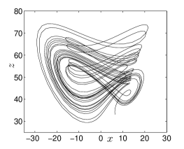
Figure 1: The parameters are chosen as $a=36,\,b=3,\,c=28,d=-16$ and $k=1$. (a) The hyperchaotic attractor. (b) The dynamics of the Lyapunov exponents: the system admits two positive Lyapunov exponents.

Several bifurcation routes to hyperchaos from periodic, quasi-periodic and chaotic orbits are observed in [10] via computer simulations. Since there exists only one equilibrium point, the possibility of the fixed point undergoing transcritical, pitchfork or saddle-node bifurcations (all of which involve creation, annihilation or exchange of stability of a pair of equilibria) is precluded. Thus the origin can be only destabilized via a Hopf or double Hopf bifurcation.

Applying the Routh-Hurwitz criterion one gets the following conditions for the origin being a stable equilibrium:

$$a_{3}>0,\ \ a_{0}>0,\ \ a_{3}a_{2}-a_{1}>0,\ \ a_{3}(a_{2}a_{1}-a_{3}a_{0})-a_{1}^{2}>0,$$ (2.4)

where:

$$a_{3} = a+b-c$$

$$a_{2} = ab+\frac{ak^{2}}{b}-ac+ad-bc+k^{2}$$

$$a_{1} = a(-bc+bd+3k^{2}+1)$$

$$a_{0} = ab$$

are the coefficients of the characteristic polynomial $p(\lambda)=\lambda^{4}+a_{3}\lambda^{3}+a_{2}\lambda^{2}+a_{1}\lambda+a_{0}$.

Since the post-bifurcation dynamics following regular Hopf bifurcation in this modified Chen system has been recently studied in [4], we are interested into double Hopf bifurcations. At the double Hopf bifurcation the four eigenvalues of the linearized system must be two pairs of purely imaginary complex conjugates $\lambda_{1,2}=\pm i\sigma_{1},\lambda_{3,4}=\pm i\sigma_{2}$ and the characteristic equation must have the form $(\lambda^{2}+\sigma_{1}^{2})(\lambda^{2}+\sigma_{2}^{2})=0$, which leads to the following conditions for a double Hopf bifurcation to occur:

$$\begin{array}[]{lllll}a_{3}=0,\\ a_{2}=\sigma_{1}^{2}+\sigma_{2}^{2}>0,\\ a_{1}=0,\\ a_{0}=\sigma_{1}^{2}\sigma_{2}^{2}>0,\\ a_{2}^{2}-4a_{0}>0.\end{array}\qquad\Rightarrow\qquad\begin{array}[]{llll}c=c^{*}=a+b,\\ d=d^{*}=a+b-\displaystyle\frac{1}{b}(3k^{2}+1),\\ k^{2}>\displaystyle\frac{a+b^{3}+2b\sqrt{ab}}{b-2a},\\ \sigma_{1},\sigma_{2}\in\mathbb{R},\end{array}$$ (2.5)

both for $a,b>0$ and $b>2a$ or $a,b<0$ and $b<2a$.

3 Normal form and general post-bifurcation dynamics

To compute the normal form of the modified Chen system (2.3) we will use a perturbation technique based on the multiple scales method [15, 23, 27].

Near the double Hopf bifurcation different time scales $T_{j}=\varepsilon^{j}t,\,j=0,1,2,\dots$ can be distinguished and therefore the time derivative decouples as follows:

$$\frac{d}{dt}=\frac{\partial}{\partial T_{0}}+\varepsilon\frac{\partial}{\partial T_{1}}+\varepsilon^{2}\frac{\partial}{\partial T_{2}}+\varepsilon^{3}\frac{\partial}{\partial T_{3}}\dots$$ (3.1)

Let us write the solutions of the original system (2.3) and the bifurcation parameters as nonlinear expansions in $\varepsilon$:

$$x=\varepsilon x_{1}+\varepsilon^{2}x_{2}+\varepsilon^{3}x_{3}+O(\varepsilon^{4}), y=\varepsilon y_{1}+\varepsilon^{2}y_{2}+\varepsilon^{3}y_{3}+O(\varepsilon^{4}),$$

$$z=\varepsilon z_{1}+\varepsilon^{2}z_{2}+\varepsilon^{3}z_{3}+O(\varepsilon^{4}), w=\varepsilon w_{1}+\varepsilon^{2}w_{2}+\varepsilon^{3}w_{3}+O(\varepsilon^{4}),$$ (3.2)

$$c=c^{*}+\varepsilon c_{1}+\varepsilon^{2}c_{2}+\varepsilon^{3}c_{3}+O(\varepsilon^{4}), d=d^{*}+\varepsilon d_{1}+\varepsilon^{2}d_{2}+\varepsilon^{3}d_{3}+O(\varepsilon^{4}),$$

where $c^{*},d^{*}$ are the bifurcation values at the double Hopf singularity as calculated in (2.5). All the expansion coefficients $x_{i},y_{i},z_{i}$ and $w_{i},\,i=1,2,3,\dots$ depend on the time scales $T_{j},\,j=0,1,2,\dots$.

Substituting all the above expansions (3.1)-(3.2) into the system (2.3) and collecting the terms at each order in $\varepsilon$, one gets a sequence of differential systems for the $x_{i},y_{i},z_{i}$ and $w_{i},\,i=1,2,3,\dots$:

$$O(\varepsilon) : \hskip 65.44142pt\mathcal{L}w_{1}=0,$$ (3.3)

$$O(\varepsilon^{2}) : \hskip 65.44142pt\mathcal{L}w_{2}=\Gamma_{2},$$ (3.4)

$$O(\varepsilon^{3}) : \hskip 65.44142pt\mathcal{L}w_{3}=\Gamma_{3},$$ (3.5)

where $\mathcal{L}$ is the following linear operator:

$$\mathcal{L} = \frac{1}{k}\left(\frac{1}{a}\frac{\partial^{4}}{\partial T_{0}^{4}}+\left(1+\frac{b-c^{*}}{a}\right)\frac{\partial^{3}}{\partial T_{0}^{3}}+\left(\frac{k^{2}-bc^{*}}{a}+\frac{k^{2}}{b}+b-c^{*}+d^{*}\right)\frac{\partial^{2}}{\partial T_{0}^{2}}\right.$$ (3.6)

$$+\left.(1-bc^{*}+bd^{*}+3k^{2})\frac{\partial}{\partial T_{0}}+b\right)$$

and the source terms $\Gamma_{2}$ and $\Gamma_{3}$ contains the nonlinear terms. The equations for $x_{i},y_{i}$ and $z_{i}$ can be easily obtained only in terms of $w_{i}$, but here we skip all the calculation details.

The solution of the linear homogeneous problem (3.3) is given by:

$$w_{1}=\sum_{j=1}^{2}\left(\alpha_{j}(T_{k})e^{i\sigma_{j}T_{0}}+\bar{\alpha}_{j}(T_{k})e^{-i\sigma_{j}T_{0}}\right),$$ (3.7)

where the fields $\alpha_{j}$, depending on the time scales $T_{k},\,k=1,2,\dots$, lie on the center manifolds and $\bar{\alpha}_{j}$ represent their complex conjugate fields. The real numbers $\sigma_{j}$ are the imaginary parts of the pairs of purely imaginary complex eigenvalues calculated at the double Hopf singularity. Suppressing the secular terms appearing in $\Gamma_{2}$ only by imposing $T_{1}=0$ and $c_{1},d_{1}=0$ one gets the solutions $w_{2}$.

The solvability condition at $O(\varepsilon^{3})$ leads to the following two coupled equations for the fields $\alpha_{1}$ and $\alpha_{2}$:

$$\frac{\partial\alpha_{j}}{\partial T_{2}}=L^{(j)}\alpha_{j}+M^{(j)}\alpha_{j}^{2}\bar{\alpha}_{j}+N^{(j)}\alpha_{1}\alpha_{2}\bar{\alpha}_{j},$$ (3.8)

where the coefficients $L^{(j)}$ are linearly dependent on the second order deviation $c_{2}$ and $d_{2}$ from the bifurcation values.

Using the polar coordinates $\alpha_{j}=\rho_{j}e^{i\vartheta_{j}},\ \bar{\alpha}_{j}=\rho_{j}e^{-i\vartheta_{j}}$, with $\rho_{j}$ and $\vartheta_{j}$ depending on $T_{2}$ and separating the real and the imaginary parts, one obtains the following normal form:

$$\frac{\partial\rho_{j}}{\partial T_{2}} = \rho_{j}\left(L_{11}^{(j)}c_{2}+L_{12}^{(j)}d_{2}+M_{1}^{(j)}\rho_{j}^{2}+N_{1}^{(j)}\rho_{(-j+3)}^{2}\right),$$ (3.9)

$$\frac{\partial\vartheta_{j}}{\partial T_{2}} = L_{21}^{(j)}c_{2}+L_{22}^{(j)}d_{2}+M_{2}^{(j)}\rho_{j}^{2}+N_{2}^{(j)}\rho_{(-j+3)}^{2}.$$ (3.10)

The explicit expression of the coefficients $L_{1l}^{(j)},L_{2l}^{(j)},M_{l}^{(j)}$ and $N_{l}^{(j)},\,l=1,2$ in terms of the parameters of the original system (2.3) can be found in [6].

The obtained normal form will be an analytical approximation of the periodic orbits at the double Hopf singularity.

The analysis of this normal form closely parallels earlier work by Yu and co-workers, in particular [25, 2].

The stationary solutions of the equations (3.9)-(3.10) are the following:

$$O : \rho_{1}=\rho_{2}=0,$$ (3.11)

$$H_{1} : \rho^{2}_{1}=-\displaystyle\frac{1}{M_{1}^{(1)}}\left(L_{11}^{(1)}c_{2}+L_{12}^{(1)}d_{2}\right),\ \rho_{2}=0,$$ (3.12)

$$\vartheta_{1}=L_{21}^{(1)}c_{2}+L_{22}^{(1)}d_{2}+M_{2}^{(1)}\rho_{1}^{2},$$

$$H_{2} : \rho_{1}=0,\ \rho_{2}^{2}=-\displaystyle\frac{1}{M_{1}^{(2)}}\left(L_{11}^{(2)}c_{2}+L_{12}^{(2)}d_{2}\right),$$ (3.13)

$$\vartheta_{2}=L_{21}^{(2)}c_{2}+L_{22}^{(2)}d_{2}+M_{2}^{(2)}\rho_{2}^{2},$$

$$T : \rho_{1}^{2}=\displaystyle\frac{-M_{1}^{(2)}\left(L_{11}^{(1)}c_{2}+L_{12}^{(1)}d_{2}\right)+N_{1}^{(1)}\left(L_{11}^{(2)}c_{2}+L_{12}^{(2)}d_{2}\right)}{M_{1}^{(1)}M_{1}^{(2)}-N_{1}^{(1)}N_{1}^{(2)}},$$ (3.14)

$$\rho_{2}^{2}=\displaystyle\frac{-M_{1}^{(1)}\left(L_{11}^{(2)}c_{2}+L_{12}^{(2)}d_{2}\right)+N_{1}^{(2)}\left(L_{11}^{(1)}c_{2}+L_{12}^{(1)}d_{2}\right)}{M_{1}^{(1)}M_{1}^{(2)}-N_{1}^{(1)}N_{1}^{(2)}},$$ (3.15)

$$\vartheta_{1}=L_{21}^{(1)}c_{2}+L_{22}^{(1)}d_{2}+M_{2}^{(1)}\rho_{1}^{2}+N_{2}^{(1)}\rho_{2}^{2},$$

$$\vartheta_{2}=L_{21}^{(2)}c_{2}+L_{22}^{(2)}d_{2}+M_{2}^{(2)}\rho_{2}^{2}+N_{2}^{(2)}\rho_{1}^{2}.$$

Performing a standard linear analysis of the system (3.9)-(3.10), it follows that the initial equilibrium state corresponding to $O$, is stable if:

$$L_{11}^{(j)}c_{2}+L_{12}^{(j)}d_{2}<0,\ {\rm for\ }j=1,2.$$ (3.16)

The conditions for the existence and stability of the stationary point $H_{1}$ (and consequently of a periodic solution for the system (2.3)) are:

$$M_{1}^{(1)}<0,$$ (3.17)

$$L_{11}^{(1)}c_{2}+L_{12}^{(1)}d_{2}>0,$$ (3.18)

$$L_{11}^{(2)}c_{2}+L_{12}^{(2)}d_{2}-\displaystyle\frac{N_{1}^{(2)}}{M_{1}^{(1)}}\left(L_{11}^{(1)}c_{2}+L_{12}^{(1)}d_{2}\right)<0.$$ (3.19)

Therefore along the critical line $l_{1}$:

$$l_{1}:\qquad L_{11}^{(1)}c_{2}+L_{12}^{(1)}d_{2}=0,\qquad L_{11}^{(2)}c_{2}+L_{12}^{(2)}d_{2}<0$$ (3.20)

the initial equilibrium bifurcates into a family of limit cycle (approximated by the periodic solution $H_{1}$) as follows from (3.16) and (3.18). Analogously, $H_{2}$ exists stable when:

$$M_{1}^{(2)}<0,$$ (3.21)

$$L_{11}^{(2)}c_{2}+L_{12}^{(2)}d_{2}>0,$$ (3.22)

$$L_{11}^{(1)}c_{2}+L_{12}^{(1)}d_{2}-\displaystyle\frac{N_{1}^{(1)}}{M_{1}^{(2)}}\left(L_{11}^{(2)}c_{2}+L_{12}^{(2)}d_{2}\right)<0,$$ (3.23)

and along the critical line $l_{2}$:

$$l_{2}:\qquad L_{11}^{(2)}c_{2}+L_{12}^{(2)}d_{2}=0,\qquad L_{11}^{(1)}c_{2}+L_{12}^{(1)}d_{2}<0$$ (3.24)

the initial equilibrium bifurcates into an other family of limit cycles given by the periodic solution $H_{2}$.

Finally, the conditions for the existence and stability of the point $T$ are the following:

$$N_{1}^{(1)}\left(L_{11}^{(2)}c_{2}+L_{12}^{(2)}d_{2}\right)-M_{1}^{(2)}\left(L_{11}^{(1)}c_{2}+L_{12}^{(1)}d_{2}\right)>0$$ (3.25)

$$N_{1}^{(2)}\left(L_{11}^{(1)}c_{2}+L_{12}^{(1)}d_{2}\right)-M_{1}^{(1)}\left(L_{11}^{(2)}c_{2}+L_{12}^{(2)}d_{2}\right)>0$$ (3.26)

$$M_{1}^{(1)}M_{1}^{(2)}-N_{1}^{(1)}N_{1}^{(2)}>0$$ (3.27)

$$M_{1}^{(2)}\left(L_{11}^{(1)}c_{2}+L_{12}^{(1)}d_{2}\right)\left(N_{1}^{(2)}-M_{1}^{(1)}\right)$$

$$\hskip 85.35826pt+M_{1}^{(1)}\left(L_{11}^{(2)}c_{2}+L_{12}^{(2)}d_{2}\right)\left(N_{1}^{(1)}-M_{1}^{(2)}\right)<0.$$ (3.28)

From the conditions (3.17)-(3.19) and (3.26) it follows that along the line $l_{3}$:

$$l_{3}:\left(L_{11}^{(2)}-\frac{N_{1}^{(2)}}{M_{1}^{(1)}}L_{11}^{(1)}\right)c_{2}+\left(L_{12}^{(2)}-\frac{N_{1}^{(2)}}{M_{1}^{(1)}}L_{12}^{(1)}\right)d_{2}=0,\quad{\rm and\ \eqref{H1stable1}-\eqref{H1stable2}\ hold}$$ (3.29)

the periodic solution $H_{1}$ bifurcates with frequency $\vartheta_{2}$ into a quasi-periodic solution (with a secondary Hopf bifurcation) and a 2-D torus arises. Analogously, taking into account (3.21)-(3.23) and (3.25), one individuates the line $l_{4}$:

$$l_{4}:\left(L_{11}^{(1)}-\frac{N_{1}^{(1)}}{M_{1}^{(2)}}L_{11}^{(2)}\right)c_{2}+\left(L_{12}^{(1)}-\frac{N_{1}^{(1)}}{M_{1}^{(2)}}L_{12}^{(2)}\right)d_{2}=0,\quad{\rm and\ \eqref{H2stable1}-\eqref{H2stable2}\ hold}$$ (3.30)

where the other periodic solution corresponding to $H_{2}$ bifurcates to the 2D motion with frequency $\vartheta_{1}$.

Finally, a 3D dynamical behavior can be even predicted when the following line $l_{5}$:

$$l_{5}: \left[L_{11}^{(1)}M_{1}^{(2)}\left(N_{1}^{(2)}-M_{1}^{(1)}\right)+L_{11}^{(2)}M_{1}^{(1)}\left(N_{1}^{(1)}-M_{1}^{(2)}\right)\right]c_{2}+$$

$$\left[L_{12}^{(1)}M_{1}^{(2)}\left(N_{1}^{(2)}-M_{1}^{(1)}\right)+L_{12}^{(2)}M_{1}^{(1)}\left(N_{1}^{(1)}-M_{1}^{(2)}\right)\right]d_{2}=0$$

is located between the lines $l_{3}$ and $l_{4}$ as follows from conditions (3.25)-(3.27).

In the post-double-Hopf bifurcation regime, the solutions exist on a torus in phase-space. The possible routes to chaos would most likely one of the quasiperiodic routes, i.e., either torus doubling via period doubling of the torus, or gradual torus breakdown, or the Ruelle-Takens route into chaos [15]. If the parameters are such that the system is locally very strongly dissipative or volume-contracting, intermittency is a possibility following bifurcations of the torus since the repulsion from the bifurcated (and now-unstable) torus may combine with volume contraction to set up a repulsion-reinjection intermittency scenario. However, this is less likely for most parameter sets than the previous three quasiperiodic routes. In exceptional cases, crises may also be possible, but again, this is much less likely for most system parameters than the quasiperiodic routes.

The modified Chen system (2.3) is next integrated for various parameters sets, showing the following three main behaviors:

1. the trajectories fly off to infinity;

2. the trajectories evolve towards a limit cycle;

3. the trajectories evolve to a strange attractor.

In all the numerical simulations the initial conditions are chosen to be close to the fixed point. The case 1., shown in Fig. 2, is realized at the parameter values $a=1,b=7$ and $k=9$ for which the double Hopf conditions are satisfied at $c^{*}=8$ and $d^{*}=-35$. Choosing $c_{2}=d_{2}=0.1$ the normal form (3.9)-(3.10) admits no stable fixed point (in particular the points $H_{2}$ and $T$ exist unstable, instead $H_{1}$ is complex) and it is not dissipative, therefore the trajectories fly off to infinity.

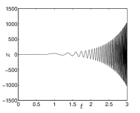
Figure 2: The time behavior of the state $x$ for the system (2.3).

The case 2. occurs for the parameter choice $a=1,b=3,k=-6.5$ (the critical parameter values are $c^{*}=4$ and $d^{*}=-38.5833$). Choosing the second order deviation $c_{2}=-19$ and $d_{2}=-20$ the system is strongly dissipative and the equilibrium point $H_{1}$ exists stable. The other two equilibria $H_{2}$ and $T$ are complex. Therefore our analysis predicts that the system states evolve towards a periodic orbit, in agreement with the simulation shown in Fig. 3.

Figure 3: The trajectories evolve towards a limit cycle.

Finally, for the choice $a=1,b=3,k=-7$ and the second order deviations $c_{2}=-3$ and $d_{2}=-3.6667$, no stable equilibria exist for the normal form (3.9)-(3.10) (in particular $H_{1}$ exists unstable and the equilibrium points $H_{2}$ and $T$ are complex). Due to the strong dissipativity, the numerical simulation in Fig. 4 shows that the trajectories evolve to a strange attractor.

Figure 4: The strange attractor in the $xyz$-space.

Note that other possible route to chaos can be investigated, e.g. in [6] the post-bifurcation dynamics in the context of two intermittent routes to chaos (routes following either subcritical or supercritical Hopf or double Hopf bifurcation) are observed.

4 Adaptive synchronization of the hyperchaotic system

The synchronization of two chaotic/hyperchaotic systems consists into designing a controller or forcing in such a way that the motion of each system can be adjusted to a common dynamics. The intrinsic nature of the chaotic systems does not obey to this idea of synchronization due to the sensitivity to initial conditions; in fact the trajectories of two identical chaotic systems evolve to completely different dynamical behavior when starting from different initial conditions (however they are close). Nevertheless, in the last decades, various synchronization methods have been proposed which show how it is possible to synchronize this kind of systems [1, 28, 8, 16, 3, 21].

In our case we want to realize a complete synchronization between two identical modified Chen system. The first one is the following master or driver system:

$$\left\{\begin{array}[]{l}\dot{x}_{m}=a(y_{m}-x_{m})\\ \dot{y}_{m}=-dx_{m}-xz_{m}+cy_{m}-w_{m}-\displaystyle\frac{k^{2}}{b}x_{m}+kz_{m}\\ \dot{z}_{m}=x_{m}y_{m}-bz_{m}-k(x_{m}+y_{m})\\ \dot{w}_{m}=x_{m}\end{array}\right.$$ (4.1)

and the second one is the slave or response system:

$$\left\{\begin{array}[]{l}\dot{x}_{s}=a_{1}(y_{s}-x_{s})+u_{1}\\ \dot{y}_{s}=-d_{1}x_{s}-xz_{s}+c_{1}y_{s}-w_{s}-\displaystyle\frac{k_{1}^{2}}{b_{1}}x_{s}+k_{1}z_{s}+u_{2}\\ \dot{z}_{s}=x_{s}y_{s}-b_{1}z_{s}-k_{1}(x_{s}+y_{s})+u_{3}\\ \dot{w}_{s}=x_{s}+u_{4}\end{array}\right.$$ (4.2)

whose evolution is guided by the controllers $u_{1},u_{2},u_{3}$ and $u_{4}$ and the parameters $a_{1},b_{1},c_{1},d_{1}$ and $k_{1}$ need to be estimated in such a way that the two systems (4.1) and (4.2) can be synchronized.

Our goal is to design suitable control functions $u_{i}$ and to find proper update rules for the parameters $a_{1},b_{1},c_{1},d_{1}$ and $k_{1}$ such that the response system globally synchronizes the driver system. This is equivalent to require that the error dynamical system, obtained by subtracting equations (4.1) from (4.2):

$$\left\{\begin{array}[]{l}\dot{e}_{1}=a_{1}(y_{s}-x_{s})-a(y_{m}-x_{m})+u_{1}\\ \dot{e}_{2}=-d_{1}x_{s}+dx_{m}-xz_{s}+x_{m}z_{m}+c_{1}y_{s}-cy_{m}-w_{s}+w_{m}\\ \qquad-\displaystyle\frac{k_{1}^{2}}{b_{1}}x_{s}+\displaystyle\frac{k^{2}}{b}x_{m}+k_{1}z_{s}-kz_{m}+u_{2}\\ \dot{e}_{3}=x_{s}y_{s}-x_{m}y_{m}-b_{1}z_{s}+bz_{m}-k_{1}(x_{s}+y_{s})+k(x_{m}+y_{m})+u_{3}\\ \dot{e}_{4}=x_{s}-x_{m}+u_{4}\end{array}\right.$$ (4.3)

where $e_{1}=x_{s}-x_{m},e_{2}=y_{s}-y_{m},e_{3}=z_{s}-z_{m},e_{4}=w_{s}-w_{m}$, is asymptotically stable to the origin, i.e. $\lim_{t\rightarrow\infty}||e(t)||=0$, $e=[e_{1}\ e_{2}\ e_{3}\ e_{4}]^{T}$.

Theorem: For any initial conditions, the two systems (4.1) and (4.2) are globally asymptotically synchronized by the following control law:

$$\begin{array}[]{l}u_{1}=-(h_{1}-a_{1})e_{1}-(a_{1}-d_{1}-z_{s})e_{2}-e_{4}\\ u_{2}=-(h_{2}+c_{1})e_{2}-e_{1}e_{3}-k_{1}\left(\displaystyle\frac{k}{b}x_{m}-\displaystyle\frac{k_{1}}{b_{1}}x_{s}\right)\\ u_{3}=-(h_{3}-b_{1})e_{3}+k_{1}e_{1}-y_{m}e_{1}\\ u_{4}=-h_{4}e_{4}+e_{2}\end{array}$$ (4.4)

where $h_{i}$ are positive scalars (called control gains) and by the parameter update rules:

$$\left\{\begin{array}[]{l}\dot{e}_{a}=-(y_{m}-x_{m})e_{1}\\ \dot{e}_{b}=z_{m}e_{3}\\ \dot{e}_{c}=-y_{m}e_{2}\\ \dot{e}_{d}=x_{m}e_{2}\\ \dot{e}_{k}=\displaystyle\frac{k}{b}x_{m}e_{2}-z_{m}e_{2}+(x_{m}+y_{m})e_{3}\end{array}\right.$$ (4.5)

where $e_{a}=a_{1}-a,e_{b}=b_{1}-b,e_{c}=c_{1}-c,e_{d}=d_{1}-d,e_{k}=k_{1}-k$.

Proof: The proof of the Theorem is based on the Lyapunov stability theory. Let us choose the following Lyapunov function:

$$V=\frac{1}{2}\left(e_{1}^{2}+e_{2}^{2}+e_{3}^{2}+e_{4}^{2}+e_{a}^{2}+e_{b}^{2}+e_{c}^{2}+e_{d}^{2}+e_{k}^{2}\right),$$ (4.6)

which is positive definite. Calculating the time derivative of the Lyapunov function (4.6) along the trajectories of the error system (4.3) one obtains:

$$\dot{V} = \dot{e}_{1}e_{1}+\dot{e}_{2}e_{2}+\dot{e}_{3}e_{3}+\dot{e}_{4}e_{4}+\dot{e}_{a}e_{a}+\dot{e}_{b}e_{b}+\dot{e}_{c}e_{c}+\dot{e}_{d}e_{d}+\dot{e}_{k}e_{k}$$

$$= e_{1}\left(a_{1}(y_{s}-x_{s})-a(y_{m}-x_{m})+u_{1}\right)+e_{2}\left(-d_{1}x_{s}+dx_{m}-xz_{s}+x_{m}z_{m}\right.$$

$$+ \left.c_{1}y_{s}-cy_{m}-w_{s}+w_{m}-\displaystyle\frac{k_{1}^{2}}{b_{1}}x_{s}+\displaystyle\frac{k^{2}}{b}x_{m}+k_{1}z_{s}-kz_{m}+u_{2}\right)$$

$$+ e_{3}\left(x_{s}y_{s}-x_{m}y_{m}-b_{1}z_{s}+bz_{m}-k_{1}(x_{s}+y_{s})+k(x_{m}+y_{m})+u_{3}\right)$$

$$+ e_{4}\left(x_{s}-x_{m}+u_{4}\right)+\dot{e}_{a}(a_{1}-a)+\dot{e}_{b}(b_{1}-b)+\dot{e}_{c}(c_{1}-c)+\dot{e}_{d}(d_{1}-d)$$

$$+ \dot{e}_{k}(k_{1}-k).$$

Substituting equations (4.4) and (4.5) into the expression (4) for $\dot{V}$ and noting that the following equalities hold:

$$-x_{s}z_{s}+x_{m}z_{m} = -z_{s}e_{1}-x_{m}e_{3},$$ (4.8)

$$x_{s}y_{s}-x_{m}y_{m} = x_{s}e_{2}+y_{m}e_{1},$$

one gets:

$$\dot{V}=-\sum_{i=1}^{4}h_{i}e_{i}^{2}=-e^{T}Pe,\qquad{\rm where\ }P={\rm diag}\{h_{1},h_{2},h_{3},h_{4}\}.$$ (4.9)

Since $\dot{V}$ is negative semidefinite $e_{1},e_{2},e_{3},e_{4},e_{a},e_{b},e_{c},e_{d},e_{k}\in\mathcal{L}_{\infty}$ and from the error system (4.3) it follows that $\dot{e}_{1},\dot{e}_{2},\dot{e}_{3},\dot{e}_{4}\in\cal{L}_{\infty}$. Given $\lambda_{\rm min}(P)$ the minimum eigenvalue of the matrix $P$, one gets:

$$\int_{0}^{t}\lambda_{\rm min}(P)||e||^{2}{\rm d}t\leq\int_{0}^{t}e^{T}Pe{\rm d}t\leq\int_{0}^{t}-\dot{V}{\rm d}t=V(0)-V(t)\leq V(0).$$ (4.10)

Therefore $e_{1},e_{2},e_{3},e_{4}\in\mathcal{L}_{2}$ and the hypotheses of the Barbalat’s lemma (see [20] for details) are satisfied. Thus $\lim_{t\rightarrow\infty}||e(t)||=0$ and the proof is completed.

$\square$ To test the effectiveness of the proposed adaptive synchronization scheme, we show two numerical examples in which the modified Chen system has been chosen both in its chaotic and hyperchaotic regime. By choosing the parameters $a=1,b=3,c=1,d=-49,k=-7$ the master system evolves to the chaotic attractor shown in Fig.4 (we have checked that only one Lyapunov exponent is positive). Let us assume that the starting points for the master and the slave systems are respectively $(x_{m}(0),y_{m}(0),z_{m}(0),w_{m}(0))=(0.1,0.3,0.01,.2)$ and $(x_{s}(0),y_{s}(0),z_{s}(0),w_{s}(0))=(-0.1,0.3,-0.01,-0.2)$.

Given the initial conditions for the uncertain parameters of the response system $a_{1}(0)=3,b_{1}(0)=5,c_{1}(0)=2,d_{1}(0)=-30,k_{1}(0)=-5$, the adaptive control laws (4.4) with control gains $(h_{1},h_{2},h_{3},h_{4})=(5,7,6,5)$ realize the chaotic synchronization of the systems (4.1) and (4.2) as shown in Figures 5-6.

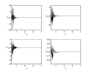
Figure 5: Chaos synchronization: the trajectories of the error dynamical system asymptotically converge to the origin.

Figure 6: The master and the slave system have been synchronized to the chaotic attractor shown in the last subfigure. The parameters of the slave system asymptotically converge to the master system parameter.

In the second numerical test the master systems has been chosen in its hyperchaotic regime, with the parameters $a=36,b=3,c=28,d=-16,k=1$ (the two positive Lyapunov exponents are shown in Fig.1). Let us choose the initial conditions of the master and the slave systems respectively as $\left(x_{m}(0),y_{m}(0),\right.$ $\left.z_{m}(0),w_{m}(0)\right)=(0.3,0.03,0.1,0.2)$ and $\left(x_{s}(0),y_{s}(0),z_{s}(0),\right.$ $\left.w_{s}(0))=(-0.1,0.3,0.01,-0.3\right)$. Given the initial estimated parameters $a_{1}(0)=30,b_{1}(0)=5,$ $c_{1}(0)=25,d_{1}(0)=-20,k_{1}(0)=-1$ and the control gains $(h_{1},h_{2},h_{3},h_{4})=(5,4,6,5)$ the effectiveness of the hyperchaotic synchronization is shown in Figures 7-8.

Figure 7: Hyperchaotic synchronization: the error dynamical system asymptotically converges to the origin.

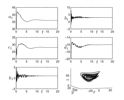
Figure 8: The estimates of the slave system parameters converge to the master system parameters. Both the systems (4.1) and (4.2) evolve to the hyperchaotic attractor shown in the last subfigure.

5 Conclusions

In order to understand the onset of hyperchaotic behavior recently observed in many dynamical systems, we have constructed and analyzed the generalized double Hopf normal form in the modified Chen system which reveals possible regimes of periodic solutions, two-period tori, and three-period tori in parameter space. Numerical simulations are provided showing agreement with the predictions from the normal form. In a future work other possible routes to chaos will be investigated, as further bifurcations of the post-supercritical-Hopf two- and three-tori via either torus doubling or breakdown. Moreover, an adaptive synchronization of the chaotic/hyperchaotic system trajectories has been globally realized and the effectiveness of this control strategy has been numerically illustrated.

References

[1] Austin, F., Sun, W. and Lu, X., Estimation of unknown parameters and adaptive synchronization of hyperchaotic systems, Comm. Nonlinear Sci. Numer. Simulat., 14, pp. 4264-4272 (2009).
[2] Bi, Q. and Yu, P., Double Hopf bifurcations and chaos of a nonlinear vibration system, Nonlinear Dyn., 19, pp. 313-332 (1999).
[3] S. Boccaletti, J. Kurths, G. Osipov, D. Valladares, and C. Zhou, The synchronization
of chaotic systems, Physics Reports, 366, pp. 1 101, (2002).
[4] T. Chen and S. Roy Choudhury, Bifurcations and chaos in a modified driven Chen system,
Far E. J. Dyn. Sys., submitted (2011).
[5] Chen G., Ueta T., Yet another chaotic system, Int.
J. Bifurcat. Chaos, 9, pp. 1465-1466, (1999).
[6]
G. Gambino, S. Roy Choudhury, T. Chen, Modified post-bifurcations dynamics and routes to chaos from double Hopf bifurcations in a hyperchaotic system, accepted for publication, Nonlinear Dynamics (2012).
[7]
G. Gambino, M.C. Lombardo, M. Sammartino, Global linear feedback control for the generalized Lorenz system, Chaos Solitons Fractals, 29,(4), pp. 829-837, (2006).
[8]
G. Gambino, M.C. Lombardo, M. Sammartino, Adaptive control of a seven mode truncation of the Kolmogorov flow with drag, Chaos Solitons Fractals, 41,(1), pp. 47-59, (2009).
[9] T. Gao, Z. Chen, Z. Yuan, and G. Chen, A hyperchaos generated from
Chen s system, International Journal of Modern Physics C, 17, pp. 471
478, (2006).
[10]
Gao T., Gu Q., Chen Z., Analysis of the hyperchaos generated from Chen’s system, Chaos Solitons Fractals, 39, pp. 1849-1855, (2009).
[11] C. Li, X. Liao, and K.-w. Wong, Lag synchronization of hyperchaos with
application to secure communications, Chaos Solitons Fractals, 23,
pp. 183 193, (2005).
[12] C. Li, Q. Chen, and T. Huang, Coexistence of anti-phase and complete
synchronization in coupled Chen system via a single variable, Chaos, Solitons
and Fractals, 38, pp. 461 464, (2008).
[13]
Matsumoto T., Chua, L.O., Kobayasky K., Hyperchaos: laboratory
experiment and numerical confirmation, IEEE Trans. Circ. Syst.,
33, pp. 1143-1147, (1986).
[14]
Nayfeh, A. H., Method of Normal Forms, Wiley, New York, (1993).
[15]
Nayfeh, A. H., Balachandran, Applied Nonlinear Dynamics, Wiley, New York, (1995).
[16] J. H. Park, Adaptive synchronization of hyperchaotic Chen system with uncertain parameters, Chaos, Solitons and Fractals, 26, pp. 959 964, (2005).
[17] L. M. Pecora and T. L. Carroll, Synchronization in chaotic systems, Phys.
Rev. Lett., 64, pp. 821 824, (1990).
[18] M. G. Rosenblum, A. S. Pikovsky, and J. Kurths, Phase synchronization
of chaotic oscillators, Phys. Rev. Lett., 76, pp. 1804 1807, (1996).
[19]
Rössler O. E., An equation for Hyperchaos, Phys. Lett. A,
71, (2-3), pp. 155-157, (1979).
[20]
J. Slotine, W. Li Applied Nonlinear Control, Prentice-Hall, (1991).
[21] H. Xiang and G. Li, A constructional method for generalized synchronization
of coupled time-delay chaotic systems, Chaos, Solitons and Fractals,
41, pp. 1849 1853, (2009).
[22]
Yan Z., Controlling hyperchaos in the new hyperchaotic Chen
system, Appl. Math. Comput., 168, pp. 1239-1250, (2005).
[23]
Yu P., Computation of Normal Forms via a perturbation technique, J. Sound Vibration, 211, pp. 19-38 (1998).
[24]
Yu P., Simplest normal forms of Hopf and generalized Hopf bifurcations, Int. J. Bifurcation and Chaos, 9, pp. 1917-1939 (1999).
[25]
Yu P., Bifurcation, limit cycles and chaos of nonlinear dynamical systems in Bifurcation and Chaos in Complex Systems (Edited Series on Advances in Nonlinear Science and Complexity),
J. Q. Sun and A. C. Luo (Eds.), Elsevier Science & Technology, pp. 1-121, (2006).
[26]
Yu P., Symbolic computation of normal forms for resonant double Hopf bifurcations using a perturbation technique, J. Sound Vibration, 274(4), pp. 615-632 (2001).
[27]
Yu P., Analysis on Double Hopf Bifurcation Using Computer Algebra with the Aid of Multiple Scales, Nonlinear Dyn., 27, pp. 19-53 (2002).
[28]
Wu X., Guan Z., Wu Z., Adaptive synchronization between two different hyperchaotic systems, Nonlinear Analysis, 68, pp. 1346-1351 (2008).
[29] W. Zhu, D. Xu, and Y. Huang, Global impulsive exponential synchronization
of time-delayed coupled chaotic systems, Chaos, Solitons and
Fractals, 35, pp. 904 912, (2008).