Estimation in functional linear quantile regression

Abstract

This paper studies estimation in functional linear quantile regression in which the dependent variable is scalar while the covariate is a function, and the conditional quantile for each fixed quantile index is modeled as a linear functional of the covariate. Here we suppose that covariates are discretely observed and sampling points may differ across subjects, where the number of measurements per subject increases as the sample size. Also, we allow the quantile index to vary over a given subset of the open unit interval, so the slope function is a function of two variables: (typically) time and quantile index. Likewise, the conditional quantile function is a function of the quantile index and the covariate. We consider an estimator for the slope function based on the principal component basis. An estimator for the conditional quantile function is obtained by a plug-in method. Since the so-constructed plug-in estimator not necessarily satisfies the monotonicity constraint with respect to the quantile index, we also consider a class of monotonized estimators for the conditional quantile function. We establish rates of convergence for these estimators under suitable norms, showing that these rates are optimal in a minimax sense under some smoothness assumptions on the covariance kernel of the covariate and the slope function. Empirical choice of the cutoff level is studied by using simulations.

T1Supported by the Grant-in-Aid for Young Scientists (B) (22730179) from the JSPS.

1 Introduction

Quantile regression, initially developed by the seminal work of Koenker and Bassett (1978), is one of the most important statistical methods in measuring the impact of covariates on dependent variables. An attractive feature of quantile regression is that it allows us to make inference on the entire conditional distribution by estimating several different conditional quantiles. Some basic materials on quantile regression and its applications are summarized in Koenker (2005).

This paper studies estimation in functional linear quantile regression in which the dependent variable is scalar while the covariate is a function, and the conditional quantile for each fixed quantile index is modeled as a linear functional of the covariate. The model that we consider is an extension of functional linear regression to the quantile regression case. Here we suppose that covariates are discretely observed and sampling points may differ across subjects, where the number of measurements per subject increases as the sample size. Also, we allow the quantile index to vary over a given subset of the open unit interval, so the slope function is a function of two variables: (typically) time and quantile index. Likewise, the conditional quantile function is a function of the quantile index and the covariate. We consider the problem of estimating the slope function as well as the conditional quantile function itself. The estimator we consider for the slope function is based on the principal component analysis (PCA). Expanding the covariate and the slope function in terms of the PCA basis, the model is transformed into a quantile regression model with an infinite number of regressors. Truncating the infinite sum by the first $m$ (say) terms, we may apply a standard quantile regression technique to estimating the first $m$ coefficients in the basis expansion of the slope function at each quantile index, where $m$ diverges as the sample size. In practice, the population PCA basis is unknown, so it has to be replaced by a suitable estimate for it. Once the estimator for the slope function is available, an estimator for the conditional quantile function is obtained by a plug-in method. Since the so-constructed plug-in estimator not necessarily satisfies the monotonicity constraint with respect to the quantile index, we also consider a class of monotonized estimators for the conditional quantile function.

In summary, we have the following three types of estimators in mind: [(iii)]

a PCA-based estimator for the slope function;

a plug-in estimator for the conditional quantile function;

monotonized estimators for the conditional quantile function. We establish rates of convergence for these estimators under suitable norms, showing that these rates are optimal in a minimax sense under some smoothness assumptions on the covariance kernel of the covariate and the slope function.

In practice, we have to choose the cutoff level empirically. We suggest some criteria, namely, (integrated-)AIC, BIC and GACV, to choose the cutoff level. We study the performance of these criteria by using simulations. In our limited simulation experiments, although none of these criteria clearly dominated the others, (integrated-)BIC worked relatively stably.

Functional data have become increasingly important. For data collected on dense grids, a traditional multivariate analysis is not directly applicable since the number of grid points may be larger than the sample size and the correlation between distinct grid points is potentially high. Functional data analysis views such data as realizations of random functions and takes into account the functional nature of the data. We refer the reader to Ramsay and Silverman (2005) for a comprehensive treatment on functional data analysis. Earlier theoretical studies in functional data analysis have focused on functional linear mean regression models [see Cai and Hall (2006), Cardot, Ferraty and Sarda (1999, 2003), Yao, Müller and Wang (2005), Hall and Horowitz (2007), Crambes, Kneip and Sarda (2009), James, Wang and Zhu (2009), Yuan and Cai (2010), Delaigle and Hall (2012) and references cited in these papers]. Among them, Hall and Horowitz (2007) established fundamental results in functional linear mean regression, deriving sharp rates of convergence for a PCA-based estimator for the slope function under some smoothness assumptions. Note that they assumed that covariates are continuously observed. Other than functional linear mean regression, Müller and Stadtmüller (2005) developed estimation methods for generalized functional linear models using series expansions of covariates and slope functions.

While not many, there are some earlier papers on estimating conditional quantiles with function-valued covariates. Cardot, Crambes and Sarda (2005) studied smoothing splines estimators for functional linear quantile regression models, while their established rates are not sharp. Ferraty, Rabhi and Vieu (2005) considered nonparametric estimation of conditional quantiles when covariates are functions, which is a different topic than ours. Chen and Müller (2012) considered an “indirect” estimation of conditional quantiles. They modeled the conditional distribution as the composition of some (possibly unknown) link function and a linear functional of the covariate. They first estimated the conditional distribution function by adapting the method developed in Müller and Stadtmüller (2005) and then estimated the conditional quantile function by inverting the estimated conditional distribution function. In the quantile regression literature, there are two ways to estimate conditional quantiles. One is to directly model conditional quantiles and estimate unknown parameters by minimizing check functions. The other is to estimate conditional distribution functions and invert them to estimate conditional quantile functions. We refer to the former as a “direct” method while to the latter as an “indirect” method. The approach taken in this paper is classified into a direct method, while that of Chen and Müller (2012) is classified into an indirect method. Note that although their method is flexible, they only established consistency of the estimator.

Conditional quantile estimation offers a variety of fruitful applications for data containing function-valued covariates. A leading example in which conditional quantile estimation with function-valued covariates is useful appears in analysis of growth data [Chen and Müller (2012)]. Suppose that we have a growth data set of girls’ heights between ages $1$ and $18$, say, where multiple measurements may occur at some ages. Use girl’s growth history between ages $1$ and $12$ as a covariate, and her height at age $18$ as a response. Then, conditional quantile estimation gives us an overall picture of the predictive distribution of girl’s height at age $18$ given her growth history between ages $1$ and $12$, which is more informative than just knowing the mean response. In addition to growth data, functional quantile regression has been applied in analysis of ozone pollution data [Cardot, Crambes and Sarda (2007)] and El Niño data [Ferraty, Rabhi and Vieu (2005)]. We believe that functional linear quantile regression modeling is a benchmark modeling in conditional quantile estimation when covariates are functions, just as linear quantile regression modeling is so when covariates are vectors.

Our estimator for the slope function (at a fixed quantile index) can be understood as a regularized solution to an empirical version of a nonlinear ill-posed inverse problem that corresponds to the “normal equation” in the quantile regression case, where the regularization is controlled by the cutoff level. The paper is thus in part related to the literature on statistical nonlinear inverse problems, which is still an ongoing research area [see Bissantz, Hohage and Munk (2004), Horowitz and Lee (2007), Loubes and Ludeña (2010), Chen and Pouzo (2012), Gagliardini and Scaillet (2012)]. On the other hand, in the mean regression case, the normal equation becomes a linear ill-posed inverse problem. Hall and Horowitz (2007) considered two regularized estimators for the slope function based on the normal equation in the mean regression case. Conceptually, the problems handled in our and their papers are different in their nature: linearity and nonlinearity.

From a technical point of view, establishing sharp rates of convergence for our estimators is challenging. Our proof strategy builds upon the techniques developed in the asymptotic analysis for $M$-estimators with diverging numbers of parameters [see, e.g., He and Shao (2000), Belloni, Chernozhukov and Fernández-Val (2011)]. However, the additional complication arises essentially because “regressors” here are estimated ones and the estimation error has to be taken into account, which requires some new techniques such as “conditional” maximal inequalities and some careful moment calculations. Additionally, the discretization error brings a further technical complication.

Finally, the setting here is similar to Section 3 of Crambes, Kneip and Sarda (2009): covariates are densely but discretely observed, and the discretization error is taken into account in the analysis. However, the paper does not cover the case in which covariates are discretely observed with measurement errors because of the technical complication. A formal theoretical analysis in such a case is left to a future work.

The remainder of the paper is organized as follows. Section 2 presents the model and estimators. Section 3 gives the main results in which we derive rates of convergence for the estimators. Section 4 discusses empirical choice of the cutoff level. A proof of Theorem 3.1 is given in Section 5. Some additional discussions, technical proofs, useful technical tools and simulation results are provided in the Appendix. Due to the space limitation, the Appendix is contained in the supplementary file [Kato (2013)].

Throughout the paper, we shall obey the following notation. For $z\in\mathbb{R}^{k}$, let $\|z\|_{\ell^{2}}$ denote the Euclidean norm of $z$. For any integer $k\geq 2$, let $\mathbb{S}^{k-1}$ denote the set of all unit vectors in $\mathbb{R}^{k}$: $\mathbb{S}^{k-1}=\{z\in\mathbb{R}^{p}\dvtx\|z\|_{\ell^{2}}=1\}$. For any $y,z\in\mathbb{R}$, let $y\vee z=\max\{y,z\}$ and $y\wedge z=\min\{y,z\}$. Let $1(\cdot)$ denote the indicator function. For any given (random or nonrandom, scalar or vector) sequence $\{z_{i}\}_{i=1}^{n}$, we use the notation

$$\mathbb{E}_{n}[z_{i}]=\frac{1}{n}\sum_{i=1}^{n}z_{i},$$

which should be distinguished from the population expectation $\mathbb{E}[\cdot]$. For any two sequences of positive constants $r_{n}$ and $s_{n}$, we write $r_{n}\asymp s_{n}$ if the ratio $r_{n}/s_{n}$ is bounded and bounded away from zero. Let $L_{2}[0,1]$ denote the usual $L_{2}$ space with respect to the Lebesgue measure for functions defined on $[0,1]$. Let $\|\cdot\|$ denote the $L_{2}$-norm: $\|f\|^{2}=\int_{0}^{1}f^{2}(t)\,dt$. For any finite set $I$, $\operatorname{Card}(I)$ denotes the cardinality of $I$.

2 Methodology

2.1 Functional linear quantile regression modeling

Let $(Y,X)$ be a pair of a scalar random variable $Y$ and a random function $X=(X(t))_{t\in\mathcal{T}}$ on a bounded closed interval $\mathcal{T}$ in $\mathbb{R}$. Without loss of generality, we assume $\mathcal{T}=[0,1]$. By “random function,” we mean that $X(t)$ is a random variable for each $t\in[0,1]$. For our purpose of formulating a functional linear quantile regression model, we need the existence of the regular conditional distribution of $Y$ given $X$, to which end we assume a mild regularity condition on the path property of $X$. Let $D[0,1]$ denote the space of all càdlàg functions on $[0,1]$, equipped with the Skorohod metric [see Billingsley (1968)]. We assume that the map $t\mapsto X(t)$ is càdlàg almost surely. Equip $D[0,1]$ with the Borel $\sigma$-field. Then, $X$ can be taken as a $D[0,1]$-valued random variable. Since $D[0,1]$ is a Polish space, and the product space $\mathbb{R}\times D[0,1]$ with the product metric is also Polish, the regular conditional distribution of $Y$ given $X$ exists [see, e.g., Dudley (2002), Theorem 10.2.2].

Let $Q_{Y|X}(\cdot|X)$ denote the conditional quantile function of $Y$ given $X$. Let $\mathcal{U}$ be a given subset of $(0,1)$ that is away from $0$ and $1$, that is, for some small $\epsilon\in(0,1/2)$, $\mathcal{U}\subset[\epsilon,1-\epsilon]$. For each $u\in\mathcal{U}$, we assume that $Q_{Y|X}(u|X)$ can be written as a linear functional of $X$, that is, for each $u\in\mathcal{U}$, there exist a scalar constant $a(u)\in\mathbb{R}$ and a scalar function $b(\cdot,u)\in L_{2}[0,1]$ such that

$$Q_{Y|X}(u|X)=a(u)+\int_{0}^{1}b(t,u)X^{c}(t)\,dt,\qquad u\in\mathcal{U},$$ (1)

where $X^{c}(t)=X(t)-\mathbb{E}[X(t)]$. Typical examples of $\mathcal{U}\subset(0,1)$ are as follows: (i) $\mathcal{U}=\{u\}$ (singleton); (ii) $\mathcal{U}=\{u_{1},\ldots,u_{K}\}$ with $0<u_{1}<\cdots<u_{K}<1$ (finite set); (iii) $\mathcal{U}=[u_{L},u_{U}]$ with $0<u_{L}<u_{U}<1$ (bounded closed interval). Formally, we allow for all these possibilities.

The model (1) is a natural extension of standard linear quantile regression models to function-valued covariates and was first formulated in Cardot, Crambes and Sarda (2005). In what follows, we consider estimating the slope function $(t,u)\mapsto b(t,u)$ and the conditional quantile function $(u,x)\mapsto Q_{Y|X}(u|x)$.

Before going to the next step, we briefly give two simple examples of data generating processes that admit the conditional quantile restriction (1).

Example 2.1 ((Linear location design)).

Suppose that $(Y,X)$ obeys the linear location design

$$Y=c+\int_{0}^{1}\varrho(t)X(t)\,dt+\varepsilon,\qquad\varepsilon\mathop{\perp\!\!\!\!\perp}X,$$

where $c$ is a constant and $\varrho(t)$ is a function in $L_{2}[0,1]$. Let $F_{\varepsilon}$ denote the distribution function of $\varepsilon$ and denote by $F_{\varepsilon}^{-1}$ the quantile function of $F_{\varepsilon}$. Then $(Y,X)$ obeys the conditional quantile restriction

$$Q_{Y|X}(u|X)=c+F^{-1}_{\varepsilon}(u)+\int_{0}^{1}\varrho(t)X(t)\,dt,\qquad u\in(0,1).$$

Example 2.2 ((Linear location-scale design)).

Suppose that $(Y,X)$ obeys the linear location-scale design

$$Y=c_{1}+\int_{0}^{1}\varrho_{1}(t)X(t)\,dt+\sigma(X)\varepsilon,\qquad\sigma(X)=c_{2}+\int_{0}^{1}\varrho_{2}(t)X(t)\,dt,\varepsilon\mathop{\perp\!\!\!\!\perp}X,$$

where $c_{1},c_{2}$ are constants and $\varrho_{1}(t),\varrho_{2}(t)$ are functions in $L_{2}[0,1]$. Suppose that $\sigma(X)>0$ almost surely. Denote by $F_{\varepsilon}^{-1}$ the quantile function of the distribution of $\varepsilon$. Then $(Y,X)$ obeys the conditional quantile restriction

$$Q_{Y|X}(u|X)=c_{1}+c_{2}F^{-1}_{\varepsilon}(u)+\int_{0}^{1}\bigl{\{}\varrho_{1}(t)+\varrho_{2}(t)F_{\varepsilon}^{-1}(u)\bigr{\}}X(t)\,dt,\qquad u\in(0,1).$$

In this design, the slope function depends on the quantile index.

2.2 Estimation strategy

We base our estimation strategy on the principal component analysis (PCA). To this end, we additionally assume here that $\int_{0}^{1}\mathbb{E}[X^{2}(t)]\,dt<\infty$. Define the covariance kernel $K(s,t)=\operatorname{Cov}(X(s),\break X(t))$. Then, by the Hilbert–Schmidt theorem, $K(s,t)$ admits the spectral expansion

$$K(s,t)=\sum_{j=1}^{\infty}\kappa_{j}\phi_{j}(s)\phi_{j}(t),$$

where $\kappa_{1}\geq\kappa_{2}\geq\cdots\geq 0$ are ordered eigenvalues, and $\{\phi_{j}\}_{j=1}^{\infty}$ is an orthonormal basis of $L_{2}[0,1]$ consisting of eigenfunctions of the integral operator from $L_{2}[0,1]$ to itself with kernel $K(s,t)$. We will later assume that $\kappa_{j}$ are all positive and there are no ties in $\kappa_{j}$, that is, $\kappa_{1}>\kappa_{2}>\cdots>0$. Since $\{\phi_{j}\}_{j=1}^{\infty}$ is an orthonormal basis of $L_{2}[0,1]$, we have the following expansions in $L_{2}[0,1]$:

$$X^{c}(t)=\sum_{j=1}^{\infty}\xi_{j}\phi_{j}(t),\qquad b(t,u)=\sum_{j=1}^{\infty}b_{j}(u)\phi_{j}(t),$$

where $\xi_{j}$ and $b_{j}(u)$ are defined by

$$\xi_{j}=\int_{0}^{1}X^{c}(t)\phi_{j}(t)\,dt,\qquad b_{j}(u)=\int_{0}^{1}b(t,u)\phi_{j}(t)\,dt.$$

The $\xi_{j}$ are called “principal scores” for $X$. The expansion for $X^{c}$ is called the “Karhunen–Loève expansion.” This leads to the expression $\int_{0}^{1}b(t,u)X^{c}(t)\,dt=\sum_{j=1}^{\infty}b_{j}(u)\xi_{j}$. Then, the model (1) is transformed into a quantile regression model with an infinite number of “regressors”:

$$Q_{Y|X}(u|X)=a(u)+\sum_{j=1}^{\infty}b_{j}(u)\xi_{j},\qquad u\in\mathcal{U}.$$ (2)

Note that $\mathbb{E}[\xi_{j}]=0,\mathbb{E}[\xi_{j}^{2}]=\kappa_{j}$ and $\mathbb{E}[\xi_{j}\xi_{k}]=0$ for all $j\neq k$.

We first consider estimating the slope function $(t,u)\mapsto b(t,u)$. To this end, we estimate the function $b(\cdot,u)$ for each $u\in\mathcal{U}$ and collect them to construct a final estimator for $(t,u)\mapsto b(t,u)$. To explain the basic idea, suppose for a while that (i) $X$ were continuously observable; and (ii) the covariance kernel $K(s,t)$ were known. The problem then reduces to finding suitable estimates of the coefficients $b_{j}(u)$. Let $(Y_{1},X_{1}),\ldots,(Y_{n},X_{n})$ be independent copies of $(Y,X)$. For each $i=1,\ldots,n$, let $\xi_{ij}$ be the principal scores for $X_{i}$. Pick any $u\in\mathcal{U}$. Then, a plausible approach to estimating $b(\cdot,u)$ is to truncate $\sum_{j=1}^{\infty}b_{j}(u)\xi_{j}$ by $\sum_{j=1}^{m}b_{j}(u)\xi_{j}$ for some large $m$, and estimate only the first $m$ coefficients $b_{1}(u),\ldots,b_{m}(u)$ using a standard quantile regression technique. Let $m=m_{n}$ be the “cutoff” level such that $1\leq m\leq n-1$ and $m\to\infty$ as $n\to\infty$. Estimate $a(u)$ and the first $m$ coefficients $b_{1}(u),\ldots,b_{m}(u)$ of $b(\cdot,u)$ by

$$\qquad\bigl{(}\tilde{a}(u),\tilde{b}_{1}(u),\ldots,\tilde{b}_{m}(u)\bigr{)}=\mathop{\arg\min}_{a,b_{1},\ldots,b_{m}}\mathbb{E}_{n}\Biggl{[}\rho_{u}\Biggl{(}Y_{i}-a-\sum_{j=1}^{m}b_{j}\xi_{ij}\Biggr{)}\Biggr{]},$$ (3)

where $\rho_{u}(y)=\{u-1(y\leq 0)\}y$ is the check function [Koenker and Bassett (1978)]. Note that for $u=0.5$, $\rho_{0.5}(\cdot)$ is equivalent to the absolute value function. Here recall that $\mathbb{E}_{n}[z_{i}]=n^{-1}\sum_{i=1}^{n}z_{i}$ for any sequence $\{z_{i}\}_{i=1}^{n}$. The resulting estimator for the slope function $(t,u)\mapsto b(t,u)$ is given by

$$\tilde{b}\dvtx(t,u)\mapsto\tilde{b}(t,u),\qquad\tilde{b}(t,u)=\sum_{j=1}^{m}\tilde{b}_{j}(u)\phi_{j}(t),\qquad t\in[0,1],u\in\mathcal{U}.$$

However, this “estimator” is infeasible since (i) $X$ is usually discretely observed; and (ii) $K(s,t)$ is unknown. Because of (i), it is usually not possible to directly estimate the covariance kernel $K(s,t)$ by the empirical one (since $\mathbb{E}_{n}[(X_{i}(s)-\bar{X}(s))(X_{i}(t)-\bar{X}(t))]$ with $\bar{X}(t)=n^{-1}\sum_{i=1}^{n}X_{i}(t)$ is unavailable for some $(s,t)$). Similarly to Crambes, Kneip and Sarda (2009), we consider the following setting: [(1)]

For each $i=1,\ldots,n$, $X_{i}$ is observed only at $L_{i}+1$ discrete points $0=t_{i1}<t_{i2}<\cdots<t_{i,L_{i}+1}=1$, that is, we only observe $X_{i}(t_{ij}),j=1,\ldots,L_{i}+1$. Typically, $\max_{1\leq i\leq n}\max_{1\leq l\leq L_{i}}(t_{i,l+1}-t_{il})\to 0$ as $n\to\infty$ is assumed.

Based on the discrete observations, for each $i=1,\ldots,n$, construct an interpolated function $\hat{X}_{i}=(\hat{X}_{i}(t))_{t\in[0,1]}$ for $X_{i}=(X_{i}(t))_{t\in[0,1]}$. Here we shall use a simple interpolation rule (see also the later remark):

$$\hat{X}_{i}(t)=\sum_{l=1}^{L_{i}}X(t_{il})1\bigl{(}t\in[t_{il},t_{i,l+1})\bigr{)},\qquad i=1,\ldots,n.$$

The observation time points $t_{i1},\ldots,t_{i,L_{i}+1}$ (and $L_{i}$) should be indexed by the sample size $n$, however, this is suppressed for the notational convenience. Suppose now that the interpolated functions $\hat{X}_{1},\ldots,\hat{X}_{n}$ are obtained. Then, we may estimate the covariance kernel $K(s,t)$ by

$$\hat{K}(s,t)=\mathbb{E}_{n}\bigl{[}\bigl{(}\hat{X}_{i}(s)-\bar{\hat{X}}(s)\bigr{)}\bigl{(}\hat{X}_{i}(t)-\bar{\hat{X}}(t)\bigr{)}\bigr{]},$$

where $\bar{\hat{X}}(t)=n^{-1}\sum_{i=1}^{n}\hat{X}_{i}(t)$. Let $\hat{K}(s,t)=\sum_{j=1}^{\infty}\hat{\kappa}_{j}\hat{\phi}_{j}(s)\hat{\phi}_{j}(t)$ be the spectral expansion of $\hat{K}(s,t)$, where $\hat{\kappa}_{1}\geq\hat{\kappa}_{2}\geq\cdots\geq 0$ are ordered eigenvalues and $\{\hat{\phi}_{j}\}_{j=1}^{\infty}$ is an orthonormal basis of $L_{2}[0,1]$ consisting of eigenfunctions of the integral operator from $L_{2}[0,1]$ to itself with kernel $\hat{K}(s,t)$. Each principal score $\xi_{ij}$ is now estimated by

$$\hat{\xi}_{ij}=\int_{0}^{1}\bigl{(}\hat{X}_{i}(t)-\bar{\hat{X}}(t)\bigr{)}\hat{\phi}_{j}(t)\,dt.$$

Then, the coefficients $a(u)$ and $b_{1}(u),\ldots,b_{m}(u)$ are estimated by

$$\quad\bigl{(}\hat{a}(u),\hat{b}_{1}(u),\ldots,\hat{b}_{m}(u)\bigr{)}=\mathop{\arg\min}_{a,b_{1},\ldots,b_{m}}\mathbb{E}_{n}\Biggl{[}\rho_{u}\Biggl{(}Y_{i}-a-\sum_{j=1}^{m}b_{j}\hat{\xi}_{ij}\Biggr{)}\Biggr{]}.$$ (4)

The resulting estimator for the slope function $(t,u)\mapsto b(t,u)$ is given by

$$\hat{b}\dvtx(t,u)\mapsto\hat{b}(t,u),\qquad\hat{b}(t,u)=\sum_{j=1}^{m}\hat{b}_{j}(u)\hat{\phi}_{j}(t),\qquad t\in[0,1],u\in\mathcal{U}.$$

The optimization problem (4) can be transformed into a linear programming problem and can be solved by using standard statistical softwares. Once the estimator for the slope function is obtained, the conditional $u$-quantile of $Y$ given $X=x$ for a given function $x=(x(t))_{t\in[0,1]}\in L_{2}[0,1]$ is estimated by a plug-in method:

$$\hat{Q}_{Y|X}(u|x)=\hat{a}(u)+\int_{0}^{1}\hat{b}(t,u)\bigl{(}x(t)-\bar{\hat{X}}(t)\bigr{)}\,dt.$$

Empirical choice of the cutoff level will be discussed in Section 4.

The basis $\{\phi_{j}\}_{j=1}^{\infty}$ is called the (population) PCA basis. Alternatively, one may use other basis functions independent of the data, such as Fourier and wavelet bases, in which case the analysis becomes more tractable. A potential drawback of using such basis functions is that, as discussed in Delaigle and Hall (2012), using the “first” $m$ basis functions is less motivated. The PCA basis is a benchmark basis in functional data analysis, which is the reason why the PCA basis is used in this paper. Other estimation methods such as smoothing splines [Crambes, Kneip and Sarda (2009)] and a reproducing kernel Hilbert space approach [Yuan and Cai (2010)] could be adapted in the quantile regression case, which is left as a future topic.

The interpolation rule used here may be replaced by any other reasonable interpolation rule. For example, a plausible alternative is to use

$$\hat{X}_{i}^{\mathrm{mid}}(t)=\sum_{l=1}^{L_{i}}\frac{X(t_{il})+X(t_{i,l+1})}{2}1\bigl{(}t\in[t_{il},t_{i,l+1})\bigr{)},\qquad i=1,\ldots,n.$$

It is not hard to see that the theory below also applies to this interpolation rule. In practice, this interpolation rule may be more recommended since it uses all the discrete observations $X_{i}(t_{i1}),\ldots,X_{i}(t_{i,L_{i}+1})$.

Finally, we note that for any fixed $u\in\mathcal{U}$, our estimator $\hat{b}(\cdot,u)$ can be understood as a regularized solution to an empirical version of a nonlinear ill-posed inverse problem that corresponds to the “normal equation” in the quantile regression case. Due to the space limitation, we shall discuss this connection to nonlinear ill-posed inverse problems in Appendix A in the supplementary file [Kato (2013)].

2.3 Monotonization

Suppose in this section that $\mathcal{U}$ is a bounded closed interval: $\mathcal{U}=[u_{L},u_{U}]$ with $0<u_{L}<u_{U}<1$. The conditional quantile function $Q_{Y|X}(u|x)$ is monotonically nondecreasing in $u$. However, the plug-in estimator $\hat{Q}_{Y|X}(u|x)$ constructed is not necessarily so. To circumvent this problem, we may monotonize the map $u\mapsto\hat{Q}_{Y|X}(u|x)$ by one of the following three methods: (i) rearrangement [Chernozhukov, Fernández-Val and Galichon (2009)], (ii) isotonization [Barlow et al. (1972)], (iii) convex combination of (i) and (ii). Such methods are explained in Chernozhukov, Fernández-Val and Galichon (2009) in a general setup. We briefly explain their basic ideas. Pick any $x\in L_{2}[0,1]$.

[(iii)]

Rearrangement. Define the function

$$\hat{F}_{\mathcal{U}}(y|x)=\frac{1}{u_{U}-u_{L}}\int_{\mathcal{U}}1\bigl{\{}\hat{Q}_{Y|X}(u|x)\leq y\bigr{\}}\,du.$$

Then the map $y\mapsto\hat{F}_{\mathcal{U}}(y|x)$ is a proper distribution function supported in $[\min_{u\in\mathcal{U}}\hat{Q}_{Y|X}(u|x),\max_{u\in\mathcal{U}}\hat{Q}_{Y|X}(u|x)]$. The rearranged estimator for$Q_{Y|X}(u|x)$ is defined by

$$\hat{Q}^{*}_{Y|X}(u|x)=\hat{F}^{-1}_{\mathcal{U}}\biggl{(}\frac{u-u_{L}}{u_{U}-u_{L}}\Big{|}x\biggr{)}.$$

Clearly, the map $u\mapsto\hat{Q}_{Y|X}^{*}(u|x)$ is nondecreasing.

Isotonization. The isotonization is carried out by projecting the original estimate $u\mapsto\hat{Q}_{Y|X}(u|x)$ on the set of nondecreasing functions, typically by the “pool adjacent violators” algorithm. Denote by $\hat{Q}^{I}_{Y|X}(u|x)$ the isotonized estimator.

Convex combination of (i) and (ii). Take $\lambda\in[0,1]$. Then, the convex combination $\hat{Q}^{\lambda}_{Y|X}(u|x)=\lambda\hat{Q}^{*}_{Y|X}(u|x)+(1-\lambda)\hat{Q}_{Y|X}^{I}(u|x)$ is nondecreasing in $u$.

By Chernozhukov, Fernández-Val and Galichon (2009), it is shown that any monotonized estimate [constructed by using one of (i)–(iii)] is at least as good as the initial estimate $\hat{Q}_{Y|X}(u|x)$ in the following sense: let $\hat{Q}^{\dagger}_{Y|X}(u|x)$ be any monotonized estimate for $Q_{Y|X}(u|x)$ given above. Then, we have for all $q\in[1,\infty]$,

$$\biggl{[}\int_{\mathcal{U}}\bigl{|}\hat{Q}^{\dagger}_{Y|X}(u|x)-Q_{Y|X}(u|x)\bigr{|}^{q}\,du\biggr{]}^{1/q}$$

(5)

$$\qquad\leq\biggl{[}\int_{\mathcal{U}}\bigl{|}\hat{Q}_{Y|X}(u|x)-Q_{Y|X}(u|x)\bigr{|}^{q}\,du\biggr{]}^{1/q},$$

where the obvious modification is made when $q=\infty$.

3 Rates of convergence

In this section we derive rates of convergence for the estimators defined in the previous section and argue their optimality. We make the following assumptions. Let $C_{1}>1$ be some sufficiently large constant. First of all, we assume the following:

[(A1)]

$\{(Y_{i},X_{i})\}_{i=1}^{\infty}$ is i.i.d. with $(Y,X)$.

$\int_{0}^{1}\mathbb{E}[X^{4}(t)]\,dt\leq C_{1}$ and $\mathbb{E}[\xi_{j}^{4}]\leq C_{1}\kappa_{j}^{2}$ for all $j\geq 1$.

The i.i.d. assumption is conventional. It is beyond the scope of the paper to extend the theory to dependent data. Note that Hörmann and Kokoszka (2010) discussed weakly dependent functional data. Assumption (A2) is a mild moment restriction. Here no moment condition on $Y$ is needed, so $\mathbb{E}[Y]$ may not exist.

[(A3)]

For some $\alpha>1$, $C_{1}^{-1}j^{-\alpha}\leq\kappa_{j}\leq C_{1}j^{-\alpha}$ and $\kappa_{j}-\kappa_{j+1}\geq C_{1}^{-1}j^{-\alpha-1}$ for all $j\geq 1$.

For some $\beta>\alpha/2+1$, $\sup_{u\in\mathcal{U}}|b_{j}(u)|\leq C_{1}j^{-\beta}$ for all $j\geq 1$.

Let $F_{Y|X}(y|X)$ denote the conditional distribution function of $Y$ given $X$. Then, for every realization of $X$, the map $y\mapsto F_{Y|X}(y|X)$ is twice continuously differentiable with $f_{Y|X}(y|X)=\partial F_{Y|X}(y|X)/\partial y$ and$f^{\prime}_{Y|X}(y|X)=\partial f_{Y|X}(y|X)/\partial y$. Furthermore, $f_{Y|X}(y|X)\vee|f_{Y|X}^{\prime}(y|X)|\leq C_{1}$.

$\inf_{u\in\mathcal{U}}f_{Y|X}(Q_{Y|X}(u|X)|X)\geq C_{1}^{-1}$.

Assumptions (A3) and (A4) are adapted from (3.2) and (3.3) of Hall and Horowitz (2007). Assumption (A3) especially means that all $\kappa_{j}$ are positive, which guarantees identification of the slope function. In assumption (A3), $\alpha$ measures the smoothness of the covariance kernel $K$, which also measures the difficulty of estimating the slope function $(t,u)\mapsto b(t,u)$. The second part of assumption (A3) is to require the spacings among $\kappa_{j}$ not be too small, which ensures identifiability of eigenfunctions $\phi_{j}$ and thereby sufficient estimation accuracy of $\hat{\phi}_{j}$. Note that the lower inequality for $\kappa_{j}$ follows essentially from the condition on the difference, as $\kappa_{j}\to 0$ ($j\to\infty$) and hence $\kappa_{j}=\sum_{k=j}^{\infty}(\kappa_{k}-\kappa_{k+1})$. Assumption (A4) determines the “smoothness” of the function $t\mapsto b(t,u)$. The condition that $\beta>\alpha/2+1$ requires the function $t\mapsto b(t,u)$ to be sufficiently smooth relative to $K$ uniformly in $u\in\mathcal{U}$. See Hall and Horowitz [(2007), page 74] for some related discussions on these assumptions. Assumptions (A5) and (A6) are specific to the quantile regression case. Both assumptions are standard in the quantile regression literature when $X$ is a vector. The role of assumption (A6) is to guarantee that the conditional distribution function $F_{Y|X}(y|X)$ is not “flat” near quantiles of interest, which is essential to our asymptotic study.

[(A7)]

For each $i=1,\ldots,n$, $X_{i}$ is observed only at discrete points $0=t_{i1}<t_{i2}<\cdots<t_{i,L_{i}+1}=1$. Define $\Delta=\Delta_{n}=\max_{1\leq i\leq n}\max_{1\leq l\leq L_{i}}(t_{i,l+1}-t_{il})$. Then, $\Delta\to 0$ as $n\to\infty$.

There exists a constant $\gamma\in(0,2]$ such that $\mathbb{E}[(X(t)-X(s))^{2}]\leq C_{1}|t-s|^{\gamma}$ for all $s,t\in[0,1]$.

Assumptions (A7) and (A8) are a set of sampling assumptions on $X_{i}$. A rate restriction will be imposed on $\Delta$. Assumption (A7) at least requires that $\min_{1\leq i\leq n}L_{i}\to\infty$ as $n\to\infty$, which means that each set of discrete points $t_{i1},\ldots,t_{i,L_{i}+1}$ has to be dense in $[0,1]$ as the sample size grows. Assumption (A8) is an additional assumption on the smoothness of the covariance kernel as well as the mean function $t\mapsto\mathbb{E}[X(t)]$. Suppose in this discussion $\mathbb{E}[X(t)]=0$ for all $t\in[0,1]$. Then, for example, $\gamma=1$ if $K(s,t)$ is Lipschitz continuous and $\gamma=2$ if $K(s,t)$ is twice continuously differentiable. The value of $\gamma$ controls the discretization error. Note that possible values of $\gamma$ depend on the value of $\alpha$. Typically, if $\alpha$ is sufficiently large, (A8) is satisfied with $\gamma=2$ (and vice versa). The relation between the smoothness of the covariance (or more generally integral) kernel and the decay rate of the associated eigenvalues is studied in Ritter, Wasilkowski and Woźniakowski (1995) and Ferreira and Menegatto (2009) and the references therein. For example, the former paper shows that, if $K$ verifies the “Sacks–Ylvisaker condition” of order $r$ with $r$ a nonnegative integer (see the original paper for the precise description of the conditions), in which case (A8) is satisfied with $\gamma=2$, then $\kappa_{j}\asymp j^{-2r-2}$ as $j\to\infty$. Assumption (A8) is similar in spirit to (A2) of Crambes, Kneip and Sarda (2009), in which they directly assumed some smoothness of the random function $t\mapsto X(t)$ to deal with the discretization error [roughly speaking, their $2\kappa$ corresponds to our $\gamma$ as (A2) of Crambes, Kneip and Sarda (2009) essentially assumes $X$ to be $\kappa$-Hölder continuous and in that case $\mathbb{E}[(X(t)-X(s))^{2}]=O(|t-s|^{2\kappa})$].

Let $\mathcal{F}=\mathcal{F}(C_{1},\alpha,\beta,\gamma)$ denote the set of all distributions of $(Y,X)$ compatible with assumptions (A2)–(A6) and (A8) for given (admissible) values of $C_{1},\alpha,\beta$ and $\gamma$ (such that $\mathcal{F}\neq\varnothing$). The following theorem, which will be proved in Section 5 below, establishes rates of convergence for the slope estimator $(t,u)\mapsto\hat{b}(t,u)$.

Theorem 3.1

Suppose that assumptions (A1)–(A8) are satisfied. Take $m=m_{n}\asymp n^{1/(\alpha+2\beta)}$. Then, we have

$$\lim_{M\to\infty}\limsup_{n\to\infty}\sup_{F\in\mathcal{F}}\mathbb{P}_{F}\biggl{[}\sup_{u\in\mathcal{U}}\int_{0}^{1}\bigl{\{}\hat{b}(t,u)-b(t,u)\bigr{\}}^{2}\,dt$$

(6)

$$\hskip 135.0pt{}>Mn^{-(2\beta-1)/(\alpha+2\beta)}\biggr{]}=0,$$

provided that $(n\vee(\log n)m^{3\alpha+3})\Delta^{\gamma}=O(1)$ as $n\to\infty$.

Inspection of the proof of Theorem 3.1 shows that, when $X$ is continuously observable, under assumptions (A1)–(A6), the rate of convergence of the estimator based on the direct empirical covariance kernel will be $n^{-(2\beta-1)/(\alpha+2\beta)}$. The side condition that $(n\vee(\log n)m^{3\alpha+3})\Delta^{\gamma}=O(1)$ is assumed to make the discretization error negligible. This condition seems not quite restrictive. For example, if $\beta\geq\alpha+3/2$ and $\gamma=2$, it is satisfied as long as $\Delta=O((n\log n)^{-1/2})$, which seems to be mild in view of some applications in functional data analysis.

The following theorem, which will be proved in Appendix B in the supplementary file [Kato (2013)], establishes rates of convergence for $\hat{Q}_{Y|X}(u|x)$. For notational convenience, define

$$\mathcal{E}(\hat{Q}_{Y|X},u)=\int\bigl{\{}\hat{Q}_{Y|X}(u|x)-Q_{Y|X}(u|x)\bigr{\}}^{2}\,dP_{X}(x),$$

where $P_{X}$ denotes the distribution of $X$ (defined on $D[0,1]$).

Theorem 3.2

Suppose that assumptions (A1)–(A8) are satisfied. Take $m=m_{n}\asymp n^{1/(\alpha+2\beta)}$. Then, we have

$$\lim_{M\to\infty}\limsup_{n\to\infty}\sup_{F\in\mathcal{F}}\mathbb{P}_{F}\Bigl{[}\sup_{u\in\mathcal{U}}\mathcal{E}(\hat{Q}_{Y|X},u)>Mn^{-(\alpha+2\beta-1)/(\alpha+2\beta)}\Bigr{]}=0,$$ (7)

provided that $(n\vee(\log n)m^{3\alpha+3})\Delta^{\gamma}=O(1)$ as $n\to\infty$.

For monotonized estimators, the following corollary directly follows in view of (2.3) and Theorem 3.2.

Corollary 3.1

Let $\mathcal{U}$ be a bounded closed interval in $(0,1)$. Suppose that all the assumptions of Theorem 3.2 are satisfied. Let $\hat{Q}^{\dagger}_{Y|X}(u|x)$ be any monotonized estimator for $Q_{Y|X}(u|x)$ given in Section 2.3. Then, we have

$$\lim_{M\to\infty}\limsup_{n\to\infty}\sup_{F\in\mathcal{F}}\mathbb{P}_{F}\biggl{[}\int_{\mathcal{U}}\mathcal{E}\bigl{(}\hat{Q}^{\dagger}_{Y|X},u\bigr{)}\,du>Mn^{-(\alpha+2\beta-1)/(\alpha+2\beta)}\biggr{]}=0.$$

Here note that the rate $n^{-(\alpha+2\beta-1)/(\alpha+2\beta)}$ attained in estimating $Q_{Y|X}(u|x)$ is faster than the rate $n^{-(2\beta-1)/(\alpha+2\beta)}$ attained in estimating $b(t,u)$.

In what follows, we discuss optimality of these rates.

Proposition 3.1

Suppose that assumptions (A1)–(A6) and (A8) are satisfied. Let $\gamma$ be such that

$$0<\gamma\cases{<\alpha-1,&\quad$\mbox{if $\alpha\leq 3$},$\vspace*{2pt}\cr\leq 2,&\quad$\mbox{if $\alpha>3$}.$}$$ (8)

Then, there exists a constant $M>0$ such that for $\mathcal{F}=\mathcal{F}(C_{1},\alpha,\beta,\gamma)$,

$$\liminf_{n\to\infty}\inf_{\bar{b}}\sup_{F\in\mathcal{F}}\mathbb{P}_{F}\biggl{[}\sup_{u\in\mathcal{U}}\int_{0}^{1}\bigl{\{}\bar{b}(t,u)-b(t,u)\bigr{\}}^{2}\,dt$$

(9)

$$\hskip 118.0pt{}>Mn^{-(2\beta-1)/(\alpha+2\beta)}\biggr{]}>0,$$

where $\inf_{\bar{b}}$ is taken over all estimators for the slope function $(t,u)\mapsto b(t,u)$ based on $(Y_{1},X_{1}),\ldots,(Y_{n},X_{n})$. Similarly, there exists a constant $M>0$ such that for $\mathcal{F}=\mathcal{F}(C_{1},\alpha,\beta,\gamma)$,

$$\liminf_{n\to\infty}\inf_{\bar{Q}_{Y|X}}\sup_{F\in\mathcal{F}}\mathbb{P}_{F}\Bigl{[}\sup_{u\in\mathcal{U}}\mathcal{E}(\bar{Q}_{Y|X},u)>Mn^{-(\alpha+2\beta-1)/(\alpha+2\beta)}\Bigr{]}>0,$$

where $\inf_{\bar{Q}_{Y|X}}$ is taken over all estimators for the conditional quantile function $Q_{Y|X}\dvtx(u,x)\mapsto Q_{Y|X}(u|x)$ based on $(Y_{1},X_{1}),\ldots,(Y_{n},X_{n})$. When $\mathcal{U}$ is a bounded closed interval in $(0,1)$, there exists a constant $M>0$ such that for $\mathcal{F}=\mathcal{F}(C_{1},\alpha,\beta,\gamma)$,

$$\liminf_{n\to\infty}\inf_{\bar{Q}_{Y|X}}\sup_{F\in\mathcal{F}}\mathbb{P}_{F}\biggl{[}\int_{\mathcal{U}}\mathcal{E}(\bar{Q}_{Y|X},u)\,du>Mn^{-(\alpha+2\beta-1)/(\alpha+2\beta)}\biggr{]}>0,$$

where the previous convention applies.

The side condition (8) is a compatibility condition between assumptions (A3) and (A8). It is not addressed here whether this condition is tight. However, some restriction between $\alpha$ and $\gamma$ is required in establishing lower bounds of rates of convergence to guarantee that the class $\mathcal{F}(C_{1},\alpha,\beta,\gamma)$ is at least nonempty. Proposition 3.1 shows that under this side condition the rates established in Theorems 3.1, 3.2 and Corollary 3.1 are indeed optimal in the minimax sense. A proof of Proposition 3.1 is given in Appendix C in the supplementary file [Kato (2013)].

4 Empirical choice of the cutoff level

In this section we suggest three criteria to choose $m$, and investigate their performance by simulations. We use a heuristic reasoning to derive selection criteria. Suppose that $\mathcal{U}$ is a singleton: $\mathcal{U}=\{u\}$. Suppose that there is no truncation bias, that is, $b(t,u)=\sum_{j=1}^{m}b_{j}(u)\phi_{j}(t)$ and $Q_{Y|X}(u|X)=a(u)+\sum_{j=1}^{m}b_{j}(u)\xi_{j}$. Then, the infeasible estimator $(\tilde{a}(u),\tilde{b}_{1}(u),\ldots,\tilde{b}_{m}(u))^{\prime}$ defined by (3) can be regarded as a (conditional) maximum likelihood estimator when the conditional distribution of $Y$ given $X$ has the asymmetric Laplace density of the form

$$f(y|X,u,\sigma)=\frac{u(1-u)}{\sigma}\exp\Biggl{\{}-\frac{1}{\sigma}\rho_{u}\Biggl{(}y-a(u)-\sum_{j=1}^{m}b_{j}(u)\xi_{j}\Biggr{)}\Biggr{\}},$$

where $\sigma>0$ is a scale parameter. This suggests the following analogues of AIC and BIC in the present context:

$$\mathtt{AIC}(u) = \log\Biggl{[}\frac{1}{n}\sum_{i=1}^{n}\rho_{u}\Biggl{(}Y_{i}-\hat{a}(u)-\sum_{j=1}^{m}\hat{b}_{j}(u)\hat{\xi}_{ij}\Biggr{)}\Biggr{]}+\frac{(m+1)}{n},$$

$$\mathtt{BIC}(u) = \log\Biggl{[}\frac{1}{n}\sum_{i=1}^{n}\rho_{u}\Biggl{(}Y_{i}-\hat{a}(u)-\sum_{j=1}^{m}\hat{b}_{j}(u)\hat{\xi}_{ij}\Biggr{)}\Biggr{]}+\frac{(m+1)\log n}{n}.$$

See also Koenker [(2005), Section 4.9.1] for some related discussion. According to Yuan (2006), we may also consider an analogue of GACV as follows:

$$\mathtt{GACV}(u)=\frac{\sum_{i=1}^{n}\rho_{u}(Y_{i}-\hat{a}(u)-\sum_{j=1}^{m}\hat{b}_{j}(u)\hat{\xi}_{ij})}{n-(m+1)}.$$

When $\mathcal{U}$ is a bounded closed interval, define the integrated-AIC, BIC and GACV as follows:

$$\mathtt{IAIC} = \int_{\mathcal{U}}\mathtt{AIC}(u)\,du,\qquad\mathtt{IBIC}=\int_{\mathcal{U}}\mathtt{BIC}(u)\,du,$$

$$\mathtt{IGACV} = \int_{\mathcal{U}}\mathtt{GACV}(u)\,du.$$

When $\mathcal{U}$ is a set of finite grid points, each integral is replaced by the summation over the grid points.

We carried out a small Monte Carlo study to investigate the finite sample performance of these criteria. In all cases, the number of Monte Carlo repetitions was $1000$. The numerical results obtained in this section were carried out by using the matrix language Ox [Doornik (2002)]. The Ox code for solving quantile regression problems supplied on Professor Koenker’s website was used. See also Portnoy and Koenker (1997) for some computational aspects of quantile regression problems.

The simulation design is described as follows:

$$Y = \int_{0}^{1}\varrho(t)X(t)\,dt+\varepsilon,$$

$$\varrho(t) = \sum_{j=1}^{50}\varrho_{j}\phi_{j}(t),$$

$$\eqntext{\varrho_{1}=0.3,\varrho_{j}=4(-1)^{j+1}j^{-2},j\geq 2,\phi_{j}(t)=2^{1/2}\cos(j\pi t),}$$ (10)

$$X(t) = \sum_{j=1}^{50}\gamma_{j}Z_{j}\phi_{j}(t),$$

$$\eqntext{\gamma_{j}=(-1)^{j+1}j^{-\alpha/2},\alpha\in\{1.1,2\},Z_{j}\sim U\bigl{[}-3^{1/2},3^{1/2}\bigr{]},}$$ (11)

$$\varepsilon \sim N(0,1)\mbox{ or }\mbox{Cauchy},\qquad n\in\{100,200,500\}.$$

This $\alpha$ corresponds to $\alpha$ in assumption (A3). Each $X_{i}$ is observed at $201$ equally spaced grid points on $[0,1]$. In this design, we have

$$Q_{Y|X}(u|X)=F_{\varepsilon}^{-1}(u)+\int_{0}^{1}\varrho(t)X(t)\,dt,$$

where $F_{\varepsilon}^{-1}(\cdot)$ is the quantile function of the distribution of $\varepsilon$. Thus, $a(u)=F_{\varepsilon}^{-1}(u)$ and $b(t,u)\equiv\varrho(t)$ [$b(t,u)$ is independent of $u$]. We considered two cases for $\mathcal{U}$: (a) $\mathcal{U}=\{0.5\}$ and (b) $\mathcal{U}=\{0.15,0.2,\ldots,0.85\}$. In each case, the performance was measured by

$$\mathtt{QA\mbox{-}MISE} = \frac{1}{\operatorname{Card}(\mathcal{U})}\sum_{u\in\mathcal{U}}\mathbb{E}\biggl{[}\int_{0}^{1}\bigl{\{}\hat{b}(t,u)-b(t,u)\bigr{\}}^{2}\,dt\biggr{]}\quad\mbox{or}$$

$$\mathtt{QA\mbox{-}MISE} = \frac{1}{\operatorname{Card}(\mathcal{U})}\sum_{u\in\mathcal{U}}\mathbb{E}\biggl{[}\int\bigl{\{}\hat{Q}_{Y|X}(u|x)-Q_{Y|X}(u|x)\bigr{\}}^{2}\,dP_{X}(x)\biggr{]},$$

where $P_{X}$ denotes the distribution of $X$ and $\mathtt{QA\mbox{-}MISE}$ is the abbreviation of “quantile-averaged mean integrated squared error.”

The simulation results for case (a) are summarized in Figures 1–4 and Table 1. Figures 1 and 2 show the performance of the selection criteria for the normal error case, while Figures 3 and 4 show that for the Cauchy error case. In each figure, “Fixed” refers to the performance of the estimator with fixed $m$. Table 1 shows the average numbers of $m$ selected by three criteria. The table shows that as the sample size increases, all the criteria tend to choose larger $m$, and as $\alpha$ increases, they tend to choose smaller $m$, which is consistent with the theoretical requirement in the $m$-selection. Interestingly, it is observed that the error distribution affects the performance of the $m$-selection.

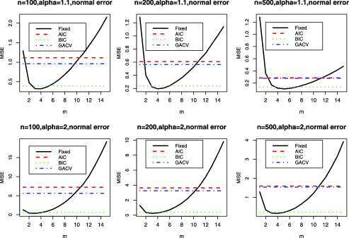
Figure 1: Performance of selection criteria. Case (a). Estimation of $b(\cdot,0.5)$.

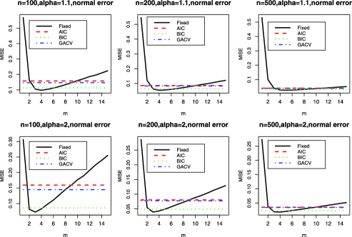
Figure 2: Performance of selection criteria. Case (a). Estimation of $Q_{Y|X}(0.5|x)$.

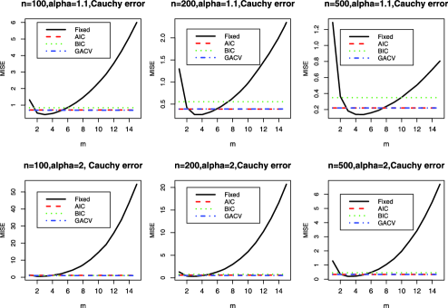
Figure 3: Performance of selection criteria. Case (a). Estimation of $b(\cdot,0.5)$.

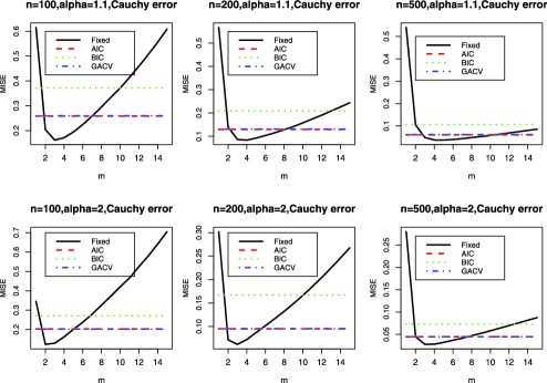
Figure 4: Performance of selection criteria. Case (a). Estimation of $Q_{Y|X}(0.5|x)$.

In the normal error case, in Figure 1, BIC worked better than the other two criteria. On the other hand, in the Cauchy error case, in Figure 2, AIC and GACV worked better than BIC. Looking closely at these figures, one finds that AIC and GACV performed quite badly in some cases (see the bottom half in Figure 1). Although none of these criteria clearly dominated the others, BIC worked relatively stably. These figures also show that as $\alpha$ increases from $1.1$ to $2$, the performance of $\hat{b}(\cdot,0.5)$ becomes worse, while that of $\hat{Q}_{Y|X}(0.5|x)$ becomes better. This is consistent with the theoretical results in the previous section. Essentially similar comments apply to case (b), Figures 1–4 and Table 1 in Appendix F in the supplementary file [Kato (2013)].

Table 1: Average numbers of $m$ selected by three criteria in case (a). Standard deviations are given in parentheses

$\bolds{n}$	$\bolds{\alpha}$	error dist.	AIC	BIC	GACV
100	1.1	normal	7.40 (4.12)	3.09 (1.24)	6.58 (3.78)
200	1.1	normal	7.34 (3.87)	3.39 (1.14)	6.98 (3.67)
500	1.1	normal	8.13 (3.59)	3.94 (1.05)	7.97 (3.52)
100	20.	normal	6.50 (4.23)	2.53 (0.93)	5.67 (3.84)
200	20.	normal	6.33 (3.95)	2.67 (0.85)	5.96 (3.76)
500	20.	normal	6.92 (3.85)	3.12 (0.77)	6.81 (3.80)
100	1.1	Cauchy	2.30 (1.18)	1.62 (0.61)	2.24 (1.08)
200	1.1	Cauchy	2.51 (0.88)	1.91 (0.64)	2.48 (0.84)
500	1.1	Cauchy	3.00 (0.87)	2.20 (0.51)	2.99 (0.86)
100	20.	Cauchy	1.90 (0.94)	1.35 (0.51)	1.86 (0.81)
200	20.	Cauchy	2.14 (0.76)	1.60 (0.53)	2.10 (0.60)
500	20.	Cauchy	2.41 (0.67)	1.91 (0.38)	2.40 (0.67)

5 Proof of Theorem 3.1

We divide the proof into three subsections. Some technical results are proved in Appendices D and E in the supplementary file [Kato (2013)]. To avoid the notational complication, uniformity in $F\in\mathcal{F}$ will be suppressed. Let $C>0$ denote a generic constant of which the value may change from line to line. In most cases, qualification “almost surely” will be suppressed. In some parts of the proofs, we use empirical process techniques. We follow the basic notation used in van der Vaart and Wellner (1996).

5.1 Reduction of the problem

Let $b_{0}(u)=a(u),\hat{b}_{0}(u)=\hat{a}(u)$ and $\xi_{i0}=\hat{\xi}_{i0}=1$. For any $v_{0},\ldots,v_{m}\in\mathbb{R}$, write $v^{m}=(v_{0},\ldots,v_{m})^{\prime}$. For $v^{m}\in\mathbb{R}^{m+1}$ and $w^{m}\in\mathbb{R}^{m+1}$, write $v^{m}\cdot w^{m}=\sum_{j=0}^{m}v_{j}w_{j}$. Then,

$$\hat{b}^{m}(u)=\bigl{(}\hat{b}_{0}(u),\hat{b}_{1}(u),\ldots,\hat{b}_{m}(u)\bigr{)}^{\prime}=\mathop{\arg\min}_{b^{m}\in\mathbb{R}^{m+1}}\mathbb{E}_{n}\bigl{[}\rho_{u}\bigl{(}Y_{i}-\hat{\xi}_{i}^{m}\cdot b^{m}\bigr{)}\bigr{]}.$$

We use a further re-parameterization. For $i=1,\ldots,n$ and $j\geq 1$, let $\eta_{ij}=\kappa_{j}^{-1/2}\xi_{ij},\hat{\eta}_{ij}=\kappa_{j}^{-1/2}\hat{\xi}_{ij},d_{j}(u)=\kappa_{j}^{1/2}b_{j}(u)$ and $\hat{d}_{j}(u)=\kappa_{j}^{1/2}\hat{b}_{j}(u)$. For $j=0$, define $\eta_{i0}=\hat{\eta}_{i0}=1$, $d_{0}(u)=b_{0}(u)$ and $\hat{d}_{0}(u)=\hat{b}_{0}(u)$. Note that $\mathbb{E}[\eta_{ij}]=0,\mathbb{E}[\eta_{ij}^{2}]=1$ for all $j\geq 1$, and $\mathbb{E}[\eta_{ij}\eta_{ik}]=0$ for all $j,k\geq 0$ with $j\neq k$. Then,

$$\hat{d}^{m}(u)=\bigl{(}\hat{d}_{0}(u),\hat{d}_{1}(u),\ldots,\hat{d}_{m}(u)\bigr{)}^{\prime}=\mathop{\arg\min}_{d^{m}\in\mathbb{R}^{m+1}}\mathbb{E}_{n}\bigl{[}\rho_{u}\bigl{(}Y_{i}-\hat{\eta}_{i}^{m}\cdot d^{m}\bigr{)}\bigr{]}.$$

We first consider bounding $\sup_{u\in\mathcal{U}}\|\hat{d}^{m}(u)-d^{m}(u)\|_{\ell^{2}}$.

Lemma 5.1

Suppose that for all $\epsilon>0$, there exist constants $c>0$ and $M>0$ possibly depending on $\epsilon$ such that

$$\liminf_{n\to\infty}\mathbb{P}\bigl{\{}-\mathbb{E}_{n}\bigl{[}\bigl{\{}u-1\bigl{(}Y_{i}\leq\hat{\eta}_{i}^{m}\cdot\bigl{(}d^{m}(u)+M\sqrt{m/n}h^{m}\bigr{)}\bigr{)}\bigr{\}}\bigl{(}h^{m}\cdot\hat{\eta}_{i}^{m}\bigr{)}\bigr{]}$$

$$\hskip 147.0pt\qquad>c\sqrt{m/n}\ \forall u\in\mathcal{U},\forall h^{m}\in\mathbb{S}^{m}\bigr{\}}>1-\epsilon.$$

Then, we have

$$\limsup_{n\to\infty}\mathbb{P}\Bigl{\{}\sup_{u\in\mathcal{U}}\bigl{\|}\hat{d}^{m}(u)-d^{m}(u)\bigr{\|}_{\ell^{2}}>M\sqrt{m/n}\Bigr{\}}\leq\epsilon.$$

Hence, as soon as the hypothesis of Lemma 5.1 is verified, we will have $\sup_{u\in\mathcal{U}}\|\hat{d}^{m}(u)-d^{m}(u)\|_{\ell^{2}}=O_{P}(\sqrt{m/n})$, from which the desired conclusion follows in a relatively straightforward manner. We will verify the hypothesis of Lemma 5.1 in Section 5.2 and complete the proof of Theorem 3.1 in Section 5.3.

Proof of Lemma 5.1 The proof is divided into three steps.

Step 1: $\|\mathbb{E}_{n}[\{u-1(Y_{i}\leq\hat{\eta}_{i}^{m}\cdot\hat{d}^{m}(u))\}\hat{\eta}_{i}^{m}]\|_{\ell^{2}}\leq((m+1)/n)\max_{1\leq i\leq n}\|\hat{\eta}_{i}^{m}\|_{\ell^{2}}$.

The proof is based on the next lemma.

Lemma 5.2

Let $\{(y_{i},z_{i}^{\prime})^{\prime}\}_{i=1}^{n}$ be a sequence of pairs of nonstochastic variables $(y_{i},z_{i}^{\prime})^{\prime}$ where $y_{i}\in\mathbb{R}$ and $z_{i}\in\mathbb{R}^{k}$. Pick any $u\in(0,1)$. Let $\check{d}(u)\in\mathbb{R}^{k}$ be any solution to the minimization problem

$$\min_{d\in\mathbb{R}^{k}}\mathbb{E}_{n}\bigl{[}\rho_{u}\bigl{(}y_{i}-z_{i}^{\prime}d\bigr{)}\bigr{]}.$$

Then, we have

$$\bigl{\|}\mathbb{E}_{n}\bigl{[}\bigl{\{}u-1\bigl{(}y_{i}\leq z_{i}^{\prime}\check{d}(u)\bigr{)}\bigr{\}}z_{i}\bigr{]}\bigr{\|}_{\ell^{2}}$$

$$\qquad\leq n^{-1}\operatorname{Card}\bigl{(}\bigl{\{}i\in\{1,\ldots,n\}\dvtx y_{i}=z_{i}^{\prime}\check{d}(u)\bigr{\}}\bigr{)}\max_{1\leq i\leq n}\|z_{i}\|_{\ell^{2}}.$$

The proof follows from a small modification of El-Attar, Vidyasagar and Dutta [(1979), Lemma 2.1].

Recall that $\hat{\eta}_{i}^{m}$ depends only on $X_{1}^{n}:=\{X_{1},\ldots,X_{n}\}$ and not on $Y_{1},\ldots,Y_{n}$. Since the conditional distribution of $Y_{1},\ldots,Y_{n}$ given $X_{1}^{n}$ is absolutely continuous, by Sard’s theorem [see Milnor (1965), Section 3], $\sup_{u\in\mathcal{U}}\operatorname{Card}(\{i\in\{1,\ldots,n\}\dvtx Y_{i}=\hat{\eta}_{i}^{m}\cdot\hat{d}^{m}(u)\})\leq m+1$ almost surely. To be more precise, pick any subset $I\subset\{1,\ldots,n\}$ such that $\operatorname{Card}(I)\geq m+2$. Conditional on $X_{1}^{n}$, consider the set

$$S_{I}=\bigl{\{}\bigl{(}\hat{\eta}_{i}^{m}\cdot\delta^{m}\bigr{)}_{i\in I}\dvtx\delta^{m}\in\mathbb{R}^{m+1}\bigr{\}}\subset\mathbb{R}^{\operatorname{Card}(I)}.$$

Then, $S_{I}$ is a linear subspace of dimension at most $m+1$. Suppose that $Y_{i}=\hat{\eta}_{i}^{m}\cdot\hat{d}^{m}(u)$ for all $i\in I$ for some $u\in\mathcal{U}$. Then, $(Y_{i})_{i\in I}\in S_{I}$, by which we have

$$\mathbb{P}\bigl{\{}Y_{i}=\hat{\eta}_{i}^{m}\cdot\hat{d}^{m}(u),\ \forall i\in I,\exists u\in\mathcal{U}|X_{1}^{n}\bigr{\}}\leq\mathbb{P}\bigl{\{}(Y_{i})_{i\in I}\in S_{I}|X_{1}^{n}\bigr{\}}.$$ (12)

However, by Sard’s theorem, the Lebesgue measure of $S_{I}$ in $\mathbb{R}^{\operatorname{Card}(I)}$ is zero, and by the absolute continuity of the conditional distribution of $(Y_{i})_{i\in I}$ given $X_{1}^{n}$, the right side of (12) is zero. Thus, we conclude that

$$\mathbb{P}\Bigl{\{}\sup_{u\in\mathcal{U}}\operatorname{Card}\bigl{(}\bigl{\{}i\in\{1,\ldots,n\}\dvtx Y_{i}=\hat{\eta}_{i}^{m}\cdot\hat{d}^{m}(u)\bigr{\}}\bigr{)}\geq m+2|X_{1}^{n}\Bigr{\}}$$

$$\qquad\leq\mathop{\sum_{I\subset\{1,\ldots,n\}}}_{\operatorname{Card}(I)\geq m+2}\mathbb{P}\bigl{\{}Y_{i}=\hat{\eta}_{i}^{m}\cdot\hat{d}^{m}(u)\ \forall i\in I,\exists u\in\mathcal{U}|X_{1}^{n}\bigr{\}}=0,$$

by which we have $\sup_{u\in\mathcal{U}}\operatorname{Card}(\{i\in\{1,\ldots,n\}\dvtx Y_{i}=\hat{\eta}_{i}^{m}\cdot\hat{d}^{m}(u)\})\leq m+1$ almost surely. Then, the conclusion of Step 1 follows from an application of Lemma 5.2.

Step 2: We have

$$\max_{1\leq i\leq n}\bigl{\|}\hat{\eta}_{i}^{m}\bigr{\|}_{\ell^{2}}=o_{P}\bigl{\{}(\log n)^{-1}\sqrt{n/m}\bigr{\}}.$$ (13)

We defer the proof of (13) to Appendix D.

Step 3: Proof of the lemma.

Define

$$\hat{h}^{m}(u)=\cases{\displaystyle\frac{\hat{d}^{m}(u)-d^{m}(u)}{\|\hat{d}^{m}(u)-d^{m}(u)\|_{\ell^{2}}},&\quad$\mbox{if $\hat{d}^{m}(u)\neq d^{m}(u)$},$\vspace*{2pt}\cr 0,&\quad$\mbox{otherwise}.$}$$

Then, by Steps 1 and 2, we have

$$\sup_{u\in\mathcal{U}}\bigl{|}\mathbb{E}_{n}\bigl{[}\bigl{\{}u-1\bigl{(}Y_{i}\leq\hat{\eta}_{i}^{m}\cdot\hat{d}^{m}(u)\bigr{)}\bigr{\}}\bigl{(}\hat{h}^{m}(u)\cdot\hat{\eta}_{i}^{m}\bigr{)}\bigr{]}\bigr{|}=o_{P}(\sqrt{m/n}).$$

Define the event

$$\mathcal{E}_{n}:=\bigl{\{}-\mathbb{E}_{n}\bigl{[}\bigl{\{}u-1\bigl{(}Y_{i}\leq\hat{\eta}_{i}^{m}\cdot\bigl{(}d^{m}(u)+M\sqrt{m/n}h^{m}\bigr{)}\bigr{)}\bigr{\}}\bigl{(}h^{m}\cdot\hat{\eta}_{i}^{m}\bigr{)}\bigr{]}$$

$$\hskip 137.0pt\qquad>c\sqrt{m/n}\ \forall u\in\mathcal{U},\forall h^{m}\in\mathbb{S}^{m}\bigr{\}}.$$

Since the map

$$l\mapsto-\mathbb{E}_{n}\bigl{[}\bigl{\{}u-1\bigl{(}Y_{i}\leq\hat{\eta}_{i}^{m}\cdot\bigl{(}d^{m}(u)+l\sqrt{m/n}h^{m}\bigr{)}\bigr{)}\bigr{\}}\bigl{(}h^{m}\cdot\hat{\eta}_{i}^{m}\bigr{)}\bigr{]}$$

is nondecreasing for all $u\in\mathcal{U}$ and $h^{m}\in\mathbb{S}^{m}$, the event $\mathcal{E}_{n}$ is also written as

$$\mathcal{E}_{n}=\bigl{\{}-\mathbb{E}_{n}\bigl{[}\bigl{\{}u-1\bigl{(}Y_{i}\leq\hat{\eta}_{i}^{m}\cdot\bigl{(}d^{m}(u)+l\sqrt{m/n}h^{m}\bigr{)}\bigr{)}\bigr{\}}\bigl{(}h^{m}\cdot\hat{\eta}_{i}^{m}\bigr{)}\bigr{]}$$

$$\hskip 88.0pt\qquad>c\sqrt{m/n}\ \forall u\in\mathcal{U},\forall l\geq M,\forall h^{m}\in\mathbb{S}^{m}\bigr{\}}.$$

Thus, as $n\to\infty$,

$$\mathbb{P}\Bigl{\{}\sup_{u\in\mathcal{U}}\bigl{\|}\hat{d}^{m}(u)-d^{m}(u)\bigr{\|}_{\ell^{2}}>M\sqrt{m/n}\Bigr{\}}$$

$$\qquad=\mathbb{P}\bigl{\{}\bigl{\|}\hat{d}^{m}(u)-d^{m}(u)\bigr{\|}_{\ell^{2}}>M\sqrt{m/n},\exists u\in\mathcal{U}\bigr{\}}$$

$$\qquad\leq\mathbb{P}\bigl{[}\bigl{\{}\bigl{\|}\hat{d}^{m}(u)-d^{m}(u)\bigr{\|}_{\ell^{2}}>M\sqrt{m/n},\exists u\in\mathcal{U}\bigr{\}}\cap\mathcal{E}_{n}\bigr{]}+\mathbb{P}\bigl{(}\mathcal{E}_{n}^{c}\bigr{)}$$

$$\qquad\leq\mathbb{P}\bigl{\{}-\mathbb{E}_{n}\bigl{[}\bigl{\{}u-1\bigl{(}Y_{i}\leq\hat{\eta}_{i}^{m}\cdot\hat{d}^{m}(u)\bigr{)}\bigr{\}}\bigl{(}\hat{h}^{m}(u)\cdot\hat{\eta}_{i}^{m}\bigr{)}\bigr{]}>c\sqrt{m/n},\exists u\in\mathcal{U}\bigr{\}}$$

$$\qquad\quad{}+\mathbb{P}\bigl{(}\mathcal{E}_{n}^{c}\bigr{)}$$

$$\qquad\leq o(1)+\bigl{(}1+o(1)\bigr{)}\epsilon.$$

This completes the proof of Lemma 5.1.

5.2 Verification of the hypothesis of Lemma 5.1

Pick any $h^{m}=(h_{0},\break h_{1},\ldots,h_{m})^{\prime}\in\mathbb{S}^{m}$. For a given $M>1$, let $\delta^{m}=(\delta_{0},\delta_{1},\ldots,\delta_{m})^{\prime}=M\sqrt{m/n}h^{m}$. Then,

$$-\mathbb{E}_{n}\bigl{[}\bigl{\{}u-1\bigl{(}Y_{i}\leq\hat{\eta}_{i}^{m}\cdot\bigl{(}d^{m}(u)+\delta^{m}\bigr{)}\bigr{)}\bigr{\}}\bigl{(}h^{m}\cdot\hat{\eta}_{i}^{m}\bigr{)}\bigr{]}$$

$$\quad=-\mathbb{E}_{n}\bigl{[}\bigl{\{}u-1\bigl{(}Y_{i}\leq Q_{Y|X}(u|X_{i})\bigr{)}\bigr{\}}\bigl{(}h^{m}\cdot\hat{\eta}_{i}^{m}\bigr{)}\bigr{]}$$

$$\qquad{}+\mathbb{E}_{n}\bigl{[}\bigl{\{}F_{Y|X}\bigl{(}\hat{\eta}_{i}^{m}\cdot\bigl{(}d^{m}(u)+\delta^{m}\bigr{)}|X_{i}\bigr{)}-F_{Y|X}\bigl{(}Q_{Y|X}(u|X_{i})|X_{i}\bigr{)}\bigr{\}}\bigl{(}h^{m}\cdot\hat{\eta}_{i}^{m}\bigr{)}\bigr{]}$$

$$\qquad{}+n^{-1/2}\mathbb{G}_{n|X}\bigl{[}\bigl{\{}1\bigl{(}Y_{i}\leq\hat{\eta}_{i}^{m}\cdot\bigl{(}d^{m}(u)+\delta^{m}\bigr{)}\bigr{)}-1\bigl{(}Y_{i}\leq Q_{Y|X}(u|X_{i})\bigr{)}\bigr{\}}$$

$$\hskip 273.0pt{}\times\bigl{(}h^{m}\cdot\hat{\eta}_{i}^{m}\bigr{)}\bigr{]}$$

$$\quad=:I+\mathit{II}+\mathit{III},$$

where we have used the fact that $F_{Y|X}(Q_{Y|X}(u|X)|X)=u$ and the last term (III) is defined by

$$n^{-1/2}\mathbb{G}_{n|X}\bigl{[}\bigl{\{}1\bigl{(}Y_{i}\leq\hat{\eta}_{i}^{m}\cdot\bigl{(}d^{m}(u)+\delta^{m}\bigr{)}\bigr{)}-1\bigl{(}Y_{i}\leq Q_{Y|X}(u|X_{i})\bigr{)}\bigr{\}}\bigl{(}h^{m}\cdot\hat{\eta}_{i}^{m}\bigr{)}\bigr{]}$$

$$\quad:=\mathbb{E}_{n}\bigl{[}\bigl{\{}1\bigl{(}Y_{i}\leq\hat{\eta}_{i}^{m}\cdot\bigl{(}d^{m}(u)+\delta^{m}\bigr{)}\bigr{)}-1\bigl{(}Y_{i}\leq Q_{Y|X}(u|X_{i})\bigr{)}$$

$$\hskip 16.0pt\qquad{}-F_{Y|X}\bigl{(}\hat{\eta}_{i}^{m}\cdot\bigl{(}d^{m}(u)+\delta^{m}\bigr{)}|X_{i}\bigr{)}+F_{Y|X}\bigl{(}Q_{Y|X}(u|X_{i})|X_{i}\bigr{)}\bigr{\}}\bigl{(}h^{m}\cdot\hat{\eta}_{i}^{m}\bigr{)}\bigr{]}.$$

We separately bound the terms $I,\mathit{II}$ and $\mathit{III}$ uniformly in $u\in\mathcal{U}$ and $h^{m}\in\mathbb{S}^{m}$. In what follows, stochastic orders are interpreted independent of $M$. Note that

$$\hat{\eta}_{i}^{m}\cdot\bigl{(}d^{m}(u)+\delta^{m}\bigr{)}-Q_{Y|X}(u|X_{i})$$

$$\qquad=\sum_{j=0}^{m}\bigl{(}d_{j}(u)+\delta_{j}\bigr{)}\hat{\eta}_{ij}-\sum_{j=0}^{\infty}\,d_{j}(u)\eta_{ij}$$ (14)

$$\qquad=\hat{\eta}_{i}^{m}\cdot\delta^{m}+\bigl{(}\hat{\eta}^{m}_{i}-\eta_{i}^{m}\bigr{)}\cdot d^{m}(u)-\sum_{j=m+1}^{\infty}d_{j}(u)\eta_{ij}$$

$$\qquad=:\hat{\eta}_{i}^{m}\cdot\delta^{m}+\hat{r}_{i}(u).$$

Bounding $I$: observe that

$$I\geq-\bigl{\|}\mathbb{E}_{n}\bigl{[}\bigl{\{}u-1\bigl{(}Y_{i}\leq Q_{Y|X}(u|X_{i})\bigr{)}\bigr{\}}\hat{\eta}_{i}^{m}\bigr{]}\bigr{\|}_{\ell^{2}}.$$

Using the relation

$$1\bigl{(}Y_{i}\leq Q_{Y|X}(u|X_{i})\bigr{)} = 1\bigl{(}F_{Y|X}(Y_{i}|X_{i})\leq u\bigr{)}$$

$$= 1(U_{i}\leq u)\qquad\mbox{with }U_{i}=F_{Y|X}(Y_{i}|X_{i}),$$

we have

$$\sup_{u\in\mathcal{U}}\bigl{\|}\mathbb{E}_{n}\bigl{[}\bigl{\{}u-1\bigl{(}Y_{i}\leq Q_{Y|X}(u|X_{i})\bigr{)}\bigr{\}}\hat{\eta}_{i}^{m}\bigr{]}\bigr{\|}_{\ell^{2}}\leq\sqrt{\sum_{j=0}^{m}\sup_{u\in\mathcal{U}}\bigl{(}\mathbb{E}_{n}\bigl{[}\bigl{\{}u-1(U_{i}\leq u)\bigr{\}}\hat{\eta}_{ij}\bigr{]}\bigr{)}^{2}}.$$

Here $U_{1},\ldots,U_{n}$ are independent uniform random variables on $(0,1)$ independent of $X_{1}^{n}:=\{X_{1},\ldots,X_{n}\}$. Pick and fix any $0\leq j\leq m$. Let $\sigma_{1},\ldots,\sigma_{n}$ be independent Rademacher random variables independent of $(U_{1},X_{1}),\ldots,\break(U_{n},X_{n})$. Since $U_{1},\ldots,U_{n}$ are independent from $X_{1}^{n}$, applying the symmetrization inequality [see Lemma 2.3.6 of van der Vaart and Wellner (1996)] conditional on $X_{1}^{n}$, we have

$$\mathbb{E}\Bigl{[}\sup_{u\in\mathcal{U}}\bigl{(}\mathbb{E}_{n}\bigl{[}\bigl{\{}u-1(U_{i}\leq u)\bigr{\}}\hat{\eta}_{ij}\bigr{]}\bigr{)}^{2}|X_{1}^{n}\Bigr{]}\leq 4\mathbb{E}\Bigl{[}\sup_{u\in\mathcal{U}}\bigl{(}\mathbb{E}_{n}\bigl{[}\sigma_{i}1(U_{i}\leq u)\hat{\eta}_{ij}\bigr{]}\bigr{)}^{2}|X_{1}^{n}\Bigr{]}.$$

We make use of Proposition E.2 in Appendix E to bound the right side. Consider the class of functions

$$\mathcal{G}=\bigl{\{}\mathbb{R}\times\mathbb{R}\ni(y,z)\mapsto 1(y\leq u)z\dvtx u\in\mathcal{U}\bigr{\}}.$$

Then, we have

$$\mathbb{E}\Bigl{[}\sup_{u\in\mathcal{U}}\bigl{(}\mathbb{E}_{n}\bigl{[}\sigma_{i}1(U_{i}\leq u)\hat{\eta}_{ij}\bigr{]}\bigr{)}^{2}|X_{1}^{n}\Bigr{]}=\mathbb{E}\Bigl{[}\sup_{g\in\mathcal{G}}\bigl{(}\mathbb{E}_{n}\bigl{[}\sigma_{i}g(U_{i},\hat{\eta}_{ij})\bigr{]}\bigr{)}^{2}|X_{1}^{n}\Bigr{]}.$$

It is standard to see that $\mathcal{G}$ is a VC subgraph class with VC index $\leq 3$. Thus, by Theorem 2.6.7 of van der Vaart and Wellner (1996), there exist universal constants $A\geq e$ and $W\geq 1$ such that, for envelope function $G(y,z)=|z|$,

$$N\bigl{(}\epsilon\|G\|_{L_{2}(P_{n})},\mathcal{G},L_{2}(P_{n})\bigr{)}\leq(A/\epsilon)^{W}\qquad 0<\forall\epsilon\leq 1,$$

where $P_{n}$ denotes the empirical distribution on $\mathbb{R}\times\mathbb{R}$ that assigns probability $n^{-1}$ to each $(U_{i},\hat{\eta}_{ij}),i=1,\ldots,n$. Therefore, by Proposition E.2, we conclude that

$$\mathbb{E}\Bigl{[}\sup_{u\in\mathcal{U}}\bigl{(}\mathbb{E}_{n}\bigl{[}\sigma_{i}1(U_{i}\leq u)\hat{\eta}_{ij}\bigr{]}\bigr{)}^{2}|X_{1}^{n}\Bigr{]}\leq n^{-1}D\mathbb{E}_{n}\bigl{[}\hat{\eta}_{ij}^{2}\bigr{]},$$

where $D$ is a universal constant. Since $0\leq j\leq m$ is arbitrary, we have

$$\sup_{u\in\mathcal{U}}\bigl{\|}\mathbb{E}_{n}\bigl{[}\bigl{\{}u-1\bigl{(}Y_{i}\leq Q_{Y|X}(u|X_{i})\bigr{)}\bigr{\}}\hat{\eta}_{i}^{m}\bigr{]}\bigr{\|}_{\ell^{2}}=O_{P}\bigl{\{}\bigl{(}\mathbb{E}_{n}\bigl{[}\bigl{\|}\hat{\eta}_{i}^{m}\bigr{\|}_{\ell^{2}}^{2}\bigr{]}\bigr{)}^{1/2}n^{-1/2}\bigr{\}}.$$

We shall show in Appendix D that

$$\mathbb{E}_{n}\bigl{[}\bigl{\|}\hat{\eta}_{i}^{m}\bigr{\|}_{\ell^{2}}^{2}\bigr{]}=O_{P}(m),$$ (15)

by which we have

$$\sup_{u\in\mathcal{U}}\bigl{\|}\mathbb{E}_{n}\bigl{[}\bigl{\{}u-1\bigl{(}Y_{i}\leq Q_{Y|X}(u|X_{i})\bigr{)}\bigr{\}}\hat{\eta}_{i}^{m}\bigr{]}\bigr{\|}_{\ell^{2}}=O_{P}(\sqrt{m/n}).$$

Bounding $\mathit{II}$: by Taylor’s theorem, we have

$$F_{Y|X}\bigl{(}Q_{Y|X}(u|X)+y|X\bigr{)}-F_{Y|X}\bigl{(}Q_{Y|X}(u|X)|X\bigr{)}$$

$$\qquad=f_{Y|X}\bigl{(}Q_{Y|X}(u|X)|X\bigr{)}y+y^{2}\int_{0}^{1}f^{\prime}_{Y|X}\bigl{(}Q_{Y|X}(u|X)+\theta y|X\bigr{)}(1-\theta)\,d\theta$$

$$\qquad=:f_{Y|X}\bigl{(}Q_{Y|X}(u|X)|X\bigr{)}y+\frac{y^{2}}{2}R(u,y,X),$$

by which we have, using (5.2),

$$\mathit{II} = \mathbb{E}_{n}\bigl{[}f_{Y|X}\bigl{(}Q_{Y|X}(u|X_{i})|X_{i}\bigr{)}\bigl{(}\hat{\eta}_{i}^{m}\cdot\delta^{m}+\hat{r}_{i}(u)\bigr{)}\bigl{(}h^{m}\cdot\hat{\eta}_{i}^{m}\bigr{)}\bigr{]}$$

$${}+\frac{1}{2}\mathbb{E}_{n}\bigl{[}\bigl{(}\hat{\eta}_{i}^{m}\cdot\delta^{m}+\hat{r}_{i}\bigr{)}^{2}R\bigl{(}u,\hat{\eta}_{i}^{m}\cdot\delta^{m}+\hat{r}_{i}(u),X_{i}\bigr{)}\bigl{(}h^{m}\cdot\hat{\eta}_{i}^{m}\bigr{)}\bigr{]}$$

$$\geq M\sqrt{m/n}\mathbb{E}_{n}\bigl{[}f_{Y|X}\bigl{(}Q_{Y|X}(u|X_{i})|X_{i}\bigr{)}\bigl{(}h^{m}\cdot\hat{\eta}_{i}^{m}\bigr{)}^{2}\bigr{]}$$

$${}-C\mathbb{E}_{n}\bigl{[}\bigl{|}\hat{r}_{i}(u)\bigl{(}h^{m}\cdot\hat{\eta}_{i}^{m}\bigr{)}\bigr{|}\bigr{]}-C\mathbb{E}_{n}\bigl{[}\bigl{(}\hat{\eta}_{i}^{m}\cdot\delta^{m}+\hat{r}_{i}(u)\bigr{)}^{2}\bigl{|}h^{m}\cdot\hat{\eta}_{i}^{m}\bigr{|}\bigr{]}$$

$$\geq M\sqrt{m/n}\mathbb{E}_{n}\bigl{[}f_{Y|X}\bigl{(}Q_{Y|X}(u|X_{i})|X_{i}\bigr{)}\bigl{(}h^{m}\cdot\hat{\eta}_{i}^{m}\bigr{)}^{2}\bigr{]}$$

$${}-C\bigl{(}\mathbb{E}_{n}\bigl{[}\hat{r}^{2}_{i}(u)\bigr{]}\bigr{)}^{1/2}\bigl{(}\mathbb{E}_{n}\bigl{[}\bigl{(}h^{m}\cdot\hat{\eta}_{i}^{m}\bigr{)}^{2}\bigr{]}\bigr{)}^{1/2}$$

$${}-CM^{2}(m/n)\Bigl{(}\max_{1\leq i\leq n}\bigl{\|}\hat{\eta}_{i}^{m}\bigr{\|}_{\ell^{2}}\Bigr{)}\mathbb{E}_{n}\bigl{[}\bigl{(}h^{m}\cdot\hat{\eta}_{i}^{m}\bigr{)}^{2}\bigr{]}$$

$${}-C\Bigl{(}\max_{1\leq i\leq n}\bigl{\|}\hat{\eta}_{i}^{m}\bigr{\|}_{\ell^{2}}\Bigr{)}\mathbb{E}_{n}\bigl{[}\hat{r}^{2}_{i}(u)\bigr{]},$$

where we have used the fact that $f_{Y|X}(y|X)\vee|f^{\prime}_{Y|X}(y|X)|\leq C$. By assumption (A5), there exists a small constant $c_{1}>0$ such that

$$C\mathbb{E}_{n}\bigl{[}f_{Y|X}\bigl{(}Q_{Y|X}(u|X_{i})\bigr{)}\bigl{(}h^{m}\cdot\hat{\eta}_{i}^{m}\bigr{)}^{2}\bigr{]}\geq c_{1}\mathbb{E}_{n}\bigl{[}\bigl{(}h^{m}\cdot\hat{\eta}_{i}^{m}\bigr{)}^{2}\bigr{]}\qquad\forall u\in\mathcal{U},\forall h^{m}\in\mathbb{S}^{m}.$$

We shall show in Appendix D that

$$\sup_{h^{m}\in\mathbb{S}^{m}}\bigl{|}\mathbb{E}_{n}\bigl{[}\bigl{(}h^{m}\cdot\hat{\eta}_{i}^{m}\bigr{)}^{2}\bigr{]}-1\bigr{|} = o_{P}(1),$$ (17)

$$\sup_{u\in\mathcal{U}}\mathbb{E}_{n}\bigl{[}\hat{r}^{2}_{i}(u)\bigr{]} = O_{P}\bigl{(}mn^{-1}\bigr{)}.$$ (18)

Thus, by (13), (15), (17) and (18), we have

$$(\ref{lbound})\geq c_{1}M\sqrt{m/n}\bigl{(}1-o_{P}(1)\bigr{)}-O_{P}(\sqrt{m/n})-M^{2}o_{P}(\sqrt{m/n}),$$

where the stochastic orders are evaluated uniformly in $u\in\mathcal{U}$ and $h^{m}\in\mathbb{S}^{m}$.

Bounding $\mathit{III}$: Let $\sigma_{1},\ldots,\sigma_{n}$ be independent Rademacher random variables independent of the data $(Y_{1},X_{1}),\ldots,(Y_{n},X_{n})$. Applying the symmetrization inequality conditional on $X_{1}^{n}:=\{X_{1},\ldots,X_{n}\}$, we have

$$\mathbb{E}\Bigl{[}\sup_{u\in\mathcal{U},h^{m}\in\mathbb{S}^{m}}\bigl{|}n^{-1/2}\mathbb{G}_{n|X}\bigl{[}\bigl{\{}1\bigl{(}Y_{i}\leq\hat{\eta}_{i}^{m}\cdot\bigl{(}d^{m}(u)+\delta^{m}\bigr{)}\bigr{)}$$

$$\hskip 95.0pt\qquad{}-1\bigl{(}Y_{i}\leq Q_{Y|X}(u|X_{i})\bigr{)}\bigr{\}}\bigl{(}h^{m}\cdot\hat{\eta}_{i}^{m}\bigr{)}\bigr{]}\bigr{|}|X_{1}^{n}\Bigr{]}$$

(19)

$$\quad\leq 2\mathbb{E}\Bigl{[}\sup_{u\in\mathcal{U},h^{m}\in\mathbb{S}^{m}}\bigl{|}\mathbb{E}_{n}\bigl{[}\sigma_{i}\bigl{\{}1\bigl{(}Y_{i}\leq\hat{\eta}_{i}^{m}\cdot\bigl{(}d^{m}(u)+\delta^{m}\bigr{)}\bigr{)}$$

$$\hskip 96.0pt\qquad{}-1\bigl{(}Y_{i}\leq Q_{Y|X}(u|X_{i})\bigr{)}\bigr{\}}\bigl{(}h^{m}\cdot\hat{\eta}_{i}^{m}\bigr{)}\bigr{]}\bigr{|}|X_{1}^{n}\Bigr{]},$$

where $\delta^{m}$ is taken as $\delta^{m}=M\sqrt{m/n}h^{m}$ in the suprema. Note that the symmetrization inequality is applicable since the regular conditional distribution of $(Y_{1},\ldots,Y_{n})^{\prime}$ given $X_{1}^{n}$ exists and conditional on $X_{1}^{n}$, $Y_{1},\ldots,Y_{n}$ are independent. Consider the class of functions

$$\mathcal{G} = \bigl{\{}\mathbb{R}\times D[0,1]\times\mathbb{R}^{m+1}\ni\bigl{(}y,x,\eta^{m}\bigr{)}\mapsto\bigl{\{}1\bigl{(}y\leq\eta^{m}\cdot\bigl{(}d^{m}(u)+\delta^{m}\bigr{)}\bigr{)}$$

$$\hskip 150.0pt\qquad{}-1\bigl{(}y\leq Q_{Y|X}(u|x)\bigr{)}\bigr{\}}\bigl{(}h^{m}\cdot\eta^{m}\bigr{)}\dvtx$$

$$\hskip 175.0pt{}u\in\mathcal{U},h^{m}\in\mathbb{S}^{m},\delta^{m}=M\sqrt{m/n}h^{m}\bigr{\}}.$$

Then, we have

$$(\ref{exp})=2\mathbb{E}\Bigl{[}\sup_{g\in\mathcal{G}}\bigl{|}\mathbb{E}_{n}\bigl{[}\sigma_{i}g\bigl{(}Y_{i},X_{i},\hat{\eta}_{i}^{m}\bigr{)}\bigr{]}\bigr{|}|X_{1}^{n}\Bigr{]}.$$

We apply Proposition E.1 in Appendix E to bound the right side. Note that $(X_{i},\hat{\eta}_{i}^{m})$ are measurable with respect to the $\sigma$-field generated by $X_{1}^{n}$, the regular conditional distribution of $(Y_{1},\ldots,Y_{n})^{\prime}$ given $X_{1}^{n}$ exists, and conditional on $X_{1}^{n}$, $Y_{1},\ldots,Y_{n}$ are independent. Observe that

$$\sup_{g\in\mathcal{G}}\bigl{|}g\bigl{(}Y_{i},X_{i},\hat{\eta}_{i}^{m}\bigr{)}\bigr{|}\leq\max_{1\leq i\leq n}\bigl{\|}\hat{\eta}_{i}^{m}\bigr{\|}_{\ell^{2}}=:\hat{B},$$

and, by (5.2),

$$\sup_{g\in\mathcal{G}}\mathbb{E}_{n}\bigl{[}\mathbb{E}\bigl{[}g^{2}\bigl{(}Y_{i},X_{i},\hat{\eta}_{i}^{m}\bigr{)}|X_{1}^{n}\bigr{]}\bigr{]}$$

$$\qquad=\sup_{u\in\mathcal{U},h^{m}\in\mathbb{S}^{m}}\mathbb{E}_{n}\bigl{[}\bigl{|}F_{Y|X}\bigl{(}\hat{\eta}_{i}^{m}\cdot\bigl{(}d^{m}(u)+\delta^{m}\bigr{)}|X_{i}\bigr{)}$$

$$\hskip 64.0pt\qquad\quad{}-F_{Y|X}\bigl{(}Q_{Y|X}(u|X_{i})|X_{i}\bigr{)}\bigr{|}\bigl{(}h^{m}\cdot\hat{\eta}_{i}^{m}\bigr{)}^{2}\bigr{]}$$

$$\qquad\leq\sup_{u\in\mathcal{U},h^{m}\in\mathbb{S}^{m}}\bigl{\{}CM\sqrt{m/n}\mathbb{E}_{n}\bigl{[}\bigl{|}h^{m}\cdot\hat{\eta}_{i}^{m}\bigr{|}^{3}\bigr{]}+C\mathbb{E}_{n}\bigl{[}\bigl{|}\hat{r}_{i}(u)\bigr{|}\bigl{(}h^{m}\cdot\hat{\eta}_{i}^{m}\bigr{)}^{2}\bigr{]}\bigr{\}}$$

$$\qquad\leq CM\sqrt{m/n}\max_{1\leq i\leq n}\bigl{\|}\hat{\eta}_{i}^{m}\bigr{\|}_{\ell^{2}}\sup_{h^{m}\in\mathbb{S}^{m}}\mathbb{E}_{n}\bigl{[}\bigl{(}h^{m}\cdot\hat{\eta}_{i}^{m}\bigr{)}^{2}\bigr{]}$$

$$\qquad\quad{}+C\max_{1\leq i\leq n}\bigl{\|}\hat{\eta}_{i}^{m}\bigr{\|}_{\ell^{2}}\Bigl{(}\sup_{u\in\mathcal{U}}\mathbb{E}_{n}\bigl{[}\hat{r}_{i}^{2}(u)\bigr{]}\Bigr{)}^{1/2}\Bigl{(}\sup_{h^{m}\in\mathbb{S}^{m}}\mathbb{E}_{n}\bigl{[}\bigl{(}h^{m}\cdot\hat{\eta}_{i}^{m}\bigr{)}^{2}\bigr{]}\Bigr{)}^{1/2}$$

$$\qquad=:\hat{\tau}^{2}.$$

We shall show in Appendix D that there exist some constants $c_{2}\geq 1$ and $A^{\prime}\geq 3\sqrt{e}$ such that

$$N\bigl{(}\hat{B}\epsilon,\mathcal{G},L_{2}\bigl{(}P^{\prime}_{n}\bigr{)}\bigr{)}\leq\bigl{(}A^{\prime}/\epsilon\bigr{)}^{c_{2}m},\qquad 0<\forall\epsilon\leq 1,$$ (20)

where $P^{\prime}_{n}$ denotes the empirical distribution on $\mathbb{R}\times D[0,1]\times\mathbb{R}^{m+1}$ that assigns probability $n^{-1}$ to each $(Y_{i},X_{i},\hat{\eta}_{i}^{m}),i=1,\ldots,n$. Therefore, by Proposition E.1 in Appendix E, we conclude that

$$\mathbb{E}\Bigl{[}\sup_{g\in\mathcal{G}}\bigl{|}\mathbb{E}_{n}\bigl{[}\sigma_{i}g\bigl{(}Y_{i},X_{i},\hat{\eta}_{i}^{m}\bigr{)}\bigr{]}\bigr{|}|X_{1}^{n}\Bigr{]}$$

(21)

$$\qquad\leq 1(\hat{\tau}>0)D^{\prime}\biggl{[}\sqrt{\frac{c_{2}m\hat{\tau}^{2}}{n}}\sqrt{\log\frac{A^{\prime}\hat{B}}{\hat{\tau}}}+\frac{c_{2}m\hat{B}}{n}\log\frac{A^{\prime}\hat{B}}{\hat{\tau}}\biggr{]},$$

provided that $\hat{\tau}\leq\hat{B}$, where $D^{\prime}$ is a universal constant.

By (13), (15) and (17), and the fact that $M>1$, we have

$$\hat{B}=o_{P}\bigl{\{}(\log n)^{-1}\sqrt{n/m}\bigr{\}},\qquad\hat{\tau}^{2}=Mo_{P}\bigl{\{}(\log n)^{-1}\bigr{\}},$$

and there exists a small constant $c_{3}>0$ such that with probability approaching one

$$\hat{\tau}^{2}\geq c_{3}\hat{B}\sqrt{m/n}.$$

Thus, replacing $\hat{\tau}$ by $\hat{\tau}\wedge\hat{B}$ if necessary, $(\ref{ebound})=M^{1/2}o_{P}(\sqrt{m/n})$, by which we conclude that

$$\mathit{III}\geq-M^{1/2}o_{P}(\sqrt{m/n}),$$

where the stochastic order is evaluated uniformly in $u\in\mathcal{U}$ and $h^{m}\in\mathbb{S}^{m}$.

Taking these together, we now conclude that

$$I+\mathit{II}+\mathit{III}\geq c_{1}M\sqrt{m/n}\bigl{(}1-o_{P}(1)\bigr{)}-O_{P}(\sqrt{m/n})-M^{2}o_{P}(\sqrt{m/n}),$$

where the stochastic orders are evaluated uniformly in $u\in\mathcal{U}$ and $h^{m}\in\mathbb{S}^{m}$. This immediately implies the hypothesis of Lemma 5.1.

5.3 Completion of the proof

We have shown that

$$\sup_{u\in\mathcal{U}}\bigl{\|}\hat{d}^{m}(u)-d^{m}(u)\bigr{\|}_{\ell^{2}}=O_{P}(\sqrt{m/n}).$$

Since $\|\hat{d}^{m}(u)-d^{m}(u)\|_{\ell^{2}}^{2}=\sum_{j=0}^{m}\kappa_{j}(\hat{b}_{j}(u)-b_{j}(u))^{2}\geq\kappa_{m}\sum_{j=0}^{m}(\hat{b}_{j}(u)-b_{j}(u))^{2}=\kappa_{m}\|\hat{b}^{m}(u)-b^{m}(u)\|_{\ell^{2}}^{2}$ (with $\kappa_{0}:=1$), we have

$$\sup_{u\in\mathcal{U}}\bigl{\|}\hat{b}^{m}(u)-b^{m}(u)\bigr{\|}_{\ell^{2}}^{2} = O_{P}\bigl{(}\kappa_{m}^{-1}mn^{-1}\bigr{)}=O_{P}\bigl{(}m^{\alpha+1}n^{-1}\bigr{)}$$

$$= O_{P}\bigl{(}n^{-(2\beta-1)/(\alpha+2\beta)}\bigr{)}.$$

Observe that

$$\hat{b}(t,u)-b(t,u)$$

$$\qquad=\sum_{j=1}^{m}\hat{b}_{j}(u)\hat{\phi}_{j}(t)-\sum_{j=1}^{m}b_{j}(u)\hat{\phi}_{j}(t)+\sum_{j=1}^{m}b_{j}(u)\hat{\phi}_{j}(t)$$

$$\qquad\quad{}-\sum_{j=1}^{m}b_{j}(u)\phi_{j}(t)-\sum_{j=m+1}^{\infty}b_{j}(u)\phi_{j}(t)$$

$$\qquad=\sum_{j=1}^{m}(\hat{b}_{j}-b_{j})(u)\hat{\phi}_{j}(t)+\sum_{j=1}^{m}b_{j}(u)\bigl{(}\hat{\phi}_{j}(t)-\phi_{j}(t)\bigr{)}-\sum_{j=m+1}^{\infty}b_{j}(u)\phi_{j}(t),\vspace*{-1pt}$$

so that, uniformly in $u\in\mathcal{U}$,

$$\int_{0}^{1}\bigl{(}\hat{b}(t,u)-b(t,u)\bigr{)}^{2}\,dt$$

$$\qquad\leq 3\bigl{\|}\hat{b}^{m}(u)-b^{m}(u)\bigr{\|}_{\ell^{2}}^{2}+3m\sum_{j=1}^{m}b_{j}^{2}(u)\|\hat{\phi}_{j}-\phi_{j}\|^{2}+3\sum_{j=m+1}^{\infty}b_{j}^{2}(u)$$

$$\qquad=O_{P}\bigl{(}n^{-(2\beta-1)/(\alpha+2\beta)}\bigr{)}+3m\sum_{j=1}^{m}b_{j}^{2}(u)\|\hat{\phi}_{j}-\phi_{j}\|^{2}+O\bigl{(}m^{-2\beta+1}\bigr{)}$$

$$\qquad=O_{P}\bigl{(}n^{-(2\beta-1)/(\alpha+2\beta)}\bigr{)}+3m\sum_{j=1}^{m}b_{j}^{2}(u)\|\hat{\phi}_{j}-\phi_{j}\|^{2}.$$

By Lemmas D.1 and D.2 together with the computation in the proof of (18) in Appendix D, we see that

$$m\sum_{j=1}^{m}b_{j}^{2}(u)\|\hat{\phi}_{j}-\phi_{j}\|^{2} \leq Cm\sum_{j=1}^{m}j^{-2\beta}\|\hat{\phi}_{j}-\phi_{j}\|^{2}$$

$$= O_{P}\bigl{(}m\bigl{(}n^{-1}+\Delta^{\gamma}+n^{-1}(\log n)m^{3\alpha+3}\Delta^{\gamma}\bigr{)}\bigr{)}=O\bigl{(}mn^{-1}\bigr{)}$$

$$= o_{P}\bigl{(}n^{-(2\beta-1)/(\alpha+2\beta)}\bigr{)}.$$

This completes the proof of Theorem 3.1.

References

• Barlow et al. (1972) {bbook}[auto:STB—2013/01/04—07:53:31] \bauthor\bsnmBarlow, \bfnmR.\binitsR., \bauthor\bsnmBartholenew, \bfnmJ.\binitsJ., \bauthor\bsnmBremer, \bfnmJ.\binitsJ. and \bauthor\bsnmBrunk, \bfnmH.\binitsH. (\byear1972). \btitleStatistical Inference Under Order Restrictions. \bpublisherWiley, \blocationNew York. \bptokimsref \endbibitem
• Belloni, Chernozhukov and Fernández-Val (2011) {bmisc}[auto:STB—2013/01/04—07:53:31] \bauthor\bsnmBelloni, \bfnmA.\binitsA., \bauthor\bsnmChernozhukov, \bfnmV.\binitsV. and \bauthor\bsnmFernández-Val, \bfnmI.\binitsI. (\byear2011). \bhowpublishedConditional quantile processes based on series or many regressors. Available at arXiv:\arxivurl1105.6154. \bptokimsref \endbibitem
• Billingsley (1968) {bbook}[mr] \bauthor\bsnmBillingsley, \bfnmPatrick\binitsP. (\byear1968). \btitleConvergence of Probability Measures. \bpublisherWiley, \blocationNew York. \bidmr=0233396 \bptokimsref \endbibitem
• Bissantz, Hohage and Munk (2004) {barticle}[mr] \bauthor\bsnmBissantz, \bfnmNicolai\binitsN., \bauthor\bsnmHohage, \bfnmThorsten\binitsT. and \bauthor\bsnmMunk, \bfnmAxel\binitsA. (\byear2004). \btitleConsistency and rates of convergence of nonlinear Tikhonov regularization with random noise. \bjournalInverse Problems \bvolume20 \bpages1773–1789. \biddoi=10.1088/0266-5611/20/6/005, issn=0266-5611, mr=2107236 \bptokimsref \endbibitem
• Cai and Hall (2006) {barticle}[mr] \bauthor\bsnmCai, \bfnmT. Tony\binitsT. T. and \bauthor\bsnmHall, \bfnmPeter\binitsP. (\byear2006). \btitlePrediction in functional linear regression. \bjournalAnn. Statist. \bvolume34 \bpages2159–2179. \biddoi=10.1214/009053606000000830, issn=0090-5364, mr=2291496 \bptokimsref \endbibitem
• Cardot, Crambes and Sarda (2005) {barticle}[mr] \bauthor\bsnmCardot, \bfnmHervé\binitsH., \bauthor\bsnmCrambes, \bfnmChristophe\binitsC. and \bauthor\bsnmSarda, \bfnmPascal\binitsP. (\byear2005). \btitleQuantile regression when the covariates are functions. \bjournalJ. Nonparametr. Stat. \bvolume17 \bpages841–856. \biddoi=10.1080/10485250500303015, issn=1048-5252, mr=2180369 \bptokimsref \endbibitem
• Cardot, Crambes and Sarda (2007) {bincollection}[mr] \bauthor\bsnmCardot, \bfnmHervé\binitsH., \bauthor\bsnmCrambes, \bfnmChristophe\binitsC. and \bauthor\bsnmSarda, \bfnmPascal\binitsP. (\byear2007). \btitleOzone pollution forecasting using conditional mean and conditional quantiles with functional covariates. In \bbooktitleStatistical Methods for Biostatistics and Related Fields (\beditor\binitsW.\bfnmW. \bsnmHärdle, \beditor\binitsY.\bfnmY. \bsnmMori and \beditor\binitsP.\bfnmP. \bsnmVieu, eds.) \bpages221–243. \bpublisherSpringer, \blocationBerlin. \biddoi=10.1007/978-3-540-32691-5_12, mr=2376412 \bptokimsref \endbibitem
• Cardot, Ferraty and Sarda (1999) {barticle}[mr] \bauthor\bsnmCardot, \bfnmHervé\binitsH., \bauthor\bsnmFerraty, \bfnmFrédéric\binitsF. and \bauthor\bsnmSarda, \bfnmPascal\binitsP. (\byear1999). \btitleFunctional linear model. \bjournalStatist. Probab. Lett. \bvolume45 \bpages11–22. \biddoi=10.1016/S0167-7152(99)00036-X, issn=0167-7152, mr=1718346 \bptokimsref \endbibitem
• Cardot, Ferraty and Sarda (2003) {barticle}[mr] \bauthor\bsnmCardot, \bfnmHervé\binitsH., \bauthor\bsnmFerraty, \bfnmFrédéric\binitsF. and \bauthor\bsnmSarda, \bfnmPascal\binitsP. (\byear2003). \btitleSpline estimators for the functional linear model. \bjournalStatist. Sinica \bvolume13 \bpages571–591. \bidissn=1017-0405, mr=1997162 \bptokimsref \endbibitem
• Chen and Müller (2012) {barticle}[mr] \bauthor\bsnmChen, \bfnmKehui\binitsK. and \bauthor\bsnmMüller, \bfnmHans-Georg\binitsH.-G. (\byear2012). \btitleConditional quantile analysis when covariates are functions, with application to growth data. \bjournalJ. R. Stat. Soc. Ser. B Stat. Methodol. \bvolume74 \bpages67–89. \biddoi=10.1111/j.1467-9868.2011.01008.x, issn=1369-7412, mr=2885840 \bptokimsref \endbibitem
• Chen and Pouzo (2012) {barticle}[mr] \bauthor\bsnmChen, \bfnmXiaohong\binitsX. and \bauthor\bsnmPouzo, \bfnmDemian\binitsD. (\byear2012). \btitleEstimation of nonparametric conditional moment models with possibly nonsmooth generalized residuals. \bjournalEconometrica \bvolume80 \bpages277–321. \biddoi=10.3982/ECTA7888, issn=0012-9682, mr=2920758 \bptokimsref \endbibitem
• Chernozhukov, Fernández-Val and Galichon (2009) {barticle}[mr] \bauthor\bsnmChernozhukov, \bfnmV.\binitsV., \bauthor\bsnmFernández-Val, \bfnmI.\binitsI. and \bauthor\bsnmGalichon, \bfnmA.\binitsA. (\byear2009). \btitleImproving point and interval estimators of monotone functions by rearrangement. \bjournalBiometrika \bvolume96 \bpages559–575. \biddoi=10.1093/biomet/asp030, issn=0006-3444, mr=2538757 \bptokimsref \endbibitem
• Crambes, Kneip and Sarda (2009) {barticle}[mr] \bauthor\bsnmCrambes, \bfnmChristophe\binitsC., \bauthor\bsnmKneip, \bfnmAlois\binitsA. and \bauthor\bsnmSarda, \bfnmPascal\binitsP. (\byear2009). \btitleSmoothing splines estimators for functional linear regression. \bjournalAnn. Statist. \bvolume37 \bpages35–72. \biddoi=10.1214/07-AOS563, issn=0090-5364, mr=2488344 \bptokimsref \endbibitem
• Delaigle and Hall (2012) {barticle}[auto:STB—2013/01/04—07:53:31] \bauthor\bsnmDelaigle, \bfnmA.\binitsA. and \bauthor\bsnmHall, \bfnmP.\binitsP. (\byear2012). \btitleMethodology and theory for partial least squares applied to functional data. \bjournalAnn. Statist. \bvolume40 \bpages322–352. \bptokimsref \endbibitem
• Doornik (2002) {bbook}[auto:STB—2013/01/04—07:53:31] \bauthor\bsnmDoornik, \bfnmJ. A.\binitsJ. A. (\byear2002). \btitleObject-Oriented Matrix Programming Using Ox, \bedition3rd ed. \bpublisherTimberlake Consultants Press, \blocationLondon. \bptokimsref \endbibitem
• Dudley (2002) {bbook}[mr] \bauthor\bsnmDudley, \bfnmR. M.\binitsR. M. (\byear2002). \btitleReal Analysis and Probability. \bseriesCambridge Studies in Advanced Mathematics \bvolume74. \bpublisherCambridge Univ. Press, \blocationCambridge. \biddoi=10.1017/CBO9780511755347, mr=1932358 \bptokimsref \endbibitem
• El-Attar, Vidyasagar and Dutta (1979) {barticle}[mr] \bauthor\bsnmEl-Attar, \bfnmR. A.\binitsR. A., \bauthor\bsnmVidyasagar, \bfnmM.\binitsM. and \bauthor\bsnmDutta, \bfnmS. R. K.\binitsS. R. K. (\byear1979). \btitleAn algorithm for $l_{1}$-norm minimization with application to nonlinear $l_{1}$-approximation. \bjournalSIAM J. Numer. Anal. \bvolume16 \bpages70–86. \biddoi=10.1137/0716006, issn=0036-1429, mr=0518685 \bptokimsref \endbibitem
• Ferraty, Rabhi and Vieu (2005) {barticle}[mr] \bauthor\bsnmFerraty, \bfnmFrédéric\binitsF., \bauthor\bsnmRabhi, \bfnmAbbes\binitsA. and \bauthor\bsnmVieu, \bfnmPhilippe\binitsP. (\byear2005). \btitleConditional quantiles for dependent functional data with application to the climatic El Niño phenomenon. \bjournalSankhyā \bvolume67 \bpages378–398. \bidissn=0972-7671, mr=2208895 \bptokimsref \endbibitem
• Ferreira and Menegatto (2009) {barticle}[mr] \bauthor\bsnmFerreira, \bfnmJ. C.\binitsJ. C. and \bauthor\bsnmMenegatto, \bfnmV. A.\binitsV. A. (\byear2009). \btitleEigenvalues of integral operators defined by smooth positive definite kernels. \bjournalIntegral Equations Operator Theory \bvolume64 \bpages61–81. \biddoi=10.1007/s00020-009-1680-3, issn=0378-620X, mr=2501172 \bptokimsref \endbibitem
• Gagliardini and Scaillet (2012) {barticle}[auto:STB—2013/01/04—07:53:31] \bauthor\bsnmGagliardini, \bfnmP.\binitsP. and \bauthor\bsnmScaillet, \bfnmO.\binitsO. (\byear2012). \btitleNonparametric instrumental variables estimation of structural quantile effects. \bjournalEconometrica \bvolume80 \bpages1533–1562. \bptokimsref \endbibitem
• Hall and Horowitz (2007) {barticle}[mr] \bauthor\bsnmHall, \bfnmPeter\binitsP. and \bauthor\bsnmHorowitz, \bfnmJoel L.\binitsJ. L. (\byear2007). \btitleMethodology and convergence rates for functional linear regression. \bjournalAnn. Statist. \bvolume35 \bpages70–91. \biddoi=10.1214/009053606000000957, issn=0090-5364, mr=2332269 \bptokimsref \endbibitem
• He and Shao (2000) {barticle}[mr] \bauthor\bsnmHe, \bfnmXuming\binitsX. and \bauthor\bsnmShao, \bfnmQi-Man\binitsQ.-M. (\byear2000). \btitleOn parameters of increasing dimensions. \bjournalJ. Multivariate Anal. \bvolume73 \bpages120–135. \biddoi=10.1006/jmva.1999.1873, issn=0047-259X, mr=1766124 \bptokimsref \endbibitem
• Hörmann and Kokoszka (2010) {barticle}[mr] \bauthor\bsnmHörmann, \bfnmSiegfried\binitsS. and \bauthor\bsnmKokoszka, \bfnmPiotr\binitsP. (\byear2010). \btitleWeakly dependent functional data. \bjournalAnn. Statist. \bvolume38 \bpages1845–1884. \biddoi=10.1214/09-AOS768, issn=0090-5364, mr=2662361 \bptokimsref \endbibitem
• Horowitz and Lee (2007) {barticle}[mr] \bauthor\bsnmHorowitz, \bfnmJoel L.\binitsJ. L. and \bauthor\bsnmLee, \bfnmSokbae\binitsS. (\byear2007). \btitleNonparametric instrumental variables estimation of a quantile regression model. \bjournalEconometrica \bvolume75 \bpages1191–1208. \biddoi=10.1111/j.1468-0262.2007.00786.x, issn=0012-9682, mr=2333498 \bptokimsref \endbibitem
• James, Wang and Zhu (2009) {barticle}[mr] \bauthor\bsnmJames, \bfnmGareth M.\binitsG. M., \bauthor\bsnmWang, \bfnmJing\binitsJ. and \bauthor\bsnmZhu, \bfnmJi\binitsJ. (\byear2009). \btitleFunctional linear regression that’s interpretable. \bjournalAnn. Statist. \bvolume37 \bpages2083–2108. \biddoi=10.1214/08-AOS641, issn=0090-5364, mr=2543686 \bptokimsref \endbibitem
• Kato (2013) {bmisc}[auto] \bauthor\bsnmKato, \bfnmKengo\binitsK. (\byear2013). \bhowpublishedSupplement to “Estimation in functional linear quantile regression.” DOI:\doiurl10.1214/12-AOS1066SUPP. \bptokimsref \endbibitem
• Koenker (2005) {bbook}[mr] \bauthor\bsnmKoenker, \bfnmRoger\binitsR. (\byear2005). \btitleQuantile Regression. \bseriesEconometric Society Monographs \bvolume38. \bpublisherCambridge Univ. Press, \blocationCambridge. \biddoi=10.1017/CBO9780511754098, mr=2268657 \bptokimsref \endbibitem
• Koenker and Bassett (1978) {barticle}[mr] \bauthor\bsnmKoenker, \bfnmRoger\binitsR. and \bauthor\bsnmBassett, \bfnmGilbert\binitsG. \bsuffixJr. (\byear1978). \btitleRegression quantiles. \bjournalEconometrica \bvolume46 \bpages33–50. \bidissn=0012-9682, mr=0474644 \bptokimsref \endbibitem
• Loubes and Ludeña (2010) {barticle}[mr] \bauthor\bsnmLoubes, \bfnmJean-Michel\binitsJ.-M. and \bauthor\bsnmLudeña, \bfnmCarenne\binitsC. (\byear2010). \btitlePenalized estimators for non linear inverse problems. \bjournalESAIM Probab. Stat. \bvolume14 \bpages173–191. \biddoi=10.1051/ps:2008024, issn=1292-8100, mr=2741964 \bptokimsref \endbibitem
• Milnor (1965) {bbook}[mr] \bauthor\bsnmMilnor, \bfnmJohn W.\binitsJ. W. (\byear1965). \btitleTopology from the Differentiable Viewpoint. \bpublisherUniv. Press of Virginia, \blocationCharlottesville, VA. \bidmr=0226651 \bptokimsref \endbibitem
• Müller and Stadtmüller (2005) {barticle}[mr] \bauthor\bsnmMüller, \bfnmHans-Georg\binitsH.-G. and \bauthor\bsnmStadtmüller, \bfnmUlrich\binitsU. (\byear2005). \btitleGeneralized functional linear models. \bjournalAnn. Statist. \bvolume33 \bpages774–805. \biddoi=10.1214/009053604000001156, issn=0090-5364, mr=2163159 \bptokimsref \endbibitem
• Portnoy and Koenker (1997) {barticle}[mr] \bauthor\bsnmPortnoy, \bfnmStephen\binitsS. and \bauthor\bsnmKoenker, \bfnmRoger\binitsR. (\byear1997). \btitleThe Gaussian hare and the Laplacian tortoise: Computability of squared-error versus absolute-error estimators. \bjournalStatist. Sci. \bvolume12 \bpages279–300. \biddoi=10.1214/ss/1030037960, issn=0883-4237, mr=1619189 \bptnotecheck related\bptokimsref \endbibitem
• Ramsay and Silverman (2005) {bbook}[mr] \bauthor\bsnmRamsay, \bfnmJ. O.\binitsJ. O. and \bauthor\bsnmSilverman, \bfnmB. W.\binitsB. W. (\byear2005). \btitleFunctional Data Analysis, \bedition2nd ed. \bpublisherSpringer, \blocationNew York. \bidmr=2168993 \bptokimsref \endbibitem
• Ritter, Wasilkowski and Woźniakowski (1995) {barticle}[mr] \bauthor\bsnmRitter, \bfnmKlaus\binitsK., \bauthor\bsnmWasilkowski, \bfnmGrzegorz W.\binitsG. W. and \bauthor\bsnmWoźniakowski, \bfnmHenryk\binitsH. (\byear1995). \btitleMultivariate integration and approximation for random fields satisfying Sacks–Ylvisaker conditions. \bjournalAnn. Appl. Probab. \bvolume5 \bpages518–540. \bidissn=1050-5164, mr=1336881 \bptokimsref \endbibitem
• van der Vaart and Wellner (1996) {bbook}[mr] \bauthor\bparticlevan der \bsnmVaart, \bfnmAad W.\binitsA. W. and \bauthor\bsnmWellner, \bfnmJon A.\binitsJ. A. (\byear1996). \btitleWeak Convergence and Empirical Processes: With Applications to Statistics. \bpublisherSpringer, \blocationNew York. \bidmr=1385671 \bptokimsref \endbibitem
• Yao, Müller and Wang (2005) {barticle}[mr] \bauthor\bsnmYao, \bfnmFang\binitsF., \bauthor\bsnmMüller, \bfnmHans-Georg\binitsH.-G. and \bauthor\bsnmWang, \bfnmJane-Ling\binitsJ.-L. (\byear2005). \btitleFunctional linear regression analysis for longitudinal data. \bjournalAnn. Statist. \bvolume33 \bpages2873–2903. \biddoi=10.1214/009053605000000660, issn=0090-5364, mr=2253106 \bptokimsref \endbibitem
• Yuan (2006) {barticle}[mr] \bauthor\bsnmYuan, \bfnmMing\binitsM. (\byear2006). \btitleGACV for quantile smoothing splines. \bjournalComput. Statist. Data Anal. \bvolume50 \bpages813–829. \biddoi=10.1016/j.csda.2004.10.008, issn=0167-9473, mr=2207010 \bptokimsref \endbibitem
• Yuan and Cai (2010) {barticle}[mr] \bauthor\bsnmYuan, \bfnmMing\binitsM. and \bauthor\bsnmCai, \bfnmT. Tony\binitsT. T. (\byear2010). \btitleA reproducing kernel Hilbert space approach to functional linear regression. \bjournalAnn. Statist. \bvolume38 \bpages3412–3444. \biddoi=10.1214/09-AOS772, issn=0090-5364, mr=2766857 \bptokimsref \endbibitem