Photoproduction of the $\pi N$ pair on nuclei and isobar configurations

A model of $\pi N$ pair photoproduction on nuclei at high momentum transfer is presented. The $A(\gamma,\pi N)B$ reaction amplitude is obtained by means of an extended impulse approximation, according to which the nuclear wavefunction includes delta-isobar components in addition to nucleon components. A one-particle transition operator is defined in terms of the two-body $\gamma N\to\pi N$ and $\gamma\Delta\to\pi N$ photoproduction amplitudes. Direct and exchange mechanisms of the nuclear photoproduction reaction are studied, and numerical estimates are made and presented of ${}^{12}{\rm C}(\gamma,\pi^{-}p){{}^{11}{\rm C}}$ and ${}^{12}{\rm C}(\gamma,\pi^{+}p){{}^{11}{\rm Be}}$ differential cross sections at photon incident energies in the $\Delta(1232)$ resonance region.

1 Introduction

The photoproduction of pion on the nucleus, which is accompanied by emission of nucleons, is useful for the study of such problem of the nuclear physics as ”$\Delta$-isobar in nuclei”. Usually three substantially different facets of the delta-isobar are considered in the nucleus. These facets differ in the isobar-production mechanism and isobar state. Quasifree isobar production in a ”free” state in the scattering of high-energy particles on nuclei has received the most comprehensive study. In this case, the isobar is produced nearly on-mass-shell, because the energy-momentum transfer to a bound intranuclear nucleon is quite high. Such an isobar propagates in the nucleus involved, interacting with the closest nucleons, and decays with a high probability to a pion and a nucleon or undergoes the transition $\Delta N\rightarrow NN$ accompanied by the knockout of two nucleons.

Another facet of $\Delta$-nucleus physics is associated with isobar configurations in the ground state of the nuclei. At intermediate distances the most of the attraction between two nucleons of nuclei comes from the exchange of two pions, between which one or two $\Delta$s can be created. Thus, as a result of nucleon collisions the creation of the virtual delta-isobars is possible. These delta-isobars are produced far from the mass shell and therefore cannot undergo the decay $\Delta\rightarrow N\pi$, but they can transit into a free state upon the transfer of the required 4-momentum to them from a high-energy particle. The excitations of the bound nucleons are most intensive at the large momentum transfer, therefore the virtual delta-isobars are connected with the high-momentum components of nuclear wave function. In the framework of the non-relativistic semi-phenomenological model the virtual isobars have led to the so-called isobar configurations in nuclei [1, 2]. In this model the conventional wave function consisting of nucleons is supplemented by exotic components in which one or several nucleons are internally excited, i.e. are baryon resonances or isobars.

The third facet, which has to be studied adequately, is associated with a hypothetic quasibound delta-nucleus state of a nucleus. In many respects delta-nucleon interaction is similar to nucleon-nucleon interaction, which is attractive [3]. Therefore, it can be hypothesized that under favorable conditions such that the momentum of the product or knock-on isobar is small in relation to the momentum of nucleons bound in the nucleus involved, the delta isobar and the residual nucleus may form a highly excited bound state ($\Delta$-nucleus). This is not an ordinary bound nuclear state, since it is unstable with respect to the emission of a pion or a pion-nucleon pair. Moreover, the lifetime of a free isobar is substantially shorter than the time required for the formation of a normal collective nuclear state, according to [4], therefore, we will refer to the states in question as quasibound states.

The possible existence of bound and resonance delta-nucleon and delta-nucleus states was widely discussed in [5, 6, 7, 8, 9]. From the experimental point of view, conclusion of the work [4] that a quasibound delta-nucleon state of isospin $T=2$ and spin-parity $J^{P}=2^{+}$ may exist is the most appealing. The binding energy of this state is estimated at 10 to 40 MeV depending on the approximations used in relevant calculations. Last time this problem was considered in the works [10, 11], where the results of the experiment at Tomsk synchrotron were discussed. The cross section for the ¹²C$(\gamma,\pi^{-}p)$ reaction was measured in the $\Delta(1232)$-resonance region. This experiment possibly indicates the existence of quasibound isobar-nucleus states. The analogical conclusions were made in the works [12, 13], in which the author considered data from three experiments performed at the linear accelerator in Saclay [14], at Tomsk synchrotron [15] and at MAMI accelerator in Mainz [16] and devoted to exploring the photoproduction of single pions on light nuclei that is accompanied by nucleon emission.

The conclusions of the works [10, 11, 12, 13] were based on comparison of the experimental data of the $A(\gamma,\pi N)$ reaction with the theoretical predictions obtained in the frame of the model, based on the hypotheses of the $\Delta$-nucleus existence. This reaction mechanism is manifested in the region of high momentum transfers to the residual nuclear system. However, in the same kinematical region other possible concomitant mechanisms of the reaction also occur. Particularly, manifestations of the isobar configurations in the nucleus ground state and meson-exchange currents are possible. An analysis of these reaction mechanisms is needed for testing conclusions drawn in [10, 11, 12, 13] about the existence of quasibound isobar-nucleus states and for interpretation of $(\gamma,\pi^{+}p)$ and $(\gamma,\pi^{-}n)$ reaction data.

In this work we study the influence of isobar configurations on photoproduction of pion-nucleon pairs on light nuclei with closed shells. The basic ingredients of the reaction model presented are nucleus density matrices, taking into account nucleon and isobar degrees of freedom, and single-particle operators of $\gamma N\rightarrow\pi N$ and $\gamma\Delta\rightarrow\pi N$ transitions. Direct and exchange reaction mechanisms are considered. Using this model, we calculate the contribution of isobar configurations to the cross section of the ¹²C$({\gamma,\pi^{-}p})^{11}$C reaction in the area where the existence of quasibound isobar-nucleus states is expected and estimate numerically the cross section of the ¹²C$({\gamma,\pi^{+}p})^{11}$Be reaction in the region of high momentum transfer.

2 Amplitude of the $A(\gamma,\pi N)B$ reaction

The matrix element of the $S$-matrix between the initial state i and the final state f, describing the reaction of the pion photoproduction on nucleus A is accompanied by the emission of nucleon N and the formation of a residual nucleus B can be represented in the form

$$<f\mid S\mid i>=-2\pi\,\delta(E_{\gamma}+E_{T}-E_{\pi}-E_{N}-E_{R})\frac{T_{fi}}{(2E_{\gamma}2E_{\pi})^{1/2}},$$ (2.1)

where $E_{\gamma}$, $E_{T}$, $E_{\pi}$, $E_{N}$ and $E_{R}$ are energies of the photon, the initial nucleus A, the pion, the nucleon and the residual nucleus B; $T_{fi}$ is the transition matrix element of the $A(\gamma,\pi N)B$ reaction.

For description of nuclei we will use the approach developed in the works of Arenhovel et. al. [2, 17, 18] for study of the isobar configurations in the ground states of the light nuclei. Here, we apply this formalism for the description of the nuclear reactions.

According to [2, 17, 18], baryons bound in the nucleus, in addition to the space $\mathbf{r}$, spin s, and isospin t coordinates ( $\mathbf{r},s,t\equiv x$), are characterized also by the intrinsic coordinate m $(x,m\equiv X)$. An eigenfunction $\Psi_{\beta}(X_{1},...,X_{A})$ of hamiltonian H of the system of A particles with eigenvalue $E_{\beta}$ is a superposition of the wave functions concerned with different intrinsic configurations

$$\Psi_{\beta}(X_{1},...,X_{A})=\sum_{n}\Psi_{\beta}^{n}(X_{1},...,X_{A}),$$

$$\Psi_{\beta}^{n}(X_{1},...,X_{A})=A_{n}\phi_{n}(m_{1},...,m_{A})\,\psi_{\beta}^{n}(x_{1},...,x_{A}).$$

Here $\phi_{n}(m_{1},...,m_{A})$ is the intrinsic wave function of A particles. The index $n\equiv n_{1},...,n_{A}$ characterizes the intrinsic state of the particles. For instance, the state index describing the intrinsic configuration of the nucleon system is written as $n\,=\,N_{1},N_{2},...,N_{A}$; if the first particle is in the state of isobar, but the rest are nucleons, the intrinsic state index is written as $n\,=\,\Delta_{1},N_{2},...,N_{A}$. By definition, $\psi_{\beta}^{n}(x_{1},...,x_{A})$ is the wave function describing the state of A particles with quantum numbers $\beta\equiv\beta_{1},...,\beta_{A}$ in the usual space, spin and isospin spaces, and with quantum numbers $n\,=\,n_{1},...,n_{A}$ in the intrinsic space. The wave function $\psi_{\beta}^{n}(x_{1},...,x_{A})$ should be antisymmetric for particles in the same intrinsic state. The remaining antisymmetrization for particles in different intrinsic states is done by the operator $A_{n}$.

In the frame of this approach we define the matrix element $T_{fi}$ of the $A(\gamma,\pi N)B$ reaction in configuration space, which, in addition to the usual space, spin, isospin coordinates, also includes the intrinsic coordinates, as

$${T_{fi}}=A\int d(X^{\prime}_{1},X_{1},...,X_{A})\Psi^{\ast}_{F}(X^{\prime}_{1},X_{2},...,X_{A})\times$$

$$\times<X^{\prime}_{1}\mid t_{\gamma\pi}\mid X_{1}>\Psi_{T}(X_{1},...,X_{A}).$$

Here the integral sign denotes the integration over the space variables and summation over the spin, isospin and intrinsic variables; $\Psi_{F}(X_{1},...,X_{A})$ is the antisymmetrized wave function of the final nuclear system F including residual nucleus B and nucleon N in the free state; $\Psi_{T}(X_{1},...,X_{A})$ is the antisymmetrized wave function of nucleus A; $t_{\gamma\pi}$ is the single-particle operator of the pion photoproduction on a free baryon.

Let us present the wave function $\Psi_{F}$ of the final nuclear system as the antisymmetrized product of the wave function $\varphi_{\textbf{p}_{n}}$ of the free nucleon with the momentum $\textbf{p}_{n}$ and the wave function $\Psi_{f}$ of nucleus B in the state f:

$$\Psi_{F}(X_{1},...,X_{A})=A^{p}_{1;2...A}\varphi_{\textbf{p}_{n}}(X_{1})\Psi_{f}(X_{2},...,X_{A}),$$

where $A^{p}_{1;2...A}$ is the antisymmetrization operator. Then, we obtain for the T-matrix

$$T_{fi}=T_{d}-T_{e}.$$

Here the direct amplitude $T_{d}$ is

$$T_{d}=\sqrt{A}\int d(X^{\prime}_{1},X_{1},...,X_{A})\varphi^{*}_{\textbf{p}_{n}}(X^{\prime}_{1})\Psi^{*}_{f}(X_{2},...,X_{A})\times$$

$$\times<X^{\prime}_{1}|t_{\gamma\pi}|X_{1}>\Psi_{T}(X_{1},...,X_{A}),$$

in which the ”active” particle with number 1 interacts with the photon and changes the state from bound to free; the exchange amplitude $T_{e}$ is

$$T_{e}=\sqrt{A}(A-1)\int d(X^{\prime}_{1},X_{1},...,X_{A})\varphi^{*}_{\textbf{p}_{n}}(X_{2})\Psi^{*}_{f}(X^{\prime}_{1},X_{3},...,X_{A})\times$$

$$\times<X^{\prime}_{1}|t_{\gamma\pi}|X_{1}>\Psi_{T}(X_{1},...,X_{A}),$$ (2.2)

in which the ”active” particle remains in the bound state after the interaction with the photon.

Let us now write the square of the modulus of the amplitude $T_{fi}$

$$T_{fi}T^{*}_{fi}=T_{d}T^{*}_{d}+T_{e}T^{*}_{e}-T_{d}T^{*}_{e}-T_{e}T^{*}_{d}$$

The square of the modulus of the direct amplitude $T_{d}$ is

$$T_{d}T^{*}_{d}=A\int d(X^{{}^{\prime}}_{1},X_{1},\widetilde{X}{{}^{{}^{\prime}}_{1}}\widetilde{X}{{}_{1}})\varphi^{*}_{\textbf{p}_{n}}(X^{\prime}_{1})<X^{\prime}_{1}|t_{\gamma\pi}|X_{1}>\psi_{A-1,A}(X_{1})\times$$

$$\times\psi^{*}_{A-1,A}(\widetilde{X}{{}_{1}})<\widetilde{X}{{}_{1}}|t^{+}_{\gamma\pi}|\widetilde{X}{{}^{\prime}}_{1}>\varphi_{\textbf{p}_{n}}(\widetilde{X}{{}^{\prime}_{1}}),$$

where

$$\psi_{A-1,A}(X_{1})=\int d(X_{2},...,X_{A})\Psi^{*}_{f}(X_{2},...,X_{A})\Psi_{T}(X_{1},...,X_{A})$$

is the overlap function.

The differential cross section of the reaction $A(\gamma,\pi N)B$, summed over all the final states of the nucleon and the residual nucleus will be considered. Let us accept the condition of the completeness of final states

$$\sum_{f}\Psi^{*}_{f}(X_{2},...,X_{A})\Psi_{f}({\widetilde{X}}_{2},...,{\widetilde{X}}_{A})=\delta(X_{2}-\widetilde{X}_{2})\,...\,\delta(X_{A}-\widetilde{X}_{A}),$$

where sum is taken over all the final states of the residual nucleus. In this case the expression for the square of the modulus of the amplitude $T_{d}$ is

$$\sum_{f}T_{d}T^{*}_{d}=A\int d(X^{\prime}_{1},X_{1},\widetilde{X}^{\prime}_{1},\widetilde{X}_{1})\,\varphi^{*}_{\textbf{p}_{n}}(X^{\prime}_{1})<X^{\prime}_{1}|t_{\gamma\pi}|X_{1}>\times$$

$$\times\,\rho(X_{1};\widetilde{X}_{1})<\widetilde{X}{{}_{1}}|t^{+}_{\gamma\pi}|\widetilde{X}{{}^{\prime}}_{1}>\varphi_{\textbf{p}_{n}}(\widetilde{X}{{}^{\prime}_{1}}),$$

where

$$\rho(X_{1};\widetilde{X}_{1})=\int d(X_{2},...,X_{A})\Psi_{T}(X_{1},...,X_{A})\Psi^{*}_{T}(\widetilde{X}_{1},X_{2},...,X_{A})$$

is the one-body density matrix.

We will now consider the exchange amplitude $T_{e}$. In the case of the exchange mechanism of the charge pion photoproduction, the ”active” nucleon remaining in the bound state can transit to the states, which are above or low the Fermi level. The last vacant levels were produced as the result of the process of the $\Delta$-isobar production by means of the transition $NN\rightarrow\Delta N$. Also, the ”active” nucleon can transit to the vacant level arose as the result of the virtual decay $A\rightarrow(A-1)+N$. In the case of the neutral pion photoproduction the exchange amplitude contains additionally the transitions $\gamma N\rightarrow N\pi$ without change of the nucleon state.

In the case, if the ”active” nucleon goes to the state, which is above the Fermi level, the wave function of the residual nucleus may be written as

$$\Psi_{f}(X^{\prime}_{1},X_{3},...,X_{A})=A^{S}_{u;1...A\neq k...l}\,\Psi_{\beta_{u}}(X^{\prime}_{1})\,\Psi_{(\beta_{k}...\beta_{l})^{-1}}(X_{3},...,X_{A}),$$ (2.3)

where $\Psi_{\beta}(X)$ is one-particle wave function of the nucleon bound in nuclei, $\beta_{u}$ is the index of the nucleon state which is above the Fermi level, $(\beta_{k}...\beta_{l})^{-1}$ is the hole state of the bound system of baryons with numbers 3, …, A, the antisymmetrization operator $A^{S}_{u;1...A\neq k...l}$ rearranges the indices of the nucleon states.

As all nucleons of the wave function $\Psi_{T}$ are lower than the Fermi level, the nonzero contribution of the exchange amplitude arises from the first summand

$$\Psi_{\beta_{u}}(X^{\prime}_{1})\,\Psi_{(\beta_{k}...\beta_{l})^{-1}}(X_{3},...,X_{A})$$

of the expression (2.3). As a result, the square of the modulus of the exchange amplitude is

$$\halign{\hbox to\displaywidth{$\hfil\displaystyle#\hfil$}\cr 0.0pt{\hfil$\displaystyle T_{e}T^{*}_{e}=A(A-1)\int d(X^{\prime}_{1},X_{1},X_{2},\widetilde{X}^{\prime}_{1},\widetilde{X}_{1},\widetilde{X}{{}_{2}})\varphi^{*}_{\textbf{p}_{n}}(X_{2})\,\Psi^{*}_{\beta_{u}}(X^{\prime}_{1})<X^{\prime}_{1}|t_{\gamma\pi}|X_{1}>\cr 0.0pt{\hfil$\displaystyle\times\,\psi_{A-2,A}(X_{1},X_{2})\,\psi^{*}_{A-2,A}(\widetilde{X}_{1},\widetilde{X}_{2})<\widetilde{X}{{}_{1}}|t^{+}_{\gamma\pi}|\widetilde{X}^{\prime}_{1}>\Psi_{\beta_{u}}({\widetilde{X}}^{\prime}_{1})\varphi_{\textbf{p}_{n}}(\widetilde{X}_{2}),\cr}}}$$

where

$$\psi_{A-2,A}(X_{1},X_{2})=\int d(X_{3},...,X_{A})\Psi^{*}_{(\beta_{k}...\beta_{l})^{-1}}(X_{3},...,X_{A})\Psi_{T}(X_{1},...,X_{A}).$$

If the set of the states $(\beta_{k}...\beta_{l})^{-1}$ is complete, then

$$\sum_{f}T_{e}T^{*}_{e}=A(A-1)\,\sum_{u}\int d(X^{\prime}_{1},X_{1},X_{2},\widetilde{X}^{\prime}_{1},\widetilde{X}_{1},\widetilde{X}{{}_{2}})\varphi^{*}_{\textbf{p}_{n}}(X_{2})\Psi^{*}_{\beta_{u}}(X^{\prime}_{1})\,\times$$

$$\times<X^{\prime}_{1}|t_{\gamma\pi}|X_{1}>\rho(X_{1},X_{2};\widetilde{X}_{1},\widetilde{X}_{2})<\widetilde{X}{{}_{1}}|t^{+}_{\gamma\pi}|\widetilde{X}^{\prime}_{1}>\Psi_{\beta_{u}}({\widetilde{X}}^{\prime}_{1})\varphi_{\textbf{p}_{n}}(\widetilde{X}_{2}).$$

Here

$$\rho(X_{1},X_{2};\widetilde{X}_{1},\widetilde{X}_{2})=\int d(X_{3},...,X_{A})\,\Psi_{T}(X_{1},X_{2},...,X_{A})\,\Psi^{*}_{T}(\widetilde{X}_{1},\widetilde{X}_{2},...,X_{A})$$

is the two-body density matrix.

We will neglect the contribution of the products $T_{d}T^{*}_{e}$ and $T_{e}T^{*}_{d}$, as the kinematical regions, in which the basic contribution of the direct and exchange amplitudes in cross section differ considerably.

3 Nucleus wave function

The nucleus wave functions $\Psi_{\beta}(X_{1},...,X_{A})$ satisfy the following Schr$\ddot{o}$dinger equation

$$(H-E_{\beta})\,\Psi_{\beta}(X_{1},...,X_{A})=0,$$ (3.1)

where the hamiltonian of the system H acts on spatial, spin, isospin, and intrinsic coordinates. According to [18] the hamiltonian H has the form

$$H=\sum_{i=1}^{A}\left(T_{i}+I_{i}\right)+\sum_{i<j}V_{ij}\,=\,T\,+I\,+\,V.$$

Here $T_{i}$ is the kinetic energy operator of i-particle, $I_{i}$ is the part connected with the intrinsic degrees of freedom, $V_{ij}$ is the two-particle interaction. The operators T and V, unlike those of standard nuclear physics, also depend on the intrinsic degrees of freedom. The operators T and I are diagonal by the intrinsic degrees of freedom.

The wave function of the nucleus in eq. (3.1) may be written as

$$\Psi(X_{1},...,X_{A})=\Psi_{N}(X_{1},...,X_{A})+\Psi_{\Delta}(X_{1},...,X_{A}),$$ (3.2)

where

$$\Psi_{N}(X_{1},...,X_{A})=\phi_{N}(m_{1},...,m_{A})\psi^{N}_{\beta}(x_{1},...,x_{A})$$

is the wave function of the nucleus in the state, when all particles of the nucleus are nucleons; intrinsic state index $N\equiv N_{1},N_{2},...,N_{A}$;

$$\Psi_{\Delta}(X_{1},...,X_{A})=\sum\limits_{\mathnormal{\Delta}}A_{\mathnormal{\Delta}}\,\phi_{\mathnormal{\Delta}}(m_{1},...,m_{A})\psi^{\mathnormal{\Delta}}_{\beta}(x_{1},...,x_{A})$$

is the wave function of the nucleus, which includes the states with one isobar $\mathnormal{\Delta}\,=\,\Delta_{1},N_{2},...,N_{A}$, two isobars $\mathnormal{\Delta}\,=\,\Delta_{1},\Delta_{2},N_{3},...,N_{A}$ and etc. The wave functions $\Psi_{N}$ and $\Psi_{\Delta}$ are normalized correspondingly by $N_{N}$ and $N_{\Delta}$.

The wave functions $\Psi_{\beta}^{\mathnormal{\Delta}}(X_{1},...,X_{A})$ of the $\mathnormal{\Delta}$-configuration satisfy the following equation

$$(H-E_{\beta})\,\Psi_{\beta}^{\mathnormal{\Delta}}(X_{1},...,X_{A})=-\sum_{n^{\prime}\neq\mathnormal{\Delta}}V\,\Psi_{\beta}^{n^{\prime}}(X_{1},...,X_{A}).$$ (3.3)

Since those configurations, in which one or several nucleons are in an intrinsically excited state, are expected to be small because of the large excitation energy, for this equation one can find an approximation solution in a perturbative approach, according to which one can leave only $n^{\prime}=N=N_{1},N_{2},...,N_{A}$ configuration on the right-hand side of eq. (3.3). Then, in this approximation we will have the equation

$$(H-E_{\beta})\,\Psi_{\beta}^{\mathnormal{\Delta}}(X_{1},...,X_{A})=-V\,\Psi_{\beta}^{N}(X_{1},...,X_{A}).$$

In our model we will take into account only the dominant one-$\Delta$ configuration. Assuming that only two nucleons are involved in the excitation of the nucleon internal degrees of freedom, wave function $\Psi_{\Delta}$ of one-$\Delta$ configuration can be written as the superposition of the products of the wave function $\Psi^{\Delta N}_{[\beta_{i}\beta_{j}]}$ of $\Delta N$ system, which includes an isobar and the second nucleon (the participant of the transition $NN\rightarrow\Delta N$) and the wave function $\Psi^{N}_{(\beta_{i}\beta_{j})^{-1}}$ describing the state of the nucleon core, which includes other A–2 nucleons,

$$\Psi_{\Delta}(X_{1},...,X_{A})=A^{P}_{12;3,...,A}\sum_{ij}\Psi^{\Delta N}_{[\beta_{i}\beta_{j}]}(X_{1},X_{2})\Psi^{N}_{(\beta_{i}\beta_{j})^{-1}}(X_{3},...,X_{A}).$$ (3.4)

Here

$$A^{P}_{12;3,...,A}=\sqrt{\frac{2}{A(A-1)}}\left(1-\sum^{A}_{i=3}(P^{P}_{1i}+P^{P}_{2i})+\sum^{A-1}_{i=3}\sum^{A}_{j=i+1}P^{P}_{1i}P^{P}_{2j}\right)$$

is the antisymmetrizaton operator, the operator $P_{ik}^{P}$ interchanges the i-th and k-th nucleons,

$$\Psi^{\Delta N}_{[\beta_{i}\beta_{j}]}(X_{1},X_{2})=A^{P}_{1;2}\phi_{\Delta N}(m_{1},m_{2})\psi^{\Delta N}_{[\beta_{i}\beta_{j}]}(x_{1},x_{2}),\ A^{P}_{1;2}=\frac{1}{\sqrt{2}}(1-P^{P}_{12}),$$ (3.5)

$$\Psi^{N}_{(\beta_{i}\beta_{j})^{-1}}(X_{3},...,X_{A})=\phi_{N}(m_{3},...,m_{A})\psi^{N}_{(\beta_{i}\beta_{j})^{-1}}(x_{3},...,x_{A}).$$

The wave function $\psi_{\beta}^{\mathnormal{\Delta}}$ of A particles with quantum number $\mathnormal{\Delta}$ satisfy the following Schr$\ddot{o}$dinger equation

$$(\phi_{\mathnormal{\Delta}},(H-E_{\beta})A_{\mathnormal{\Delta}}\phi_{\mathnormal{\Delta}})\psi_{\beta}^{\mathnormal{\Delta}}(x_{1},...,x_{A})=-(\phi_{\mathnormal{\Delta}},V\phi_{N})\psi_{\beta}^{N}(x_{1},...,x_{A}),$$ (3.6)

If we neglect the interaction between isobars and nucleons and between isobars themselves on the left-hand side of the eq. (3.6) and take into account (3.4), then the wave function $\psi^{\Delta N}_{[\beta_{i}\beta_{j}]}$ of $\Delta N$ system satisfies the equation

$$\sqrt{\frac{2}{A(A-1)}}\,\left(\phi_{\mathnormal{\Delta}},(T_{1}+T_{2}+M_{1}-M_{2}-E_{\beta}-E_{({\beta_{i}\beta_{j}})^{-1}})\,\phi_{\mathnormal{\Delta}}\right)\,\psi^{\Delta N}_{[\beta_{i}\beta_{j}]}(x_{1},x_{2})=$$

$$-\int d(x_{3},...,x_{A})\,\psi^{N*}_{(\beta_{i}\beta_{j})^{-1}}(x_{3},...,x_{A})\,\left(\phi_{\mathnormal{\Delta}},V\phi_{N}\right)\,\psi_{\beta}^{N}(x_{1},...,x_{A}),$$

where $T_{1}$, $T_{2}$ and $M_{1}$, $M_{2}$ are the kinetic energy operators and masses of $\Delta$-isobar and nucleon; $\left(\phi_{\mathnormal{\Delta}},V\phi_{N}\right)$ is the transition potential.

For this equation the analytic form of the wave function $\psi^{\Delta N}_{[\beta_{i}\beta_{j}]}$ of the $\Delta N$ system in the nuclei with closed shells derived for the oscillator shell model of the nuclei with ls-coupling and one boson exchange transition potential was given in [18]. The wave function $\psi^{\Delta N}_{[\beta_{i}\beta_{j}]}$ for the shell model with jj-coupling and the same transition potential was obtained in the work [19].

4 One-particle density matrix

According to the form of the wave function (3.2), the density matrix may be written as

$$\rho=\rho_{NN}+\rho_{\Delta\Delta}+\rho_{N\Delta}+\rho_{\Delta N}.$$ (4.1)

We shall analyze only diagonal components of the density matrix $\rho_{NN}$ and $\rho_{\Delta\Delta}$. Because of the orthogonality of one-particle states, the contribution from the non-diagonal components of the density matrix to the square of the modulus of the transition amplitude is expected to be small or zero.

We shall consider the first term of one-particle density matrix (4.1)

$$\rho_{NN}(X_{1};\widetilde{X}_{1})=\int d(X_{2},...,X_{A})\Psi_{N}(X_{1},...,X_{A})\Psi_{N}^{*}(\widetilde{X}_{1},X_{2},...,X_{A}).$$

The wave function $\Psi_{N}\left({X_{1},X_{2},...,X_{A}}\right)$ can be written as follows

$$\Psi_{N}(X_{1},X_{2},...,X_{A})=\sqrt{N_{N}}\,A^{S}_{1;2...A}\,\Psi_{\beta_{1}}(X_{1})\Psi_{\beta^{-1}_{1}}^{N}(X_{2},...,X_{A}),$$

where the wave functions

$$\Psi_{\beta_{i}}(X_{1})=\phi_{N}(m_{1})\psi_{\beta_{i}}(x_{1})$$ (4.2)

and $\Psi_{\beta_{1}^{-1}}^{N}\left({X_{2},...,X_{A}}\right)$ are normalized by 1. As a result we shall get

$$\rho_{NN}(X_{1},\widetilde{X}{{}_{1}})=\phi_{N}(m_{1})\,\left[\frac{N_{N}}{A}\ \rho_{NN}(x_{1},\widetilde{x}{{}_{1}})\right]\,\phi_{N}^{*}(\widetilde{m}{{}_{1}}),$$ (4.3)

where

$$\rho_{NN}(x_{1},\widetilde{x}{{}_{1}})=\sum_{i=1}^{A}\psi_{\beta_{i}}(x_{1})\psi^{*}_{\beta_{i}}(\widetilde{x}{{}_{1}}),$$

The one-particle density matrix is used in the expression for the square of the modulus of the direct amplitude $T_{d}$, which has the following structure: the operator t_γπ acts on the particle with the coordinate $X_{1}$, which moves over to the free nucleon state, and the system of the particles with numbers $2,...,\textit{A}$ is a ”spectator”. In eq. (4.3) particle ”1” is a nucleon. Therefore, the summand $\rho_{NN}$ corresponds to the quasifree mechanism of the reaction, which is illustrated by the diagram in Fig. 1a. The pion production occurs at interaction of the photon with the nucleon of the nucleus as a result of the process $\gamma N\to N^{\prime}\pi$. A spectator is a system of A–1 baryons, forming the residual nucleus, when all particles are the nucleons.

The second summand of one-particle density matrix (4.1) is

$$\rho_{\Delta\Delta}({X_{1};\tilde{X}_{1}})=\int{d({X_{2},...,X_{A}})}\Psi_{\Delta}({X_{1},X_{2},...,X_{A}})\Psi_{\Delta}^{\ast}({\tilde{X}_{1},X_{2},...,X_{A}}).$$ (4.4)

Substituting in (4.4) the expression (3.4) for the wave function $\Psi_{\Delta}$, we shall get

$$\rho_{\Delta\Delta}({X_{1};\tilde{X}_{1}})=\frac{2}{A(A-1)}\sum_{ij}\sum_{i^{\prime}j^{\prime}}\int d(X_{2},...,X_{A})\ \times$$

$$\left[(A-1)\Psi^{\Delta N}_{[\beta_{i}\beta_{j}]}(X_{1},X_{2})\Psi^{N}_{(\beta_{i}\beta_{j})^{-1}}(X_{3},X_{4},...,X_{A})\right.\ \times$$

$$\times\ \Psi^{\Delta N^{*}}_{[\beta_{i^{\prime}}\beta_{j^{\prime}}]}(\widetilde{X}_{1},X_{2})\Psi^{N^{*}}_{(\beta_{i^{\prime}}\beta_{j^{\prime}})^{-1}}(X_{3},X_{4},...,X_{A})\ \ +$$

$$\frac{(A-1)(A-2)}{2}\Psi^{\Delta N}_{[\beta_{i}\beta_{j}]}(X_{3},X_{2})\Psi^{N}_{(\beta_{i}\beta_{j})^{-1}}(X_{1},X_{4},...,X_{A})\ \times$$

$$\times\ \Psi^{\Delta N^{*}}_{[\beta_{i^{\prime}}\beta_{j^{\prime}}]}(X_{3},X_{2})\left.\Psi^{N^{*}}_{(\beta_{i^{\prime}}\beta_{j^{\prime}})^{-1}}(\widetilde{X}_{1},X_{4},...,X_{A})\right].$$ (4.5)

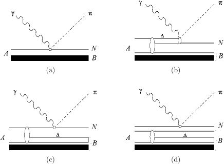
Figure 1: The diagrams illustrating the direct mechanisms of the $\pi N$ pair photoproduction on nuclei in the $A(\gamma,\pi N$)B reaction.

The first summand of the formula (4.5) corresponds to the interaction of the photon with $\Delta N$ system. We shall mark it $\rho^{S}_{\Delta\Delta}({X_{1};\tilde{X}_{1}})$. The second summand is $\rho^{C}_{\Delta\Delta}({X_{1};\tilde{X}_{1}})$, corresponds to the interaction of the photon with the nucleon core. As there is orthogonality of one-particle wave function, we shall get the expression for $\rho^{S}_{\Delta\Delta}(X_{1};\tilde{X}_{1})$ after the integration over the variable of the particles with numbers $3,...,A$

$$\rho^{S}_{\Delta\Delta}({X_{1};\tilde{X}_{1}})=\frac{{2}}{{A}}\sum\limits_{ij}{\int{dX_{2}}\Psi_{[{\beta_{i}\beta_{j}}]}^{\Delta N}({X_{1},X_{2}})\Psi_{[{\beta_{i}\beta_{j}}]}^{\Delta N\ast}({\tilde{X}_{1},X_{2}})}.$$

We will write the expression for the second summand in (4.5) $\rho^{C}_{\Delta\Delta}({X_{1};\tilde{X}_{1}})$ as

$$\rho^{C}_{\Delta\Delta}({X_{1};\tilde{X}_{1}})=\frac{{A-2}}{{A}}\sum\limits_{ij}{N_{\Delta\,ij}\int{d({X_{4},...,X_{A}})}\Psi_{({\beta_{i}\beta_{j}})^{-1}}^{N}({X_{1},X_{4},...,X_{A}})}\ \times$$

$$\times\ {\Psi_{({\beta_{i}\beta_{j}})^{-1}}^{N\ast}({\tilde{X}_{1},X_{4},...,X_{A}}}),$$

where $N_{\Delta\,ij}$ is the norm of wave function $\Psi_{[{\beta_{i}\beta_{j}}]}^{\Delta N}$, satisfying the relationship

$$\sum\limits_{ij}{N_{\Delta ij}=N_{\Delta}}.$$

Writing the wave function of the nucleon core $\Psi_{\left({\beta_{i}\beta_{j}}\right)^{-1}}^{N}$ in the form of decomposition

$$\Psi^{N}_{({\beta_{i}\beta_{j}})^{-1}}(X_{1},X_{4},...,X_{A})=A_{1;2...({A-1})\neq ij}^{S}\Psi_{\beta_{1}}(X_{1})\Psi^{N}_{({\beta_{i}\beta_{j}\beta_{1}})^{-1}}({X_{4},...,X_{A}})$$

and performing integration over the variables $X_{4},...,X_{A}$, we will get

$$\rho^{C}_{\Delta\Delta}({X_{1};\tilde{X}_{1}})=\frac{{1}}{{A}}\sum\limits_{ij,k\neq ij}{N_{\Delta ij}\Psi_{\beta_{k}}\left({X_{1}}\right)\Psi_{\beta_{k}}^{\ast}({\tilde{X}_{1}})}.$$

Using (3.5) and (4.2), we will write the summands of the expressions (4.5) as follows

$$\rho_{\Delta\Delta}=\rho^{\Delta}_{\Delta\Delta}+\rho^{N}_{\Delta\Delta}+\rho^{C}_{\Delta\Delta},$$

where

$$\rho^{\Delta}_{\Delta\Delta}({X_{1};\tilde{X}_{1}})=\phi_{\Delta}({m_{1}})\left[{{\,\frac{{1}}{{A}}\int{dx_{2}\,}\rho^{\Delta N}(x_{1},x_{2};\tilde{x}_{1},{x}_{2})}}\right]\phi_{\Delta}^{\ast}({\tilde{m}_{1}}),$$

$$\rho^{N}_{\Delta\Delta}({X_{1};\tilde{X}_{1}})=\phi_{N}({m_{1}})\left[{{\,\frac{{1}}{{A}}\int{dx_{2}\,}\rho^{\Delta N}(x_{2},x_{1};{x}_{2},\tilde{x}_{1})}}\right]\phi_{N}^{\ast}({\tilde{m}_{1}}),$$

$$\rho^{C}_{\Delta\Delta}({X_{1};\tilde{X}_{1}})=\phi_{N}(m_{1})\left[\,\frac{{1}}{{A}}\sum\limits_{ij}{N_{\Delta ij}\ \rho^{N}_{(\beta_{i}\beta_{j})^{-1}}(x_{1},\widetilde{x}{{}_{1}})}\right]\phi_{N}^{\ast}({\tilde{m}_{1}}),$$

$$\rho^{\Delta N}(x_{1},x_{2};\tilde{x}_{1},\tilde{x}_{2})=\sum\limits_{ij}\rho^{\Delta N}_{[ij]}(x_{1},x_{2};\tilde{x}_{1},\tilde{x}_{2}),$$

$$\rho^{\Delta N}_{[ij]}(x_{1},x_{2};\tilde{x}_{1},\tilde{x}_{2})={{\psi_{\left[{\beta_{i}\beta_{j}}\right]}^{\Delta N}({x_{1},x_{2}})\psi_{\left[{\beta_{i}\beta_{j}}\right]}^{\Delta N\ast}({\tilde{x}_{1},\tilde{x}_{2}})}},$$

$$\rho^{N}_{(\beta_{i}\beta_{j})^{-1}}(x_{1},\widetilde{x}{{}_{1}})=\sum_{k\neq ij}^{A}\psi_{\beta_{k}}(x_{1})\psi^{*}_{\beta_{k}}(\widetilde{x}{{}_{1}}).$$

In the expression for the density matrix $\rho^{\Delta}_{\Delta\Delta}({X_{1};\tilde{X}_{1}})$ the particle ”1” is an isobar. The reaction mechanism corresponding to the $\rho^{\Delta}_{\Delta\Delta}({X_{1};\tilde{X}_{1}})$, is illustrated by the diagram in Fig. 1b. In this case, the production of the pion results from the process $\gamma\Delta\to N\pi$, under which the virtual isobar taking up photon moves over to the real state and decays on the nucleon and the pion.

In expressions for the density matrix $\rho^{N}_{\Delta\Delta}({X_{1};\tilde{X}_{1}})$ and $\rho^{C}_{\Delta\Delta}({X_{1};\tilde{X}_{1}})$ the particle ”1” is nucleon. The reaction mechanisms corresponding to the $\rho^{N}_{\Delta\Delta}({X_{1};\tilde{X}_{1}})$ and $\rho^{C}_{\Delta\Delta}({X_{1};\tilde{X}_{1}})$ condition of the isobar configurations are illustrated by the diagrams in Fig. 1c and Fig. 1d. They differ by the composition and the condition of the baryons, forming the remaining nuclei.

5 Two-particle density matrix

Two-particle density matrix is used in the expressions for the square of the modulus of the exchange amplitude (2.2) for the reaction $A({\gamma,\pi N})B$. For calculation of the density matrix

$$\rho_{NN}({X_{1},X_{2};\tilde{X}_{1},\tilde{X}_{2}})=\int{d({X_{3},...,X_{A}})}\Psi_{N}({X_{1},X_{2},...,X_{A}})\Psi_{N}^{\ast}({\tilde{X}_{1},\tilde{X}_{2},...,X_{A}})$$ (5.1)

we will present the wave function $\Psi_{N}$ in the form of the expansion

$$\Psi_{N}(X_{1},X_{2},X_{3},...,X_{A})=\left(\frac{2N_{N}}{A(A-1)}\right)^{1/2}\sum_{ij}(-1)^{i+j+1}\Psi^{N}_{\beta_{i}\beta_{j}}(X_{1},X_{2})\ \times$$

$$\times\ \Psi^{N}_{(\beta_{i}\beta_{j})^{-1}}(X_{3},...,X_{A}),$$ (5.2)

where

$$\Psi_{\beta_{i}\beta_{j}}^{N}({X_{1},X_{2}})=A_{1;2}\Psi_{\beta_{i}}({X_{1}})\Psi_{\beta_{j}}(X_{2}).$$

After substituting (5.2) in (5.1), taking into account (4.2), we will get

$$\rho_{NN}({X_{1},X_{2};\tilde{X}_{1},\tilde{X}_{2}})=$$

$$\phi_{NN}\left({m_{1},m_{2}}\right)\left[{\frac{{2N_{N}}}{{A\left({A-1}\right)}}\sum\limits_{ij}{\psi_{\beta_{i}\beta_{j}}^{N}\left({x_{1},x_{2}}\right)}\psi_{\beta_{i}\beta_{j}}^{N\ast}\left({\tilde{x}_{1},\tilde{x}_{2}}\right)}\right]\phi_{NN}^{\ast}\left({\tilde{m}_{1},\tilde{m}_{2}}\right).$$

We shall go to the consideration of the density matrix $\rho_{\Delta\Delta}$

$$\rho_{\Delta\Delta}({X_{1},X_{2};\tilde{X}_{1},\tilde{X}_{2}})=\int{d({X_{3},...,X_{A}})}\Psi_{\Delta}({X_{1},X_{2},...,X_{A}})\Psi_{\Delta}^{\ast}{}({\tilde{X}_{1},\tilde{X}_{2},...,X_{A}}).$$

As a result of transformations of this expression, executed similarly in the previous section, the density matrix $\rho_{\Delta\Delta}$ may be written as

$$\rho_{\Delta\Delta}=\rho^{\Delta N}_{\Delta\Delta}+\rho^{N\Delta}_{\Delta\Delta}+\rho^{\Delta C}_{\Delta\Delta}+\rho^{NC}_{\Delta\Delta}+\rho^{CN}_{\Delta\Delta}+\rho^{C\Delta}_{\Delta\Delta}+\rho^{CC}_{\Delta\Delta},$$

where

$$\rho^{\Delta N}_{\Delta\Delta}({X_{1},X_{2};\tilde{X}_{1},\tilde{X}_{2}})=\phi_{\Delta N}({m_{1},m_{2}})\left[{\frac{{1}}{{A\left({A-1}\right)}}\ \rho^{\Delta N}(x_{1},x_{2};\tilde{x}_{1},\tilde{x}_{2})}\right]\phi_{\Delta N}^{\ast}({\tilde{m}_{1},\tilde{m}_{2}}),$$

$$\rho^{N\Delta}_{\Delta\Delta}({X_{1},X_{2};\tilde{X}_{1},\tilde{X}_{2}})=\phi_{\Delta N}({m_{2},m_{1}})\left[{\frac{{1}}{{A\left({A-1}\right)}}\ \rho^{\Delta N}(x_{2},x_{1};\tilde{x}_{2},\tilde{x}_{1})}\right]\phi_{\Delta N}^{\ast}\left({\tilde{m}_{2},\tilde{m}_{1}}\right),$$

$$\halign{\hbox to\displaywidth{$\hfil\displaystyle#\hfil$}\cr 0.0pt{\hfil$\displaystyle\rho^{\Delta C}_{\Delta\Delta}({X_{1},X_{2};\tilde{X}_{1},\tilde{X}_{2}})=\cr 0.0pt{\hfil$\displaystyle\phi_{\Delta N}({m_{1},m_{2}})\left[{\frac{{1}}{{A({A-1})}}\sum\limits_{ij}{\int{d({x_{3}})}}\rho^{\Delta N}_{[ij]}(x_{1},x_{3};\tilde{x}_{1},x_{3})\,\rho^{N}_{(ij)^{-1}}(x_{2};\tilde{x}_{2})}\right]\phi_{\Delta N}^{\ast}({\tilde{m}_{1},\tilde{m}_{2}}),\cr}}}$$

$$\halign{\hbox to\displaywidth{$\hfil\displaystyle#\hfil$}\cr 0.0pt{\hfil$\displaystyle\rho^{NC}_{\Delta\Delta}({X_{1},X_{2};\tilde{X}_{1},\tilde{X}_{2}})=\cr 0.0pt{\hfil$\displaystyle\phi_{NN}({m_{1},m_{2}})\left[{\frac{{1}}{{A({A-1})}}\sum\limits_{ij}{\int{d({x_{3}})}}\rho^{\Delta N}_{[ij]}(x_{3},x_{1};x_{3},\tilde{x}_{1})\,\rho^{N}_{(ij)^{-1}}(x_{2};\tilde{x}_{2})}\right]\phi_{NN}^{\ast}({\tilde{m}_{1},\tilde{m}_{2}}),\cr}}}$$

$$\halign{\hbox to\displaywidth{$\hfil\displaystyle#\hfil$}\cr 0.0pt{\hfil$\displaystyle\rho^{CN}_{\Delta\Delta}({X_{1},X_{2};\tilde{X}_{1},\tilde{X}_{2}})=\cr 0.0pt{\hfil$\displaystyle\phi_{NN}({m_{1},m_{2}})\left[{\frac{{1}}{{A({A-1})}}\sum\limits_{ij}{\int{d({x_{3}})}}\,\rho^{\Delta N}_{[ij]}(x_{3},x_{2};x_{3},\tilde{x}_{2})\,\rho^{N}_{(ij)^{-1}}(x_{1};\tilde{x}_{1})}\right]\phi_{NN}^{\ast}({\tilde{m}_{1},\tilde{m}_{2}}),\cr}}}$$

$$\halign{\hbox to\displaywidth{$\hfil\displaystyle#\hfil$}\cr 0.0pt{\hfil$\displaystyle\rho^{C\Delta}_{\Delta\Delta}({X_{1},X_{2};\tilde{X}_{1},\tilde{X}_{2}})=\cr 0.0pt{\hfil$\displaystyle\phi_{\Delta N}({m_{2},m_{1}})\left[{\frac{{1}}{{A({A-1})}}\sum\limits_{ij}{\int{d({x_{3}})}}\,\rho^{\Delta N}_{[ij]}(x_{2},x_{3};\tilde{x}_{2},{x}_{3})\,\rho^{N}_{(ij)^{-1}}(x_{1};\tilde{x}_{1})}\right]\phi_{\Delta N}^{\ast}({\tilde{m}_{2},\tilde{m}_{1}}),\cr}}}$$

$$\rho^{CC}_{\Delta\Delta}({X_{1},X_{2};\tilde{X}_{1},\tilde{X}_{2}})=$$

$$\phi_{NN}({m_{1},m_{2}})\left[{\frac{{2}}{{A\left({A-1}\right)}}\sum\limits_{ij}{N_{\Delta ij}\ \rho^{NN}_{(ij)^{-1}}(x_{1},x_{2};\tilde{x}_{1},\tilde{x}_{2})}}\right]\phi_{NN}^{\ast}({\tilde{m}_{1},\tilde{m}_{2}}),$$

$$\rho^{NN}_{(ij)^{-1}}(x_{1},x_{2};\tilde{x}_{1},\tilde{x}_{2})=\sum\limits_{kl\neq ij}{\psi_{\beta_{k}\beta_{l}}^{N}({x_{1},x_{2}})}\psi_{\beta_{k}\beta_{l}}^{N\ast}({\tilde{x}_{1},\tilde{x}_{2}}).$$

The exchange amplitudes, corresponding to the matrix $\rho^{N\Delta}_{\Delta\Delta}$ and $\rho^{C\Delta}_{\Delta\Delta}$ are zero, because of the orthogonality of the wave functions $\phi_{N}\left({m_{2}}\right)$ and $\phi_{\Delta}\left({m_{2}}\right)$. The remaining six summands $\rho_{NN},$ $\rho^{\Delta N}_{\Delta\Delta},$ $\rho^{\Delta C}_{\Delta\Delta},$ $\rho^{NC}_{\Delta\Delta},$ $\rho^{CN}_{\Delta\Delta}$ and $\rho^{CC}_{\Delta\Delta}$ of the two-particle density matrix correspond to the mechanism of the reactions in the usual space, which are illustrated by the diagram shown in Fig. 2 in the same order.

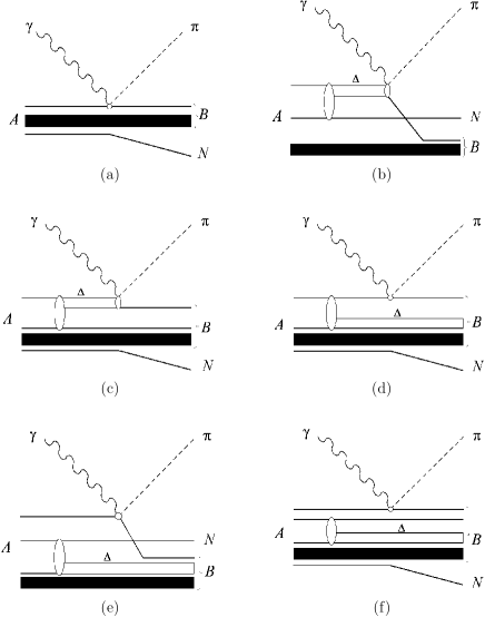
Figure 2: The diagrams illustrating the exchange mechanisms of the $\pi N$ pair photoproduction on nuclei in the $A(\gamma,\pi N$)B reaction.

6 Transition operator

With the help of the formula

$$<x^{\prime}|t_{\gamma B\pi}|x>=\sum_{m^{\prime}m}\phi^{*}_{N}(m^{\prime})<X^{\prime}|t_{\gamma\pi}|X>\phi_{B}(m),$$

matrix element of the operator $t_{\gamma\pi}$ between the one-particle intrinsic states defines the transition operator $<x^{\prime}|t_{\gamma B\pi}|x>$ in the configuration space, which acts on the space $\mathbf{r}$, spin s, and isospin t coordinates.

Using the S-matrix approach for the description of an elementary process $\gamma B\rightarrow N\pi$, we will find the transition operator $t_{\gamma B\pi}$. We will suppose that S-matrix has the standard expansion in power of the interaction Lagrangian, in which the strong interaction fields of the nucleon, pion and isobar, the vector potential of photon are the operators acting on the space $\mathbf{r}$, spin s, and isospin t coordinates. We will write the Lagrangian of the strong interaction baryon fields and the pion field as $L_{s}=\textbf{j}_{\pi}(\textbf{r},t)\boldsymbol{\phi}(\textbf{r},t)$, where $\textbf{j}_{\pi}(\textbf{r},t)$ is the pion current. The Lagrangian of the electromagnetic interaction may be written as $L_{\gamma}=j_{\mu}(\textbf{r},t)A^{\mu}(\textbf{r},t)$, where $j_{\mu}(\textbf{r},t)$ is the electromagnetic current. Then, the transition operator $t_{\gamma B\pi}$ may be written as

$$t_{\gamma B\pi}=\boldsymbol{\varphi}_{a}^{+}\textbf{t}_{\gamma B\pi}^{\mu}\ {\epsilon}^{\lambda}_{\mu}.$$

Here ${\epsilon}^{\lambda}$ is 4-vector of the photon polarization; $\boldsymbol{\varphi_{a}}$ is the covariant unit vector of the cyclical basis describing the isotopic state of the pion; index a takes on the values +, 0, -, which fit with the positive, neutral and negative pions;

$$\textbf{t}_{\gamma B\pi}^{\mu}=\int d\textbf{r}d\textbf{r}^{\prime}e^{i(\textbf{p}_{\gamma}\,\textbf{r}-\textbf{p}_{\pi}\,\textbf{r}^{\prime})}\int dte^{-iE_{\gamma}t}T(j_{\mu}(\textbf{r},t)\textbf{j}_{\pi}(\textbf{r}^{\prime},0))|_{B\rightarrow N},$$ (6.1)

where index $B\rightarrow N$ under T-product of the currents designates that it necessarily leaves those components of the electromagnetic and pion currents, which give rise to the $N\rightarrow N$ and the $\Delta\rightarrow N$ transitions. The expression of the current comes from the interaction Lagrangian constructing from the photon, nucleon, $\Delta$-isobar and pion fields. Using the operator (6.1), we will go to the momentum representation of the matrix element $<x^{\prime}|\textbf{t}_{\gamma B\pi}^{\mu}|x>$ and insert the complete set of the intermediate single-particle baryon and meson states with the minimal masses of the baryons and the pions. As a result, we will obtain

$$<x^{\prime}|\textbf{t}_{\gamma B\pi}^{\mu}|x>=\int d\textbf{p}_{B}e^{i\textbf{p}_{N}\textbf{r}^{\prime}}\sum_{m_{\sigma_{N}},m_{\tau_{N}},m_{\sigma_{B}},m_{\tau_{B}}}\xi^{*}_{m_{\sigma_{N}},m_{\tau_{N}}}(s^{\prime},t^{\prime})\,\times$$

$$\times\,<m_{\sigma_{N}},m_{\tau_{N}}|\textbf{T}^{\mu}_{\gamma B\rightarrow N\pi}(\textbf{p}_{N},\textbf{p}_{B})|m_{\sigma_{B}},m_{\tau_{B}}>\xi_{m_{\sigma_{B}},m_{\tau_{B}}}(s,t)e^{-i\textbf{p}_{B}\textbf{r}}.$$ (6.2)

Here B and N are the indices of the initial baryon and the final nucleon; $\textbf{p}_{B}$ and $\textbf{p}_{N}$ are the momenta of the baryon and the nucleon for the process $\gamma B\rightarrow\pi N$, $\textbf{p}_{N}=\textbf{p}_{B}+\textbf{q}$, where $\textbf{q}=\textbf{p}_{\gamma}-\textbf{p}_{\pi}$ is the transfer momentum,  $\xi_{m_{\sigma_{N}},m_{\tau_{N}}}$ and  $\xi_{m_{\sigma_{B}},m_{\tau_{B}}}$ are the spin-isospin wave functions of the nucleon and the baryon. If it designates: $\alpha\equiv\textbf{p},m_{\sigma},m_{\tau}$ is the baryon state index; n is the index of the intermediate baryon, $\alpha_{\pi^{a}}$ is the index of the pion, then

$$<m_{\sigma_{N}},m_{\tau_{N}}|\textbf{T}^{\mu}_{\gamma B\rightarrow N\pi}(\textbf{p}_{N},\textbf{p}_{B})|m_{\sigma_{B}},m_{\tau_{B}}>\ =$$

$$\frac{(2\pi)^{3}}{i}\left[\sum_{n=N,\Delta}\frac{<\alpha_{N}|j^{\mu}(0,0)|\alpha_{n}><\alpha_{n}|\textbf{j}_{\pi}(0,0)|\alpha_{B}>}{E_{\gamma}+E_{n}-E_{N}-i\varepsilon}\right.+$$

$$+\sum_{\widetilde{n}=N,\Delta}\frac{<\alpha_{N}|\textbf{j}_{\pi}(0,0)|\alpha_{\widetilde{n}}><\alpha_{\widetilde{n}}|j^{\mu}(0,0)|\alpha_{B}>}{E_{\widetilde{n}}-E_{\gamma}-E_{B}-i\varepsilon}-$$

$$-\left.2\frac{E^{2}_{\widetilde{\pi}}}{E_{\pi}}\sum_{b}\frac{<\alpha_{\pi^{a}}|j^{\mu}(0,0)|\alpha_{\widetilde{\pi}^{b}}><\alpha_{N}|\textbf{j}_{\pi}(0,0)|\alpha_{B}>}{E^{2}_{\widetilde{\pi}}-\textbf{p}^{2}_{\widetilde{\pi}}-m^{2}_{\pi}}+i<\alpha_{N}|\textbf{j}^{\mu}_{\gamma\pi NB}|\alpha_{B}>\ \right],$$

where $\textbf{p}_{n}=\textbf{p}_{B}-\textbf{p}_{\pi}$, $\textbf{p}_{\widetilde{n}}=\textbf{p}_{\gamma}+\textbf{p}_{B}$ and $\textbf{p}_{\widetilde{\pi}}=-\textbf{q}$ are the momenta of the intermediate baryons and mesons, $E_{n}=(\textbf{p}^{2}_{n}+m^{2}_{n})^{1/2}$, $E_{\widetilde{n}}=(\textbf{p}^{2}_{\widetilde{n}}+m^{2}_{\widetilde{n}})^{1/2}$, $E_{\widetilde{\pi}}=E_{\gamma}-E_{\pi}$.

The matrix elements of the currents are written by means of the nonrelativistic currents as

$$<\alpha_{2}|j^{\mu}(0,0)|\alpha_{1}>\,=\frac{1}{2}(E_{2}E_{1})^{-1/2}\,\xi^{*}_{m_{\sigma_{2}},m_{\tau_{2}}}j^{\mu,B_{2}\leftarrow B_{1}}(\textbf{p}_{2},\textbf{p}_{1})\,\xi_{m_{\sigma_{1}},m_{\tau_{1}}},$$

$$<\alpha_{2}|\textbf{j}_{\pi}(0,0)|\alpha_{1}>\,=\frac{1}{2}(E_{2}E_{1})^{-1/2}\,\xi^{*}_{m_{\sigma_{2}},m_{\tau_{2}}}\textbf{j}_{\pi}^{B_{2}\leftarrow B_{1}}(\textbf{p}_{2},\textbf{p}_{1})\,\xi_{m_{\sigma_{1}},m_{\tau_{1}}},$$

$$<\alpha_{\pi^{a}}|j^{\mu}(0,0)|\alpha_{\widetilde{\pi}^{b}}>\,=\frac{1}{2}\,(E_{\pi}E_{\widetilde{\pi}})^{-1/2}\boldsymbol{\varphi}^{+}_{a}\,j^{\mu,\pi\leftarrow\pi}(\textbf{p}_{\pi},\textbf{p}_{\widetilde{\pi}})\,\boldsymbol{\varphi}_{b}.$$

The explicit expressions of nonrelativistic currents are

$$\textbf{j}_{\gamma}^{N\leftarrow N}\left({\textbf{p}_{2},\textbf{p}_{1}}\right)=\frac{{e}}{{2m_{N}}}\left[{\left({\textbf{p}_{2}+\textbf{p}_{1}}\right)\frac{{1+\tau_{3}}}{{2}}-i\left({\textbf{p}_{2}-\textbf{p}_{1}}\right)\times\boldsymbol{\sigma}\left({\frac{1+\tau_{3}}{2}\mu_{p}+\frac{1-\tau_{3}}{2}\mu_{n}}\right)}\right],$$

$$\textbf{j}_{\gamma}^{N\leftarrow\Delta}\left({\textbf{p}_{2},\textbf{p}_{1}}\right)=i\frac{{e}}{{2m_{N}}}\mu_{\gamma N\Delta}\left[{\left({\textbf{p}_{2}-\textbf{p}_{1}}\right)\times\textbf{S}^{+}}\right]T^{+}_{3},$$

$$\textbf{j}_{\gamma}^{\Delta\leftarrow\Delta}\left({\textbf{p}_{2},\textbf{p}_{1}}\right)=\frac{{e}}{{2m_{\Delta}}}{\left({\textbf{p}_{2}+\textbf{p}_{1}}\right)\frac{{1+\Theta_{3}}}{{2}}-i\,\frac{e}{2m_{N}}\,\mu_{\Delta^{++}}\left[\left({\textbf{p}_{2}-\textbf{ p}_{1}}\right)\times\boldsymbol{\Sigma}_{\Delta}\right]\frac{{1+\Theta_{3}}}{{4}}},$$

$$\textbf{j}_{\gamma}^{\pi N\leftarrow\Delta}=ie\,\frac{{f_{\pi N\Delta}}}{{m_{\pi}}}\,\textbf{S}^{+}\,\textbf{T}^{+},\ \ \ \textbf{j}_{\gamma}^{\pi N\leftarrow N}=ie\,\frac{{f_{\pi NN}}}{{m_{\pi}}}\,\boldsymbol{\sigma}\boldsymbol{\tau},$$

$$\textbf{j}_{\gamma}^{\pi\leftarrow\pi}\left({\textbf{p}_{2},\textbf{p}_{1}}\right)=\frac{e}{2}\left({\textbf{p}_{2}-\textbf{p}_{1}}\right),\ \ \textbf{j}_{\pi}^{\Delta\leftarrow\Delta}\left({\textbf{p}_{2},\textbf{p}_{1}}\right)=-i\,\frac{{f_{\pi\Delta\Delta}}}{{m_{\pi}}}\,\left({\textbf{p}_{2}-\textbf{p}_{1}}\right)\cdot\boldsymbol{\Sigma}_{\Delta}\textbf{T}_{\Delta},$$

$$\textbf{j}_{\pi}^{N\leftarrow N}\left({\textbf{p}_{2},\textbf{p}_{1}}\right)=-i\,\frac{{f_{\pi NN}}}{{m_{\pi}}}\,\ \left({\textbf{p}_{2}-\textbf{p}_{1}}\right)\cdot\boldsymbol{\sigma}\boldsymbol{\tau},$$

$$\textbf{j}_{\pi}^{N\leftarrow\Delta}\left({\textbf{p}_{2},\textbf{p}_{1}}\right)=-i\,\frac{{f_{\pi N\Delta}}}{{m_{\pi}}}\,\ \left({\textbf{p}_{2}-\textbf{p}_{1}}\right)\cdot\textbf{S}^{+}\mathop{\textbf{T}^{+}}\limits.$$

Here S is transition spin operator which converts the spin-1/2 state into the spin-3/2 state. The matrix S is defined as

$$\textbf{S}_{m_{\frac{3}{2}},\,m_{\frac{1}{2}}}=\sum_{m}C_{\frac{1}{2},\,m_{\frac{1}{2}};\,1,\,m}^{\frac{3}{2},\,m_{\frac{3}{2}}}\textbf{e}_{m},$$

where the Condon and Shortly phase convention for Clebsch-Gordon coefficients has been used and $\textbf{e}_{m}$ is unit vector in the spherical basis. The matrix T is transition isospin operator which converts the isospin-1/2 state into the isospin-3/2 state. The matrices $\boldsymbol{\Sigma}_{\Delta}$ and $\textbf{T}_{\Delta}$ are defined as

$$\boldsymbol{\Sigma}_{\Delta}=\sum_{l=1}^{3}S_{l}\boldsymbol{\sigma}S_{l}^{+},\ \ \ \ \textbf{T}_{\Delta}=\sum_{l=1}^{3}T_{l}\boldsymbol{\tau}T_{l}^{+}.$$

We shall notice that the matrices $\boldsymbol{\Sigma}_{\Delta}$ and $\textbf{T}_{\Delta}$ are

$$\boldsymbol{\Sigma}_{\Delta}=\frac{\boldsymbol{\Sigma}}{3}\hskip 5.69054pt\mbox{and}\hskip 5.69054pt\textbf{T}_{\Delta}=\frac{\boldsymbol{\Theta}}{3},$$

where $\boldsymbol{\Sigma}(\boldsymbol{\Theta})$ is the Pauli operator for the $\Delta$ spin(isospin). The proton and neutron magnetic moments of the nucleon are accordingly $\mu_{p}=2.79$ and $\mu_{n}=-1.91$ in terms of nuclear magnetons. The magnetic moment of the isobar is taken to be $\mu_{\Delta^{++}}$= 4.52 in terms of nuclear magnetons, using the value obtained from a soft-photon analysis of pion-proton bremsstrahlung data near the $\Delta^{++}$ resonance [20]. Using the excitation strengths $G_{M}$=0.28, as obtained from the analysis of $\gamma N$ data in the $\Delta$-resonance region [21], we calculated the value of the transition magnetic moment $\mu_{\gamma N\Delta}$=3.42 in terms of nuclear magnetons. The $\pi NN$ coupling constants is $f_{\pi NN}^{\,2}/4\pi=0.08$. For the $\pi N\Delta$ coupling constant we take the value $f_{\pi N\Delta}$ = 2.123 obtained from the decay $\Delta\rightarrow\pi N$ [22]. The $\pi\Delta\Delta$ coupling constants is $f_{\pi\Delta\Delta}$ = $4/5f_{\pi NN}$, as predicted by the trivial quark model.

The result (6.2) for $<x^{\prime}|\textbf{t}_{\gamma B\pi}^{\mu}|x>$ answers, in general, to the non-locale interaction that brings about the need of the calculation of multivariate integral on $\textbf{p}_{B},$ $\textbf{r}^{\prime},$ r. Supposing the momentum $\textbf{p}_{N}$ in the operator $\textbf{T}_{\gamma B\to N\pi}^{\mu}({\textbf{p}_{N},\textbf{p}_{B}})$ is fixed $\textbf{p}_{N}=\widetilde{\textbf{p}}$ gives the local transition operator $<x^{\prime}|t_{\gamma{\rm B}\pi}^{\mu}|x>$

$$<x^{\prime}|t_{\gamma{\rm B}\pi}^{\mu}|x>=\delta({\textbf{r}^{\prime}-\textbf{r}})e^{i\,({\textbf{p}_{\gamma}\textbf{r}-\textbf{p}_{\pi}\textbf{r}^{\prime}})}<s^{\prime},t^{\prime}|T_{\gamma{\rm B}\pi}^{\mu}({\tilde{\textbf{p}},\tilde{\textbf{p}}-\textbf{q}})|s,t>.$$

Here

$$<s^{\prime},t^{\prime}|\textbf{T}_{\gamma{\rm B}\pi}^{\mu}({\tilde{\textbf{p}},\tilde{\textbf{p}}-\textbf{q}})|s,t>\,=\,\sum_{m_{\sigma_{N}},m_{\tau_{N}},m_{\sigma_{B}},m_{\tau_{B}}}{\zeta_{m_{\sigma_{N}},m_{\tau_{N}}}^{\ast}({s^{\prime},t^{\prime}})}\,\times$$

$$\times\ <m_{\sigma_{N}},m_{\tau_{N}}|\textbf{T}^{\mu}_{\gamma B\rightarrow N\pi}({\tilde{\textbf{p}},\tilde{\textbf{p}}-\textbf{q}})|m_{\sigma_{B}},m_{\tau_{B}}>\zeta_{m_{\sigma_{B}},m_{\tau_{B}}}({s,t}).$$

Calculating the amplitude of the transition $\gamma B\to N\pi$, as momentum $\widetilde{\textbf{p}}$, we shall take the momentum, which is canonically conjugate to the coordinate r in the nucleon wave function. For the amplitude, corresponding to the diagram on fig. 1a, the momentum $\tilde{\textbf{p}}$ is the momentum $\textbf{p}_{n}$ of the free nucleon. In the exchange amplitude the momentum $\tilde{\textbf{p}}$ is the integration variable.

Using the explicit form of the expression of non-relativistic currets, the transition operator $t_{\gamma\Delta\pi}$ may be written as

$$t_{\gamma\Delta\pi}=\boldsymbol{\varphi}_{a}^{+}\,\sum^{4}_{i=1}\sum^{3}_{j=1}f_{ij}\,M_{i}\,\textbf{I}_{j},$$

where $M_{i}$ are the independent spin structures

$$\begin{array}[]{ll}M_{1}=\boldsymbol{\varepsilon}^{\lambda}\cdot\mathbf{S}^{+};&M_{2}=i\boldsymbol{\sigma}\cdot[\mathbf{p}_{\gamma}\times\boldsymbol{\varepsilon}^{\lambda}]\,\mathbf{p}_{\pi}\cdot\mathbf{S}^{+};\\ &\\ M_{3}=\mathbf{p}_{\pi}\cdot\boldsymbol{\varepsilon}^{\lambda}\,\mathbf{p}_{\gamma}\cdot\mathbf{S}^{+};&M_{4}=\mathbf{p}_{\pi}\cdot\boldsymbol{\varepsilon}^{\lambda}\,\mathbf{p}_{\pi}\cdot\mathbf{S}^{+}.\end{array}$$

Here $\boldsymbol{\varepsilon}^{\lambda}$ is 3 -vector of the photon polarization.

The isospin structures are

$$\mathbf{I}_{1}=\mathbf{T}^{+},\ \mathbf{I}_{2}=\boldsymbol{\tau}T^{+}_{3},\ \mathbf{I}_{3}=\tau_{3}\mathbf{T}^{+}$$

The values $f_{ij}$ are

$$\begin{array}[]{ll}\displaystyle f_{11}=\alpha\,\left[-\frac{\mu_{\Delta^{++}}}{6\,a}\,\mathbf{p}_{\pi}\mathbf{p}_{\gamma}+2\,m_{N}\right],&\displaystyle f_{12}=\alpha\left[\frac{\mu_{\Delta^{++}}}{3\,a}-\frac{F}{3\,b}\right]\mathbf{p}_{\pi}\mathbf{p}_{\gamma},\\ \displaystyle f_{13}=\alpha\left[-\frac{\mu_{\Delta^{++}}}{2\,a}+\frac{2F}{9\,b}\right]\mathbf{p}_{\pi}\mathbf{p}_{\gamma},&\displaystyle f_{21}=\alpha\left[-\frac{\mu_{\Delta^{++}}}{12\,a}+\frac{\mu_{p}+\mu_{n}}{2\,c}\right],\\ \displaystyle f_{22}=\alpha\left[\frac{\mu_{\Delta^{++}}}{6\,a}-\frac{F}{b}\right],&\displaystyle f_{23}=\alpha\left[-\frac{\mu_{\Delta^{++}}}{4\,a}+\frac{2\,F}{3\,b}+\frac{\mu_{p}-\mu_{n}}{2\,c}\right],\\ \displaystyle f_{31}=\alpha\left[\frac{\mu_{\Delta^{++}}}{6\,a}-\frac{2\,m_{N}}{d}\right],&\displaystyle f_{32}=\alpha\left[-\frac{\mu_{\Delta^{++}}}{3\,a}+\frac{F}{3\,b}\right],\\ \displaystyle f_{33}=\alpha\left[\frac{\mu_{\Delta^{++}}}{2\,a}-\frac{2\,F}{9\,b}\right],&\displaystyle f_{41}=\alpha\frac{2\,m_{N}}{d},\\ \displaystyle f_{42}=0,&\displaystyle f_{43}=0.\end{array}$$

Here

$$\begin{array}[]{ll}\displaystyle F=\mu_{\gamma N\Delta}\,\frac{{f_{\pi\Delta\Delta}}}{f_{\pi N\Delta}},&\displaystyle\alpha=i\,\frac{e}{2m_{N}}\ \frac{f_{\pi N\Delta}}{m_{\pi}},\\ &\\ a=E_{\Delta}+E_{\gamma}-E_{a}+\frac{i}{2}\Gamma_{\Delta},&b=E_{\Delta}-E_{\pi}-E_{b}+i\varepsilon,\\ &\\ c=E_{\Delta}-E_{\pi}-E_{c}+i\varepsilon,&d=(\mathbf{p}_{N}-\mathbf{p}_{\Delta})^{2}-(E_{N}-E_{\Delta})^{2}+m^{2}_{\pi}+i\varepsilon,\end{array}$$

$$E_{a}=((\mathbf{p}_{\Delta}+\mathbf{p}_{\gamma})^{2}+m_{\Delta}^{2})^{1/2},\,E_{b}=((\mathbf{p}_{\Delta}-\mathbf{p}_{\pi})^{2}+m_{\Delta}^{2})^{1/2},\,E_{c}=((\mathbf{p}_{\Delta}-\mathbf{p}_{\pi})^{2}+m_{N}^{2})^{1/2}.$$

We shall use the non-relativistic operator of Blomqvist-Laget [23] as the transition operator $t_{\gamma N\pi}$ .

7 Cross section of the $A({\gamma,\pi N})B$ reaction

Following from the consideration of one- and two-particle density matrixes, an account of the isobar configurations in the atomic nuclei results in a significant increase of possible direct and exchange mechanisms of the reactions in the usual space. One-particle and two-particle density matrixes present themselves as some combinations of one-particle wave functions of the nucleons bound in nuclei $\psi_{\beta_{i}}({x})$ and wave function $\psi_{[{\beta_{i}\beta_{j}}]}^{\Delta N}({x_{1},x_{2}})$, describing the $\Delta N$ system. Separate components of one-particle and two-particle density matrixes are connected with different mechanisms of considered reaction. For qualitative estimation of the kinematic area, where different mechanisms of the reactions are shown, the momentum distributions of the isobar $\rho^{\Delta}$ and proton $\rho^{N}$ of nucleus ¹²C defined as

$$\rho^{N}({p})=\sum\limits_{i}{\int{dy_{{}_{N}}}\,\Phi_{\beta_{i}}^{\ast}({y_{{}_{N}}})}\,\delta({p-p_{{}_{N}}})\delta_{{}_{1/2},m_{\tau_{i}}}\Phi_{\beta_{i}}({y_{{}_{N}}})/\,p^{2},$$

$$\rho^{\Delta}({p})=\sum\limits_{ij}{\int{d(y_{{}_{\Lambda}},y_{{}_{N}})\,}\Phi_{[{\beta_{i}\beta_{j}}]}^{\Delta N\ast}\,({y_{{}_{\Delta}},y_{{}_{N}}})}\delta({p-p_{{}_{\Delta}}})\Phi_{[{\beta_{i}\beta_{j}}]}^{\Delta N}({y_{{}_{\Delta}},y_{{}_{N}}})/\,p^{2}$$

are given in Fig. 3, where $y\equiv\mathbf{p},s,t$; $\Phi_{\beta_{i}}({y}_{{}_{N}})$ and $\Phi_{[{\beta_{i}\beta_{j}}]}^{\Delta N}({y_{{}_{\Lambda}},y_{{}_{{}_{N}}}})$ are the Fourier transforms of the wave functions $\psi_{\beta_{i}}({x}_{{}_{N}})$ and $\psi_{[{\beta_{i}\beta_{j}}]}^{\Delta N}\left({x_{{}_{\Lambda}},x_{{}_{{}_{N}}}}\right).$

Figure 3: The momentum distributions of the $\Delta$-isobar (solid curve) and protons (dashed curve) of nucleus ¹²C

Let us consider the direct mechanisms of the reaction. First of all it is necessary to note that all four mechanisms of the reaction shown in Fig. 1(a–d), give contributions to the cross section of the photoproduction of the $\pi^{+}n,$ $\pi^{-}p,$ $\pi^{0}p$ and $\pi^{0}n$ pairs. The contributions to the cross section of the photoproduction of the $\pi^{+}p$ and $\pi^{-}n$ pairs are due to the mechanism in Fig. 1b. So, these two reactions are perspective for the study of the virtual states of the isobar in a nucleus. Since the density of the momentum distribution of the nucleon under small momentum is by several orders more than the density of the momentum distribution of the ${\Delta}$-isobar, the mechanisms of the reactions corresponding to the diagrams in Fig. 1a and Fig. 1d practically completely define the behavior of the cross section of reactions in this kinematic area. At large momentum transfer to the nucleus exceeding 400 MeV/c, the mechanisms of the reactions corresponding to the diagrams in Fig. 1b and in Fig. 1c dominate. The relative contribution of these diagrams is defined, basically, by the probability of the $\gamma N\rightarrow N\pi$ and $\gamma\Delta\to N\pi$ transitions. The direct mechanism of a pion photoproduction corresponding to the diagrams in Fig. 1a and taking into account only the nucleon configurations is analysed in detail in Refs. [24, 25, 26].

The exchange mechanisms of the reactions shown in Fig. 2(a–f) may be divided into two groups. One group includes the mechanisms in which the nucleon belonging to the nucleon core of the nucleus becomes free. Manifestations of the exchange mechanism of the neutral pion photoproduction within the framework of the model, taking into account only the nucleon configurations of the nuclei, were analysed in the works [27, 28]. The contribution of the appropriate exchange transition amplitudes quickly decreases with growing of the nucleon energy and concentrates near the kinematic area of the coherent pion photoproduction on the residual nucleus, in range of small momentum transfer $\textbf{p}_{\gamma}-\textbf{p}_{\pi}$. Another group contains mechanisms of the reactions in which the nucleon of the $\Delta N$ system becomes free. These mechanisms of the $\pi^{+}p$ pair photoproduction were considered in the work [29]. The contribution of them to the cross section of the reactions concentrated in the considerably greater range of the nucleon momentum, practically coinciding with range of definition of the virtual isobar momentum distribution.

The cross section corresponding to the different pion-nucleon pair production mechanisms is numerically estimated in respect of ¹²C$({\gamma,\pi^{-}p})^{11}$C and ¹²C$({\gamma,\pi^{+}p})^{11}$Be reactions. The differential cross sections are calculated for that mechanisms in which the proton momentum in the final states can be large enough for the experimental checking of the model predictions by means of simultaneous registration of the pion and the proton in the experiment. These are, first of all, the direct mechanisms of the reactions and the exchange mechanisms in which the nucleon of the $\Delta N$ systems becomes free.

The cross section of the reaction ¹²C$({\gamma,\pi^{-}p})^{11}$C is calculated in the kinematic area in which the experimental data [10] were interpreted [11] as the manifestation of a quasibound isobar-nucleus states.

The experiment [10] was performed in the $\Delta(1232)$ resonance energy region using the bremsstrahlung photon beam from the Tomsk synchrotron. The pions and protons were detected in coincidence by two spectrometers placed on opposite sides of the photon beam. Figure 4 shows the dependence of the differential reaction yield $d^{4}Y/dE_{p}d\Omega_{p}dE_{\pi}d\Omega_{\pi}$ as the function of the opening angle $\theta_{\pi p}=\theta_{\pi}+\theta_{p}$, where $\theta_{\pi}$ and $\theta_{p}$ are the pion and proton polar angles, connected with differential cross section

$$\frac{{d^{3}\sigma}}{{dE_{p}d\Omega_{p}d\Omega_{\pi}}}=\left({2\pi}\right)^{-5}\frac{{p_{\pi}^{3}p_{p}E_{p}E_{R}}}{{4E_{\gamma}\left|{E_{R}p_{\pi}^{2}-E_{\pi}p_{\pi}p_{R}}\right|}}\overline{\left|{{\rm{T}}_{fi}}\right|^{2}}$$

by the relation

$$\frac{d^{4}Y}{dE_{p}d\Omega_{p}dE_{\pi}d\Omega_{\pi}}=\frac{{d^{3}\sigma}}{{dE_{p}d\Omega_{p}d\Omega_{\pi}}}f(E_{\gamma})\left|\frac{\partial E_{\gamma}}{\partial E_{\pi}}\right|.$$

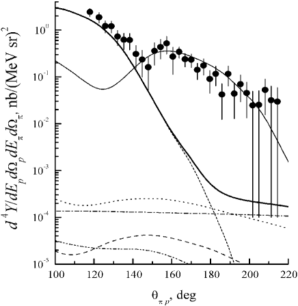
Figure 4: Differential yield of the ¹²C$({\gamma,\pi^{-}p})$ reaction for $E_{\mbox{max}}=500$ MeV versus the opening angle $\theta_{\pi p}$. Thin solid curve: the $\Delta$-nucleus model [11], in which the existence of the ¹¹B_Δ quasibound isobar-nucleus states is assumed in the intermediate state of the ¹²C$({\gamma,\pi^{-}p})p\,^{10}$B reaction, short dashed line: quasifree pion photoproduction, dashed and doted curves: direct mechanisms of the ¹²C$({\gamma,\pi^{-}p})^{11}$C reaction, corresponding to diagrams in Fig. 1b and Fig. 1c, dasheddotted curves with one and two points: the exchange mechanisms of the reaction, corresponding to the diagrams in Fig. 2e and Fig. 2b, thick solid curve: the total contribution to the cross section of the nucleon and isobar configurations, data are taken from Ref. [10].

Here $f({E_{\gamma}})$ is the bremsstrahlung spectrum, normalized as

$$\int{dE_{\gamma}f\left({E_{\gamma}}\right)}E_{\gamma}=E_{\mbox{max}},$$

where $E_{\mbox{max}}$ is the maximal energy of the bremsstrahlung, $\overline{\left|{{\rm{T}}_{fi}}\right|^{2}}$ is the square of the modulus of the reaction amplitude ${\rm{T}}_{fi}$, averaged over photon polarization states and summed over proton and residual nucleus states and which is connected with the matrix element of the $T_{fi}$ in (2.1) by the relation

$$T_{fi}=\left({2\pi}\right)^{3}\delta\left({\textbf{p}_{\gamma}-\textbf{p}_{\pi}-\textbf{p}_{p}-\textbf{p}_{R}}\right){\rm{T}}_{fi}.$$

In Fig. 4 both the experimental data and the calculated reaction yields are averaged over the proton energy in the interval of $60-140$ MeV and over the pion energy in the interval of $102-148$ MeV.

Kinematically, in Fig. 4 the small opening angle region corresponds to smaller momentum transfers to the residual nuclear system. In this kinematical region the differential yield of the quasifree photoproducton of the pions is dominant as it is indicated by short dashed line in Fig. 4. The differential yield includes the contributions from two mechanisms of the reaction corresponding to the diagrams in Fig. 1a and Fig. 1d. The pion production in this case occurs at interaction of the photon with the nucleon in the state which is lower than the Fermi level. The wave function of the nucleon bound state is calculated using the harmonic-oscillator shell model which reproduces the charge radius of the ¹²C nucleus. Final-state interaction is taken into account through optical model. As can be seen, the agreement between the data [10] and the quasifree pion photoproduction model both for shape and magnitude is reasonable for opening angles up to $145^{\circ}$.

In this paper we are primarily interested in the large opening angle region, where the momentum transfer is relatively large and where discrepancy is observed between data [10] and the quasifree pion photoproduction model.

In Fig. 4 the thin solid curve indicates the angular dependence of the differential reaction yield calculated within the framework of the $\Delta$-nucleus model [11], in which the existence of the ¹¹B_Δ quasibound isobar-nucleus states is assumed in the intermediate state of the ¹²C$({\gamma,\pi^{-}p})p\,^{10}$B reaction. The $\Delta$-nucleus model [11] predicts the functional dependence of the cross section but not its absolute value; therefore, the reaction yield represented by the thin solid curve was normalized by fitting to the data points in the opening angle range $\theta_{\pi p}=145^{\circ}-215^{\circ}$.

The dashed and dotted curves present the contributions to the cross section of the two direct mechanisms of the reactions, corresponding to diagrams in Fig. 1b and Fig. 1c, in which the product of the pions results from the interaction of the photon with the $\Delta N$ system. The shapes of two these curves follow substantially the momentum distribution of the isobar and the nucleon of the $\Delta N$ system.

The contributions of the exchange mechanisms of the reaction to the cross section, corresponding to the diagrams in Fig. 2e and Fig. 2b are presented by the dashed-dotted curves with one and two points. In the isobar exchange amplitude (Fig. 2b) the large opening angle region corresponds to higher momentum transfers q in the $\gamma\Delta\rightarrow N\pi$ process. Since nucleon N is in bound state, the cross section decreases quickly as the opening angle is increased. Such intercoupling of the opening angle and momentum transfer q is absent in the nucleon exchange amplitude, corresponding to diagram in Fig. 2e. The contribution of this reaction mechanism to the cross section does not depend practically on the opening angle in the considered kinematical region.

The thick solid curve of the Fig. 4 shows the total contribution to the cross section of the nucleon and isobar configurations calculated with the presented approach. It is seen that the relative contribution of the isobar configurations increases with the opening angle increase. When the opening angle reaches $180^{\circ}$ the contribution of the isobar configurations becomes significant, approximately equal to the contribution of the quasifree pion photoproduction. In the opening angle range of $\theta_{\pi p}>180^{\circ}$ the dominant contributor is the exchange mechanism of the reaction, corresponding to the diagram in Fig. 2e.

From Fig. 4 we see that the angular dependence shapes of the cross sections from some mechanisms of the pion-nucleon pair production correspond to the experimental large opening angle data. However, the absolute value of the mechanism contributions to the reactions, conditioned by the isobar configurations, is by several orders less. Thus, the behavior of the experimental yield of the ¹²C$({\gamma,\pi^{-}p})$ reaction for the large opening angles observed in the experiment [10] is impossible to be explained by the effect of isobar configurations in the nucleus ground state.

At present the statistically provided experimental data of the $A({\gamma,\pi^{+}p})B$ reaction in the range of the large momentum transfer to the residual nucleus are absent. For comparison of the predictions of the presented photoproduction model with the results of the measurements we use the experimental data of the work [30], in which the cross section of the ¹²C$({\gamma,\pi^{+}p})$ reaction, averaged in the kinematic area with mean value of the residual nucleus momentum equal to $\sim$300 MeV/c, is measured. The average photon energy $\overline{E}_{\gamma}$ was 355 MeV.

Fig. 5 displays the results of the calculated cross section plotted against the kinetic energy of the proton together with the data of the work [30]. In Fig. 5 the experimental cross section is averaged over the proton energy in the interval $80-120$ MeV. In addition both experimental and theoretical cross sections are averaged over the pion energy in the interval of $71.5-106.5$ MeV, and over the proton polar angle in the interval of $56^{\circ}-94^{\circ}$.

The dashed and dashed-dotted curves present the cross section contributions of the direct and exchange reaction mechanisms, corresponding to the diagram in Fig. 1b and Fig. 2e. The contribution of the exchange mechanism to the reaction, corresponding to the diagram in Fig. 2b, turned out to be less then 10^-2 nb/MeV sr². According to the used model the probability of the internal excitation of the nucleon in the nucleus ¹²C, as the result of $NN$-interactions, is $\sim$0.01. As it can be seen in Fig. 5, in spite of low probability of the transition $N\to\Delta$, the manifestations of isobar configurations in the nucleus ground state allow to explain some part of the observed cross section of the reaction ¹²C$({\gamma,\pi^{+}p})$. One of possible explanations of the excess of the experimental cross section over the calculated that is connected with the contribution to the experimental data of the ¹²C$({\gamma,\pi^{+}p})n^{10}$Be process, which is realized as a result of the direct knockout of the correlated $\Delta^{++}n$ and $\Delta^{+}p$ pairs by photon.

Figure 5: Differential cross section of the ¹²C$({\gamma,\pi^{+}p})$ reaction for $\overline{E}_{\gamma}=355$  MeV versus the kinetic energy of the proton $T_{p}$. Dashed curve: direct reaction mechanism, corresponding to the diagram in Fig. 1b, dashed-dotted curve: exchange reaction mechanism, corresponding to the diagram in Fig. 2e, solid curve: the total cross section, data for $\overline{E}_{\gamma}=355$  MeV are taken from Ref. [30].

It should be kept in mind that our quantitative conclusion depends on the constants used in model. One of the uncertainties is connected with the $\Delta^{++}$ magnetic moment. It is necessary to remark that experimental results and modern theoretical calculations give the $\Delta^{++}$ magnetic moment in the interval $(4-5)$ of nuclear magnetons. Our estimations show that the cross section uncertainty introduced by the uncertainty in magnetic moment of the $\Delta^{++}$ isobar is of 30$\%$.

8 Conclusion

We considered the production of the pion-nucleon pairs when the high energy photon interacted with the nucleus. We used the model in which the nucleus contains excited states of the nucleons – the virtual isobars along with nucleons. The wave function of the $\Delta$-isobar configuration in the closed shell nuclei was obtained in the harmonic oscillator model of the nuclei with the jj-coupling by means of the solution of the Schrodinger equation. The transition potential with $\pi$- and $\rho$-exchange was used.

Using the S-matrix approach, one-particle operator of $\gamma\Delta\to\pi N$ transition was found. The S-matrix has been written as the standard expansion in the power of the interaction Lagrangian neglecting terms above the second order. We have taken into account only the Lagrangian of the strong interaction of the nucleon, isobar and the pion fields and Lagrangian of the electromagnetic interaction. At determination of the transition operator, we took into account the contributions from the intermediate single-particle states with the smallest mass – a pion, a nucleon and a $\Delta$(1232)-isobar in s-, t- and u-channels of T-product of the currents.

The analysis of the nucleus density matrixes of the $A(\gamma,\pi N)B$ process was made. Direct and exchange mechanisms of pion-nucleon pair photoprodution which result from one-particle and two-particle density matrix were considered. The description of the nucleus as a system including alongside with the nucleons their excitation states brought about the significant increase of the possible reaction mechanisms set.

We performed calculations of the differential cross section of the ¹²C$({\gamma,\pi^{-}p})^{11}$C and ¹²C$({\gamma,\pi^{+}p})^{11}$Be reactions. The numerical estimations of the cross section value are made for mechanisms of the reactions, in which the final free nucleon can have the sufficiently large momentum, neglecting the exchange mechanisms, in which the nucleon goes to the free state from the state that is lower the Fermi level. In the range of the pion and proton opening angle close to 180^∘ the total contribution of the isobar configuration cross section of the ¹²C$({\gamma,\pi^{-}p})^{11}$C reaction is smaller than the cross section observed in experiment [10] of about two order of magnitude. The calculated cross section of the ¹²C$({\gamma,\pi^{+}p})^{11}$Be reaction is several times smaller than the experimental cross section of the work [30].

References

• [1] A. M. Green, Rep. Prog. 12 (1976) 1109.
• [2] H. J. Weber, H. Arenhovel, Phys. Rep. 36 (1978) 277.
• [3] T. E. O. Ericson and W. Weise, Pions and Nuclei (Clarendon, Oxford, 1988).
• [4] H. Arenhovel, Nucl. Phys. A 247 (1975) 473.
• [5] L. A. Kondratyuk and I. S. Shapiro, Sov. J. Nucl. Phys. 12 (1970) 220.
• [6] V. A. Karmanov, JETP Lett. 14 (1971) 84.
• [7] J. M. Laget, preprint CEN Saclay, DPHN/HE (Saclay, 1973).
• [8] V. B. Belyaev, K. Moller, and Yu. A. Simonov, J. Phys. G5 (1979) 1057.
• [9] R. D. Mota, A.Β Valcarce, F.Β Fernandez, et. al., Phys.Rev. C 65 (2002) 034006.
• [10] I. V. Glavanakov, Yu. F. Krechetov, O. K. Saigushkin et. al., JETP Lett. 81 (2005) 432.
• [11] I. V. Glavanakov and Yu. F. Krechetov, Phys. At. Nucl. 71 (2008) 413.
• [12] I. V. Glavanakov, JETP Lett. 87 (2008) 600.
• [13] I. V. Glavanakov, Phys. At. Nucl. 72 (2009) 1823.
• [14] P. E. Argan, G. Audit, N. De Botton, et al., Phys. Rev. Lett. 29 (1972) 1191 .
• [15] V. N. Eponeshnikov and Yu. F. Krechetov, JETP Lett. 29 (1979) 401.
• [16] M. Liang, D. Branford, T. Davinson, et al., Phys. Lett. B 411 (1997) 244.
• [17] H. Arenhovel, M. Danos, H.T. Willams, Nucl. Phys. A 162 (1971) 12.
• [18] G. Horlacher, H. Arenhovel, Nucl. Phys. A300 (1978) 348.
• [19] A. N. Tabachenko, Russ. Phys. J. 50 (2007) 303.
• [20] A. Bosshard,C. Amsler, M. Dobeli, at al., Phys. Rev. B 44 (1991) 1962.
• [21] S. Nozava, T.- S. H. Lee, and B. Blankleider, Phys. Rev. C 41 (1990) 213.
• [22] Jornal of Physics G: Nuclear and Particle Physics, V.37 (2010) 1178.
• [23] I. Blomqvist and J. M. Laget, Nucl. Phys. A 280 (1977) 405.
• [24] J. M. Laget, Nucl. Phys. A 194 (1972) 81.
• [25] X. Li, L. E. Wright and C. Bennhold, Phys. Rev. C 48 (1993) 816.
• [26] J. I. Johansson and H. S. Sherif, Nucl. Phys.A 575 (1994) 477.
• [27] P. S. Anan’in, I. V. Glavanakov, M. N. Gushtan, Sov. J. Nucl. Phys. 36 (1982) 170.
• [28] I. V. Glavanakov, Sov. J. Nucl. Phys. 49 (1989) 58.
• [29] I. V. Glavanakov, A. N. Tabachenko, Izvest. Vus. Fiz. 10/2, (2010) 4.
• [30] V. M. Bystritsky, A. I. Fix, I. V. Glavanakov, et. al., Nucl. Phys. A 705 (2002) 55.