IDENTIFICATION OF AMBIENT MOLECULAR CLOUDS ASSOCIATED WITH GALACTIC SUPERNOVA REMNANT IC 443

Abstract

The Galactic supernova remnant (SNR) IC 443 is one of the most studied core-collapse SNRs for its interaction with molecular clouds. However, the ambient molecular clouds with which IC 443 is interacting have not been thoroughly studied and remain poorly understood. Using Five College Radio Astronomy Observatory 14m telescope, we obtained fully sampled maps of $\sim 1\arcdeg\times 1\arcdeg$ region toward IC 443 in the ¹²CO $J=1-0$ and HCO⁺ $J=1-0$ lines. In addition to the previously known molecular clouds in the velocity range $v_{\mathrm{LSR}}=-6$ to $-1\ \mathrm{km\,s}^{-1}$ ($-3\ \mathrm{km\,s}^{-1}$ clouds), our observations reveal two new ambient molecular cloud components: small ($\sim 1\arcmin$) bright clouds in $v_{\mathrm{LSR}}=-8$ to $-3\ \mathrm{km\,s}^{-1}$ (SCs), and diffuse clouds in $v_{\mathrm{LSR}}=+3$ to $+10\ \mathrm{km\,s}^{-1}$ ($+5\ \mathrm{km\,s}^{-1}$ clouds). Our data also reveal the detailed kinematics of the shocked molecular gas in IC 443, however the focus of this paper is the physical relationship between the shocked clumps and the ambient cloud components. We find strong evidence that the SCs are associated with the shocked clumps. This is supported by the positional coincidence of the SCs with shocked clumps and other tracers of shocks. Furthermore, the kinematic features of some shocked clumps suggest that these are the ablated material from the SCs upon the impact of the SNR shock. The SCs are interpreted as dense cores of parental molecular clouds that survived the destruction by the pre-supernova evolution of the progenitor star or its nearby stars. We propose that the expanding SNR shock is now impacting some of the remaining cores and the gas is being ablated and accelerated producing the shocked molecular gas. The morphology of the $+5\ \mathrm{km\,s}^{-1}$ clouds suggests an association with IC 443. On the other hand, the $-3\ \mathrm{km\,s}^{-1}$ clouds show no evidence for interaction.

1. INTRODUCTION

Massive, newborn stars subject the surrounding parent molecular cloud to disruptive ultraviolet radiation and stellar winds (e.g., Chevalier, 1999). For O-type stars, a large area around them is expected to be cleared of molecular clouds, thus when the stars explode as supernovae (SNe), their remnants will spend a significant time expanding inside the hot bubble created by the progenitors. On the other hand, the destruction of natal molecular clouds would not be as effective for early B stars, and the supernova remnants (SNRs) of these less massive stars could be able to interact with the molecular clouds that survived the destruction. Therefore, the environment of core-collapse SNRs not only affects the evolution of SNRs, but also provides information about their progenitor star.

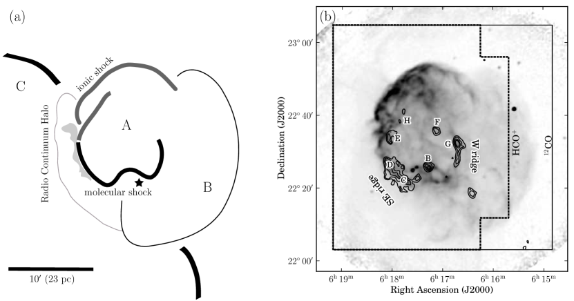
Figure 1.— (a) Schematic showing the overall morphology of IC 443 adopted from LEE08, with the nomenclatures for shells overlaid. The asterisk indicates the position of the pulsar (Olbert et al., 2001). (b) 21cm radio continuum image of IC 443 (LEE08) with the area covered by the FCRAO observations: thin solid polygon for ¹²CO ($J$=1$-$0) and thick dotted polygon for HCO⁺ and HCN. The contours are distribution of shocked ¹²CO (see Fig. 4 for details). The shock clumps (B–H) identified by Denoyer (1979a) and Dickman et al. (1992) are indicated.

Among the known 274 Galactic SNRs (Green, 2009), a few tens of them show direct or indirect evidence of interaction with ambient molecular clouds (see Jiang et al., 2010). IC 443 (G189.1+3.0) is one of the first and most studied SNRs for its interaction with molecular clouds. The overall morphology of IC 443 is depicted in Fig. 1(a). IC 443 has two shells with different radii (Shells A and B, nomenclature is adopted from Braun & Strom, 1986), that are clearly seen in optical and radio continuum images. This peculiar morphology has led to a suggestion that the remnant initially evolved in an inhomogeneous medium. Lee et al. (2008, LEE08 hereafter) suggested that Shell B could be a blowout part of the remnant into a rarefied medium. There is another larger and fainter shell (Shell C) that partially overlaps with Shells A and B. Braun & Strom (1986) proposed that Shell C is also physically associated with Shells A and B, however, the work of Asaoka & Aschenbach (1994) suggests that Shell C is more likely another SNR that is only positionally coincident in the sky .

IC 443 is apparently interacting with both atomic and molecular gas (LEE08, and references therein). The SNR shock in the northeastern part mostly shows the atomic lines expected in postshock recombining gas (Fesen & Kirshner, 1980), and the shock is propagating into an atomic medium. On the other hand, the southern part of the remnant shows shock-excited broad molecular lines, and the SNR shock is encountering molecular clouds (Denoyer, 1979b, a; Burton et al., 1988; Ziurys et al., 1989; Dickman et al., 1992; van Dishoeck et al., 1993). The Two Micron All Sky Survey JHK composite image of Rho et al. (2001) well demonstrates the different nature of the ambient medium.

Shocked molecular gas associated with IC 443 was first discovered in OH and ¹²CO($J$=1$-$0) by Denoyer (1979b, a). Shock acceleration is directly indicated by the large velocity width of the observed lines ($\gtrsim 30\ \mathrm{km\,s}^{-1}$). Broad wings of various molecular lines have been reported (e.g., Ziurys et al., 1989; van Dishoeck et al., 1993) including H₂O (Snell et al., 2005). The overall distribution of shocked molecular gas around IC 443 was mapped by Burton et al. (1988) in H₂, by Dickman et al. (1992) in ¹²CO ($J$=1$-$0) and HCO⁺ ($J$=1$-$0), and by Xu et al. (2011) in ¹²CO ($J$=2$-$1, $J$=3$-$2). Shocked molecular emission is bright along the southern boundary of Shell A, but is also found toward the northeast and near the center of Shell A (Fig. 1(b)). No shocked molecular gas outside Shell A has been reported. The overall distribution of shocked molecular gas has often been described as an expanding ring (Burton et al., 1988; Dickman et al., 1992; van Dishoeck et al., 1993).

On the other hand, the identification and the nature of ambient clouds that are physically interacting with IC 443 have not been comprehensively studied. Ambient molecular clouds toward IC 443 were first reported by Cornett et al. (1977). They found a geometrically thin ($\sim 3$ pc), sheet-like molecular clouds centered around $v_{\mathrm{LSR}}\sim-3\ \mathrm{km\,s}^{-1}$ and proposed its interaction with IC 443. Dickman et al. (1992) published more refined maps of the ambient molecular gas. IC 443 is located toward the Galactic anticenter direction where the radial velocity due to the Galactic rotation is degenerate to $v_{\mathrm{LSR}}\sim 0\,\mathrm{km\,s}^{-1}$. The clouds at $v_{\mathrm{LSR}}\sim-3\ \mathrm{km\,s}^{-1}$ partially overlap with IC 443 in the sky and they are often assumed to be the clouds that are interacting with IC 443 (e.g., Troja et al., 2006), although no clear indication of their physical association has been found.

Identifying the ambient clouds that are physically associated with SNRs is important as it provides fundamental information about the environment of the SNRs. This is particularly important for core-collapse SNRs whose environment is significantly affected by stellar feedback. Also, the study of ambient clouds is important in understanding the hadronic nature of associated $\gamma$-ray emission. $\gamma$-ray emission can be emitted when cosmic rays that are accelerated at SNR shocks encounter nearby dense molecular clouds. IC 443 has long been suspected being a site of cosmic ray acceleration. It harbors an EGRET source 3EG J0617+2238 (Hartman et al., 1999), which might be associated with the hard X-ray source in the eastern boundary (Bykov et al., 2008). A TeV-source in the western boundary is detected by MAGIC (Albert et al., 2007) and VERITAS (Acciari et al., 2009). More recently, GeV emission from IC 443 is reported by Fermi LAT (Abdo et al., 2010) and AGILE (Tavani et al., 2010).

In this paper, we report mapping observations of molecular lines toward the Galactic SNR IC 443. A square-degree field toward IC 443 is mapped in ¹²CO($J$=1–0) and HCO⁺($J$=1–0) with spatial resolution of $\sim 50\arcsec$. Although IC 443 has been observed in various molecular lines, observations have been focused on the broad–line shocked molecular clumps. Our data present a global view of IC 443 and its interaction with molecular clouds. The ¹²CO observations we report here were conducted using the Five College Radio Astronomy Observatory (FCRAO) 14m radio telescope, the same telescope used by Dickman et al. (1992). Dickman et al. mapped IC 443 with full beam spacing (i.e., undersampled), but we obtained fully sampled map using on-the-fly (OTF) technique. The details of observations are described in § 2. Our observations find multiple components of ambient molecular clouds toward IC 443. The characteristics of these multiple cloud complexes are presented in § 3. In § 4, we try to identify ambient clouds that are physically associated with IC 443. The implication of our results on the environment of IC 443 is discussed in § 5 and § 6 summarizes the paper.

2. Observations

A $\sim 1^{\circ}\times 1^{\circ}$ area around IC 443 was observed in ¹²CO  $J$=1–0 (115.2712 GHz) and HCO⁺ $J$=1–0 (89.18852 GHz). All observations were obtained using the FCRAO 14 m telescope during 2003 January. The single sideband 32 element focal plane array receiver SEQUOIA was used in OTF mapping mode. The dual channel correlator (DCC) allowed us to observe two frequencies simultaneously. An area of $60\arcmin\times 62\arcmin$ centered at (06^h17^m00^s, 22$\arcdeg$34$\arcmin$00$\arcsec$) was mapped (Fig. 1) with both channels of DCC set to ¹²CO but at different $v_{\mathrm{LSR}}$, one at $v_{\mathrm{LSR}}=-45$ $\mathrm{km\,s}^{-1}$ and the other at $35$ $\mathrm{km\,s}^{-1}$. A smaller area of $48\arcmin\times 61\arcmin$ centered at (06^h17^m26^s, 22$\arcdeg$34$\arcmin$08$\arcsec$) was mapped with two channels of DCC set to HCO⁺ and HCN at $v_{\mathrm{LSR}}=-15$ $\mathrm{km\,s}^{-1}$, respectively. In this paper, however, we focus on the ¹²CO and HCO⁺ data as the interpretation of the HCN data is complicated due the complexity of its hyperfine structure. The FWHM beam-size of the FCRAO telescope is $\sim 45\arcsec$ at 115 GHZ and $\sim 55\arcsec$ at 89 GHz. The OTF data are regridded on a regular grid of 15$\arcsec$ pixels. The DCC has a bandwidth of 50 MHz and 1024 spectral channels per IF channel, leading to velocity resolution after Hanning smoothing of $0.254$ and $0.328$ $\mathrm{km\,s}^{-1}$ at 115 GHz (CO) and 89 GHz (HCO⁺), respectively. For ¹²CO, the velocity coverages were $-110\ \mathrm{km\,s}^{-1}$ to $+20\ \mathrm{km\,s}^{-1}$, and $-30\ \mathrm{km\,s}^{-1}$ to $+100\ \mathrm{km\,s}^{-1}$ for each channel of the DCC. Previous studies detected emission extending up to $+30\ \mathrm{km\,s}^{-1}$ in the positive velocity and down to $-100\ \mathrm{km\,s}^{-1}$ in the negative velocity (Snell et al., 2005, and references therein). Our observations may not provide adequate velocity coverage for this very high velocity gas. We find that the lack of baseline is severe in some locations for the positive velocity DCC channel data, while negligible for the negative velocity DCC channel data. As the negative DCC channel data cover virtually all the interesting velocity range (see Section  3), we primarily use the negative channel data. For HCO⁺, the velocity coverage was $-100\ \mathrm{km\,s}^{-1}$ to $+70\ \mathrm{km\,s}^{-1}$. The characteristic rms noise of each spectral channel is $\sim 0.2$ K for ¹²CO, and $\sim 0.5$ K for HCO⁺. All the plotted data in this paper are in antenna temperature ($T_{\mathrm{A}}^{*}$), which may be converted to brightness temperature by dividing by the main beam efficiency which is 0.45 and 0.50 at 115 GHz and 90 GHz, respectively. In Fig. 1, we overlay the areas we observed on top of the 21 cm radio continuum image of IC 443 (LEE08).

3. Results

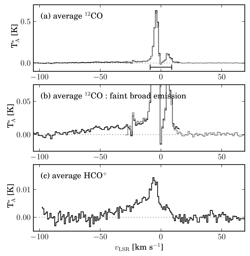
Figure 2.— (a) Average ¹²CO ($J$=1–0) spectra of entire field observed. Two spectra, one centered at $v_{\mathrm{LSR}}$=$-45$ $\mathrm{km\,s}^{-1}$ and the other at $v_{\mathrm{LSR}}$=35 $\mathrm{km\,s}^{-1}$, are shown. The velocity range for channel maps in Fig. 5 is marked. The bump around $-25$ $\mathrm{km\,s}^{-1}$ is an artifact due to an incomplete sky subtraction. (b) Same as (a) but $y$-range is adjusted to show the faint broad lines. (c) Average HCO⁺ spectra of entire field observed. Note that the temperature scale is different.

The spectra of ¹²CO and HCO⁺ lines averaged over the entire observed field are shown in Fig. 2. Most of the CO emission arises from two narrow velocity components at approximately $-3$ $\mathrm{km\,s}^{-1}$ and $+5$ $\mathrm{km\,s}^{-1}$, presumably from ambient molecular cloud. However very weak and broad emission from the shocked gas can also be seen. The average HCO⁺ spectra are dominated by broad lines from the shocked gas. The average spectrum of ¹²CO in Fig. 2 shows an artifact around $v_{\mathrm{LSR}}$= $-20$ $\mathrm{km\,s}^{-1}$, which is the velocity of atmospheric line and we attribute this artifact to an imperfect sky subtraction. This artifact is only seen in the average spectrum and has negligible effect on individual ¹²CO spectra.

3.1. Shocked Molecular Gas

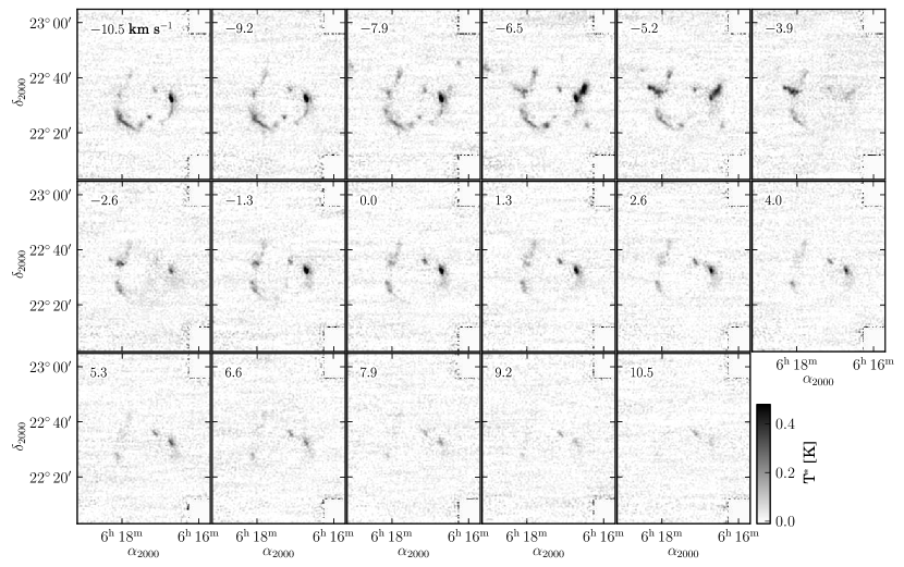
Figure 3.— HCO⁺ channel maps for velocities between $-10$ $\mathrm{km\,s}^{-1}$ and $+10\ \mathrm{km\,s}^{-1}$. The emission is predominantly from shocked molecular gas. However, there is some contribution from the ambient clouds, as can be identified by narrow lines in the PV map (Fig. 4).

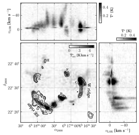
Figure 4.— HCO⁺ integrated temperature map on the lower-left panel, and position-velocity maps on the upper and right panels. The upper panel is an R.A.–velocity map of peak temperatures along the decl. axis. The right panel is a velocity–decl. map of peak temperatures along the R.A. axis. The values are derived from the whole velocity range. The HCO⁺ integrated temperature map has an rms error of 0.3 K$\,\mathrm{km\,s}^{-1}$. The R.A.–velocity map and the velocity–decl. map has an rms error of $0.03$ K. The contours represent ¹²CO integrated temperature map over velocity ranges of $-17$ to $-10$ $\mathrm{km\,s}^{-1}$ and $+1$ to $+3$ $\mathrm{km\,s}^{-1}$, chosen to minimize the contribution from the ambient gas. The contour levels are 1.2, 2.6, 6, 10 K$\,\mathrm{km\,s}^{-1}$ and the rms error is $0.3$ K$\,\mathrm{km\,s}^{-1}$. The shocked clumps are also indicated as in Fig. 1(b). Some HCO⁺ emission is from the ambient gas as can be identified from their narrow line widths. These ambient gas components are associated with the small clouds (see § 3.3).

The shocked molecular gas is characterized by its broad line wings (see Snell et al., 2005, and references therein). For $v_{\mathrm{LSR}}$ $<-10$ $\mathrm{km\,s}^{-1}$ and $v_{\mathrm{LSR}}$ $>+10$ $\mathrm{km\,s}^{-1}$, the emission is confined spatially to small regions with linewidths that are very broad. This emission is assumed to arise almost entirely from the shocked gas. Due to projection effects, the velocity of some of the shocked gas is close to 0 $\mathrm{km\,s}^{-1}$ (Dickman et al., 1992) and a significant fraction of the shocked gas is indeed in the velocity range between $v_{\mathrm{LSR}}$$=-10$ to $+10$ $\mathrm{km\,s}^{-1}$. But the study of this low velocity shocked gas with ¹²CO is difficult due to the contamination by the ambient gas emission (Fig. 2). HCO⁺ emission, on the other hand, has less contamination from the ambient gas. The channel maps and the position-velocity (PV) maps of the observed HCO⁺ line are shown in Fig. 3 and in Fig. 4. In particular, the PV maps clearly show that most of the emission has a line width $\gtrsim 10\ \mathrm{km\,s}^{-1}$, and thus is from the shocked gas. Some ambient gas is picked up as absorption features and also as emission features. Thus HCO⁺ is better suited for studying the overall distribution of the shocked molecular gas. In Fig. 4, the distribution of high-velocity ¹²CO emission is compared to the distribution of HCO⁺ emission. We note that the ¹²CO image at higher velocity can provide more sensitive and detailed distribution of shocked gas compared to HCO⁺ data with a caveat that the lower velocity shocked gas is not included.

The distribution of shocked molecular gas takes a shape of an incomplete ring, which consists of several bright clumps and fainter emission that seems to connect these clumps. The shocked gas emission is brighter in the south, while the emission in the north is weaker. There is a general tendency of the systematic velocity of shocked gas getting more positive with the increasing declination. This large-scale velocity gradient is consistent with previous studies which suggested that the large-scale distribution of the shocked gas in IC 443 could be described as an expanding ring (Burton et al., 1988; Dickman et al., 1992). On the other hand, we note that long ($\gtrsim$ a few arcminutes) filaments of shocked gas are only prominent in the southeastern (SE ridge) and western parts (W ridge) of the proposed ring (Figure 4) and the gas kinematics are dominated by rapid variation on the scale of $\lesssim$ a few arcminutes, which are referred as shocked “clumps”. The PV plot in right ascension (the top panel of Fig. 4) shows a tilt of the emission in clumps B and C. In clump B, the emission shifts to smaller R.A. at higher shock velocities, while for clump C, the emission shifts to larger R.A. at higher shock velocities. Little shift is seen in the PV plot in declination. The velocity shift seen in Clump B was first detected by Dickman et al. (1992) in both ¹²CO and HCO⁺ emission. They suggested that this shift was a sign that the gas was being ablated and accelerated away from the shocked clump. It is interesting that we see a similar effect in Clump C, although the ablated gas is moving off in the opposite direction. Although the geometry of the interaction of the SNR with the ambient gas is complicated, these tilts in the PV diagram provide an indication of the direction of the shock.

3.2. Ambient Molecular Gas

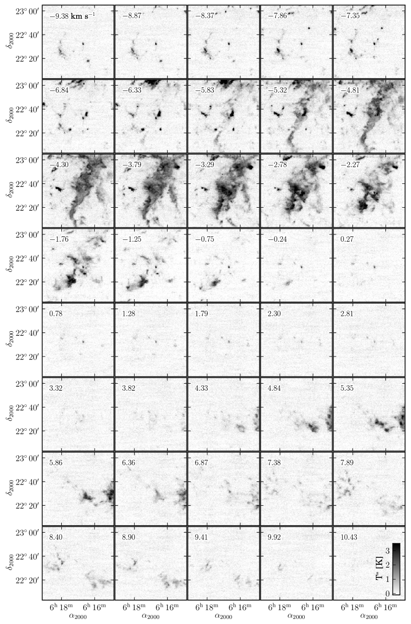
Figure 5.— ¹²CO channel maps for velocities between $-10$ $\mathrm{km\,s}^{-1}$ and $+10\ \mathrm{km\,s}^{-1}$, mostly tracing the ambient molecular gas. Each panel represents mean temperature for $\Delta v=0.5\ \mathrm{km\,s}^{-1}$, where their central velocity is shown in the top-left corner.

The channel maps of ¹²CO in the velocity range of $v_{\mathrm{LSR}}$= $-10$ $\mathrm{km\,s}^{-1}$ to $+10$ $\mathrm{km\,s}^{-1}$, where most of the emission traces ambient clouds, are shown in Fig. 5. IC 443 is located toward the Galactic anticenter direction, and no ambient molecular gas emission is found outside of this velocity range. The channel maps in Fig. 5, together with the mean ¹²CO spectrum in Fig. 2, suggest that there are two distinct complexes of molecular gas, one in the negative velocity of $-10\ \mathrm{km\,s}^{-1}<v_{\mathrm{LSR}}<0\ \mathrm{km\,s}^{-1}$ and the other in the positive velocity of $+3\ \mathrm{km\,s}^{-1}<v_{\mathrm{LSR}}<+10\ \mathrm{km\,s}^{-1}$.

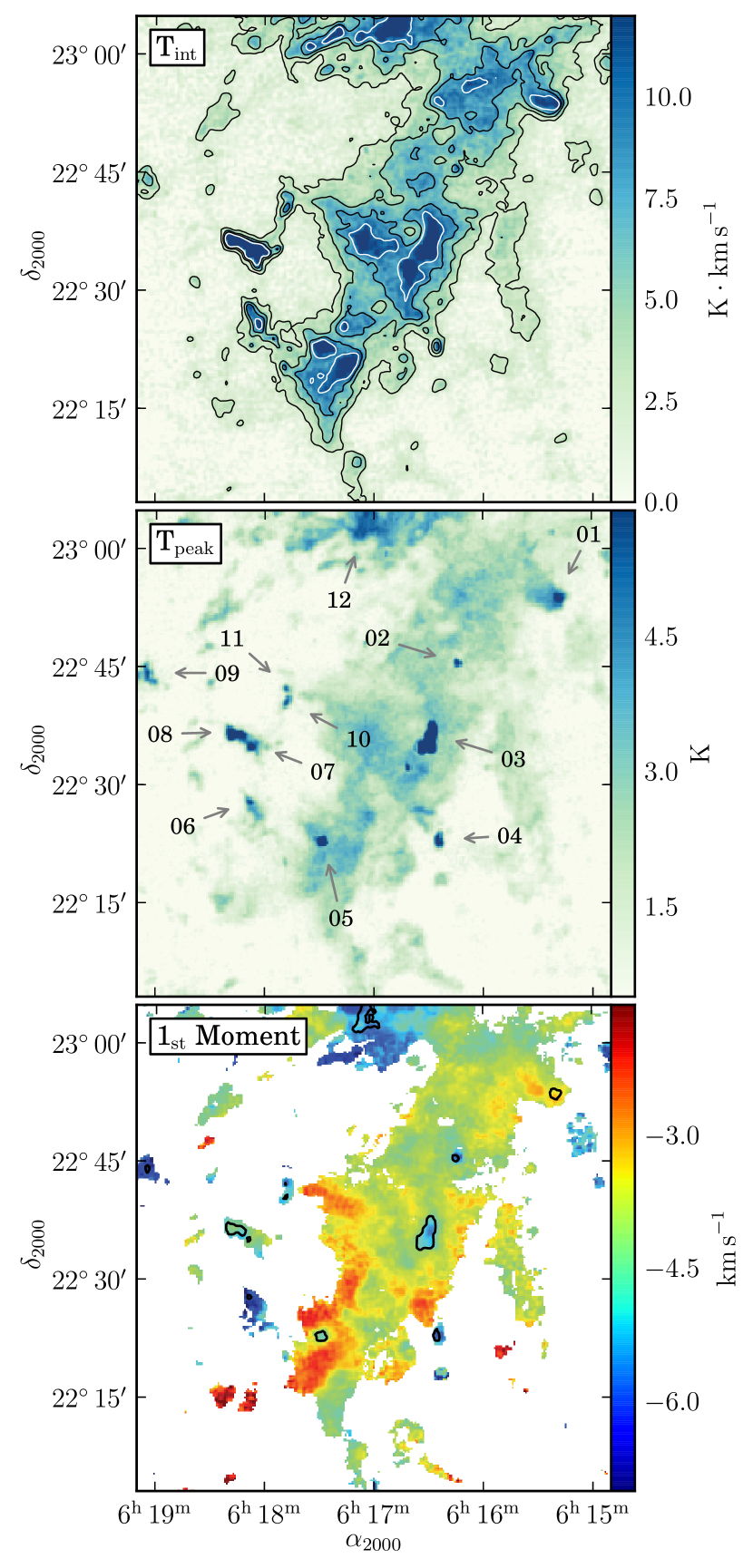
Figure 6.— (a) ¹²CO integrated temperature map in velocity range of $-10$ to $0\ \mathrm{km\,s}^{-1}$, mostly tracing the ambient gas. (b) ¹²CO peak temperature map over the same velocity interval. The numbers denote the location of small clouds (SCs) discussed in § 3.3. (c) The intensity weighted mean velocity (first moment) of the ¹²CO emission. The contours mark the regions which satisfy our selection criteria for SCs (see § 3.3 for details).

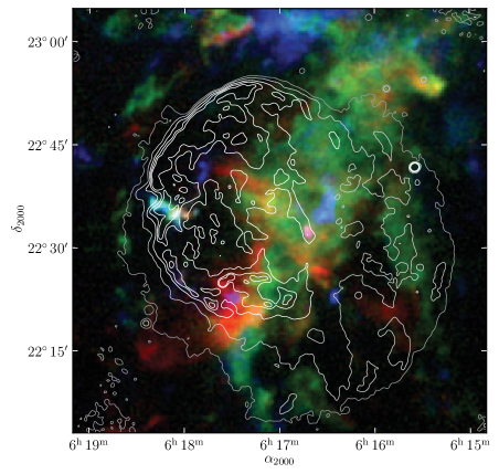
Figure 7.— RGB composite image where each R, G, and B channel corresponds to ¹²CO integrated temperature maps of velocity ranges $-0.5$ to $-3.4$, $-3.4$ to $-5.1$ and $-5.1$ to $-7.0\ \mathrm{km\,s}^{-1}$, respectively. The contours are 21cm radio continuum image from LEE08. The contour levels are 10, 20, 40, 60, 80 mJy.

The clouds at negative velocities show significant channel-to-channel variation. To get a grasp of the overall structure of the cloud complex, we generate an integrated temperature map, a peak temperature map and a first moment (intensity weighted velocity) map of ¹²CO emission in the velocity range $-10<v_{\mathrm{LSR}}<0\ \mathrm{km\,s}^{-1}$, which are shown in Fig. 6. Also, in Fig. 7, an RGB composite image is shown, where each red, green and blue channel corresponds to an integrated temperature map of different velocity ranges (see the figure caption for more details). The integrated temperature map provides an overall view of the spatial distribution of this gas, although there is some contamination by emission from the shocked gas. Most of the ambient gas is distributed along the northwest-southeast direction across the field, roughly corresponding to the interface between Shells A and B (Fig. 7). The peak temperature map is similar to the integrated temperature map, however, several small clouds ($\sim 1\arcmin$) with relatively higher peak temperatures ($\gtrsim$ 5 K) stand out against the diffuse clouds whose peak temperatures are generally less than 3 K. These small clouds are even more prominent in the PV maps in Fig. 8. Fig. 8 clearly reveals two distinguished kinematic characteristics of the small clouds compared to the diffuse clouds. First, the linewidths of these small clouds are much narrower than the diffuse clouds. Second, most of these small clouds show clear offset in velocity relative to the diffuse emission. Although some of these small clouds are located toward the diffuse clouds, a significant velocity offset between them suggests that most of the small clouds are not related to the diffuse clouds. Thus, these small clouds are considered to be separate clouds from the diffuse clouds. For the purpose of the discussion, we denote the diffuse clouds between $-6\ \mathrm{km\,s}^{-1}$ and $-1\ \mathrm{km\,s}^{-1}$ as “$-3\ \mathrm{km\,s}^{-1}$ clouds” and the small high brightness temperature clouds as “SCs”. The characteristics of the SCs will be further discussed in § 3.3. The first moment map mostly traces the radial velocity variation within the $-3\ \mathrm{km\,s}^{-1}$ clouds and suggests that the main body of the cloud has a small, systematic velocity shift from east to west. A similar tendency can be noticed in the RGB composite image (Fig. 7).

In the positive velocity range, relatively fainter emission from ambient clouds is seen between $v_{\mathrm{LSR}}=+3$ and $+10\ \mathrm{km\,s}^{-1}$. We call these clouds as “$+5\ \mathrm{km\,s}^{-1}$ clouds”. Emission between $0\ \mathrm{km\,s}^{-1}$ and $+3\ \mathrm{km\,s}^{-1}$ is predominantly from shocked molecular gas. Fig. 9 shows integrated temperature map of $v_{\mathrm{LSR}}=+4$ to $+10\ \mathrm{km\,s}^{-1}$, which represent mostly the ambient gas with some contribution of the shocked gas. The clouds seem to be divided into two parts: the western part and the eastern part. The western part is brighter and shows a prominent filamentary structure. The eastern part is fainter and shows a number of small clouds. It is noteworthy that the western and the eastern parts are separated by Shell A (Fig. 9).

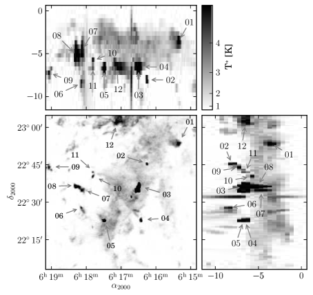
Figure 8.— ¹²CO peak temperatures map (identical to Fig. 6(b)) together with position–velocity maps. The upper panel is a R.A.–velocity map of peak temperatures along the decl. axis. The right panel is a velocity–decl. map of peak temperatures along the R.A. axis. The images are shown in a squared scale to better visualize the locations of the SCs. The numbers are identification numbers for SCs. The central velocities of SCs are adopted from $v_{0}$ of Component 1 in Table 1.

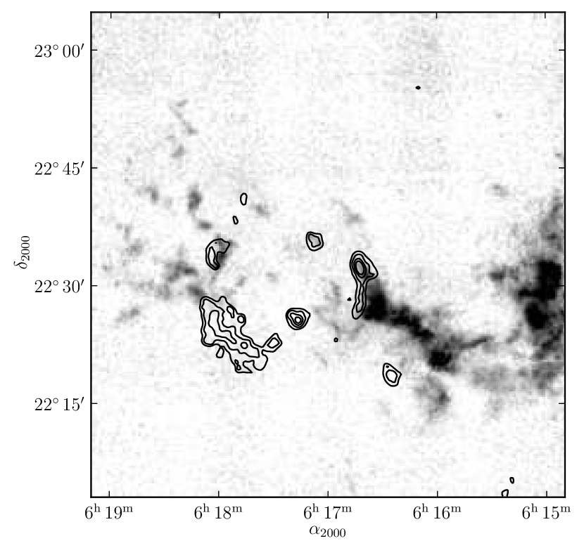
Figure 9.— ¹²CO distribution of $+5\ \mathrm{km\,s}^{-1}$ clouds, integrated over velocity range of $+4\ \mathrm{km\,s}^{-1}$ to $+10\ \mathrm{km\,s}^{-1}$. The contours are ¹²CO integrated temperature map as in Figure 4, tracing the distribution of shocked molecules.

3.3. Small Clouds (SCs)

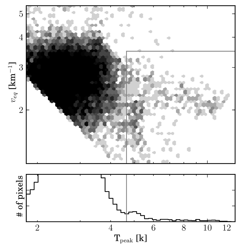
Figure 10.— (top) distribution of $T_{\mathrm{peak}}^{*}$ vs. $\Delta v_{\mathrm{eq}}$ (equivalent line width), where $\Delta v_{\mathrm{eq}}$, defined as $T_{\mathrm{int}}^{*}$/ $T_{\mathrm{peak}}^{*}$. While most pixels have $T_{\mathrm{peak}}^{*}$$\lesssim 4$ K and $\Delta v_{\mathrm{eq}}$ $\sim$ 2 $\mathrm{km\,s}^{-1}$, there are pixels with $T_{\mathrm{peak}}^{*}$$\gtrsim 5$ K and $\Delta v_{\mathrm{eq}}\lesssim$ 3 $\mathrm{km\,s}^{-1}$ which are associated with SCs. The gray lines mark the selection criteria used to identify SCs. (bottom) Histogram of $T_{\mathrm{peak}}^{*}$. A clear bump around 5 K is seen. The gray vertical line marks $T_{\mathrm{peak}}^{*}$=4.6 K above which are necessary condition to be identified as SCs.

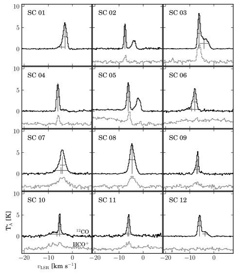
Figure 11.— ¹²CO line profiles of the SCs. The crosses indicate the line center and the full-width-at-half-maximum when fit by multiple Gaussian components (see Table 1). HCO⁺ spectra at the same locations are also shown as gray lines. No HCO⁺ spectrum is available for SC 01 as the observed area for HCO⁺ is smaller than that for ¹²CO.

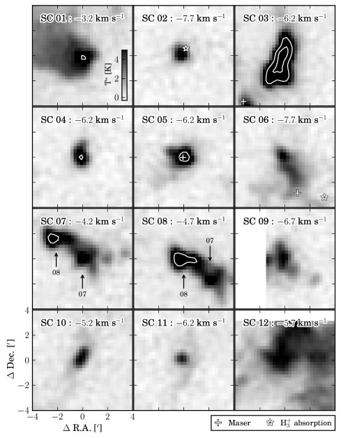
Figure 12.— $8\arcmin\times 8\arcmin$ close-up view of each SC at its peak velocity (see Table 1). Each panel is labeled with the SC number and the channel velocity used. The white contours are $\mathrm{T}^{*}=$ 5 K, 7.5 K and 10 K. The plus signs near SCs 03, 05 and 06 are positions of OH maser sources and the star signs near SC 02 and 06 are sight lines along which H${}_{3}^{+}$ absorption features are detected (see § 4.1). The locations of SC 07 and SC 08 are also marked with arrows for clarification.

The ¹²CO peak temperature map in Fig. 6 and the PV maps in Fig. 8 reveal the existence of several SCs ($\sim 1\ \arcmin$) with relatively high brightness temperature and narrow line width. To identify these clouds in more systematic way, we utilize two characteristic quantities: the peak temperatures ($T_{\mathrm{peak}}^{*}$) and the equivalent line width ($\Delta v_{\mathrm{eq}}$). $\Delta v_{\mathrm{eq}}$ is defined as the ratio of the integrated temperatures $T_{\mathrm{int}}^{*}$ to $T_{\mathrm{peak}}^{*}$. These temperatures are measured in the velocity range of $-10$ $\mathrm{km\,s}^{-1}$ to $0$ $\mathrm{km\,s}^{-1}$. Fig. 10 shows a two dimensional histogram of these two quantities measured from the pixels in the observed area. Most pixels have $T_{\mathrm{peak}}^{*}$$\lesssim 4$ K and $1\lesssim v_{\mathrm{eq}}\lesssim\ 4\ \mathrm{km\,s}^{-1}$, and we find that they are mostly associated with $-3\ \mathrm{km\,s}^{-1}$ clouds. On the other hand, there are pixels with relatively high peak temperature ($T_{\mathrm{peak}}^{*}$$\gtrsim$ 4.5 K) with relatively narrower equivalent line width ($v_{\mathrm{eq}}\lesssim 3\ \mathrm{km\,s}^{-1}$). We find these pixels correspond to the SCs as suspected. Based on the two-dimensional histogram, we adopt a criteria of $T_{\mathrm{peak}}^{*}$$>$ 4.6 K and $v_{\mathrm{eq}}<3.5\ \mathrm{km\,s}^{-1}$, which results in the identification of 12 SCs, and these are identified in Fig. 6(b) and labeled with numbers (e.g., SC 01). The selection process includes all of the SCs that would have been chosen by eye, as we are primarily selecting them based on peak temperature.

The ¹²CO line profiles of the 12 SCs are shown in Fig. 11. These are average spectra extracted from the contours shown in Fig. Fig. 6(b), and they all show narrow lines with high peak temperatures as expected. We fit the spectra with Gaussian profiles and the results are summarized in Table 1. Often, the spectra need multiple Gaussian components to be adequately fit. The additional components are contributed by emission from either the diffuse clouds or the shocked gas.

Central velocities of these SCs range between $-3$ and $-8\,\mathrm{km\,s}^{-1}$, with a median of $\sim-6\,\mathrm{km\,s}^{-1}$. Other than SC 01, 07/08 (see the note in Table 1), they have peak velocities more negative than $-5\ \mathrm{km\,s}^{-1}$, and are well separated from $-3\ \mathrm{km\,s}^{-1}$ clouds in the velocity space (Fig. 8). Their line widths are between $1$ and $2\ \mathrm{km\,s}^{-1}$. The HCO⁺ profiles are also plotted in Fig. 11 when available. The SCs tend to have similar narrow emission lines in HCO⁺. The ¹²CO maps of $\sim 8\arcmin\times 8\arcmin$ regions around individual SCs at their peak intensity channels are shown in Fig. 12. Part of the emission seen around SCs 05, 06, 07/08, 10, and 11 is due to shocked gas, and the association of these SCs to the shocked molecular gas will be further discussed in § 4.1.

Table 1Spectral parameters of the small clouds (SCs; see § 3.3)

			Component 1				Component 2
SC No.	$\alpha$ (2000)	$\delta$ (2000)	T${}_{\mathrm{A}}^{*}$ [K]	$v_{0}$	$v_{\mathrm{FWHM}}$		T${}_{\mathrm{A}}^{*}$ [K]	$v_{0}$	$v_{\mathrm{FWHM}}$
01	06h15m20$\fs$1	22$\arcdeg$53$\arcmin$43$\arcsec$	5.7 $\pm$ 0.5	-3.1 $\pm$ 0.1	1.6 $\pm$ 0.1		0.9 $\pm$ 0.3	-4.6 $\pm$ 0.5	2.7 $\pm$ 0.6
02	06h16m14$\fs$4	22$\arcdeg$45$\arcmin$14$\arcsec$	6.0 $\pm$ 0.1	-7.5 $\pm$ 0.1	0.9 $\pm$ 0.1
03	06h16m29$\fs$6	22$\arcdeg$36$\arcmin$14$\arcsec$	7.3 $\pm$ 0.1	-6.2 $\pm$ 0.1	1.2 $\pm$ 0.1		2.6 $\pm$ 0.1	-4.1 $\pm$ 0.1	3.6 $\pm$ 0.1
04	06h16m25$\fs$3	22$\arcdeg$22$\arcmin$44$\arcsec$	6.6 $\pm$ 0.1	-6.0 $\pm$ 0.1	1.2 $\pm$ 0.1		0.5 $\pm$ 0.1	-3.5 $\pm$ 0.1	2.0 $\pm$ 0.2
05	06h17m29$\fs$1	22$\arcdeg$22$\arcmin$44$\arcsec$	6.7 $\pm$ 0.1	-6.2 $\pm$ 0.1	1.3 $\pm$ 0.1
06	06h18m08$\fs$1	22$\arcdeg$27$\arcmin$44$\arcsec$	4.4 $\pm$ 0.2	-7.9 $\pm$ 0.1	1.5 $\pm$ 0.1		0.9 $\pm$ 0.1	-9.2 $\pm$ 0.2	5.2 $\pm$ 0.3
07	06h18m08$\fs$2	22$\arcdeg$34$\arcmin$58$\arcsec$	4.1 $\pm$ 0.3	-4.1 $\pm$ 0.1	2.2 $\pm$ 0.1		1.6 $\pm$ 0.1	-4.7 $\pm$ 0.1	5.4 $\pm$ 0.3
08	06h18m17$\fs$9	22$\arcdeg$36$\arcmin$28$\arcsec$	6.6 $\pm$ 0.1	-4.6 $\pm$ 0.1	2.4 $\pm$ 0.1
09	06h19m04$\fs$6	22$\arcdeg$43$\arcmin$57$\arcsec$	3.5 $\pm$ 0.4	-6.7 $\pm$ 0.1	0.7 $\pm$ 0.1		2.1 $\pm$ 0.2	-7.1 $\pm$ 0.1	1.7 $\pm$ 0.1
10	06h17m48$\fs$7	22$\arcdeg$40$\arcmin$14$\arcsec$	4.6 $\pm$ 0.2	-5.3 $\pm$ 0.1	0.7 $\pm$ 0.1		1.0 $\pm$ 0.1	-6.4 $\pm$ 0.1	7.0 $\pm$ 0.3
11	06h17m48$\fs$7	22$\arcdeg$41$\arcmin$59$\arcsec$	4.0 $\pm$ 0.5	-6.0 $\pm$ 0.1	0.9 $\pm$ 0.1		1.1 $\pm$ 0.2	-6.4 $\pm$ 0.1	2.3 $\pm$ 0.3
12	06h17m06$\fs$5	23$\arcdeg$01$\arcmin$45$\arcsec$	5.0 $\pm$ 0.1	-6.0 $\pm$ 0.1	1.4 $\pm$ 0.1		1.1 $\pm$ 0.1	-3.7 $\pm$ 0.1	2.1 $\pm$ 0.1

Note. — The velocities are in $\mathrm{km\,s}^{-1}$.

Note. — SCs 07 and 08 are positionally close and have similar systematic velocities, and they will be labeled together as SCs 07/08 when necessary.

4. Identification of Ambient Clouds Interacting with IC 443

The shocked molecular gas in IC 443 is mostly found within Shell A. No shocked molecular gas has been identified outside Shell A (Dickman et al., 1992), even with our new wide-field, fully-sampled mapping observations. The signature of the shocked molecular gas is prominent along the southern boundary of Shell A (e.g., Burton et al., 1988). On the other hand, the nature of the ambient molecular clouds that are associated with shocked molecular gas in IC 443 has not been clearly understood. Our observations reveal the existence of three different cloud complexes ($-3\ \mathrm{km\,s}^{-1}$ clouds, SCs and $+5\ \mathrm{km\,s}^{-1}$ clouds) toward IC 443. Here we investigate possible association of these cloud complexes with IC 443.

4.1. SCs

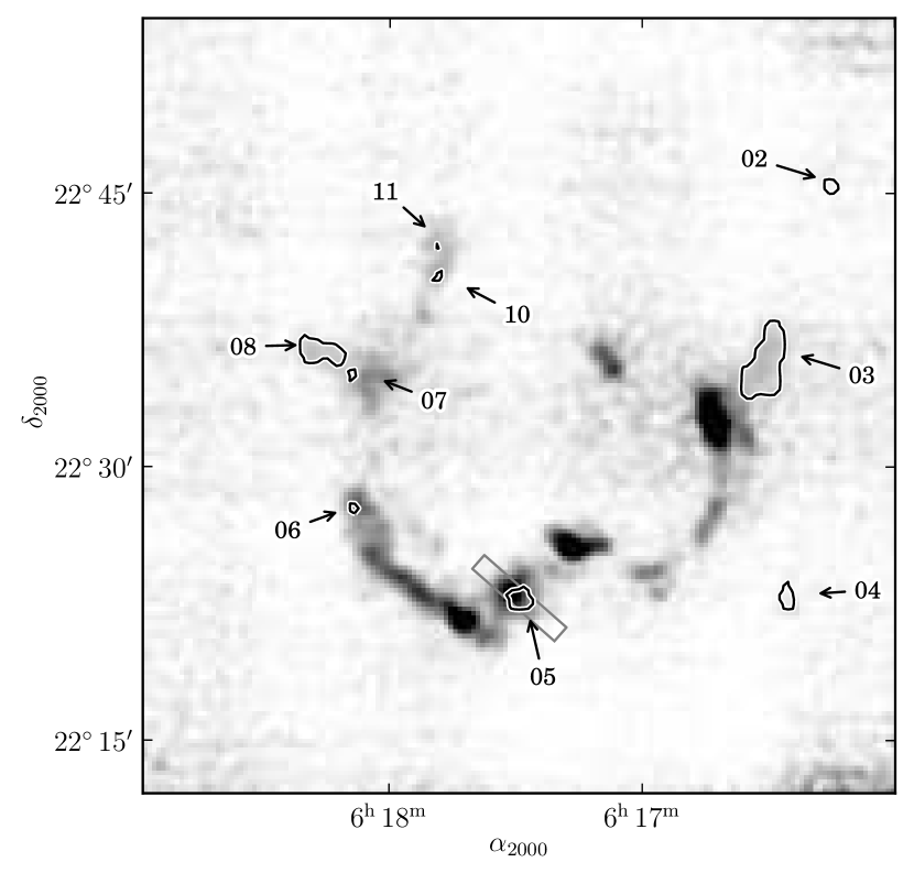
Figure 13.— Locations of the SCs overlaid over the average temperature map of HCO⁺. The gray rectangle is the extraction area for the PV map in Fig. 14.

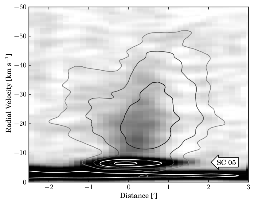
Figure 14.— PV map of ¹²CO emission around SC 05 extracted from the slit in Fig. 13. The distance is measured from the location of SC 05 and the value increases with increasing right ascension. The contours represent a PV map of HCO⁺ extracted from the same slit. The location of SC 05 in the PV map (distance $\sim$ 0′, $v_{\mathrm{LSR}}\sim-6$ $\mathrm{km\,s}^{-1}$) is marked.

The SCs around IC 443 are identified for the first time in our observations. We find that their spatial distribution is closely related to the distribution of shocked gas in IC 443. In Fig. 13, we overlay the locations of the SCs on top of the distribution of the shocked molecular gas. The positions of SCs 05, 06, 10, and 11 are coincident with those of the shocked molecular clumps. Also, the southeastern tip of SC 03 is coincident with Clump G, and the southwestern tip of SCs 07/08 with Clump E (we note that these SCs are spatially more extended than those regions defined by our selection criteria). While some of the positional coincidence could be by chance, the fact that a large fraction of the SCs shows their projected positions on the sky being coincident with those of shocked clumps suggests that they are more likely physically associated.

Evidence of the physical association of the SC’s with the shocked molecular gas is best seen in SC 05. Fig. 14 shows PV maps of ¹²CO and HCO⁺ along an NE–SW direction and the location of this PV cut is indicated in Fig. 13. The spatial extent of the shocked gas is nearly identical to that of SC 05, unlike the emission from the more spatially extensive $-3\ \mathrm{km\,s}^{-1}$ clouds. This coincidence strongly suggests that SC 05 is physically related to the shocked gas.

We further find that the locations of the three OH 1720 MHz maser sources currently known in IC 443 are spatially close to the SCs or even coincident (Fig. 12). Furthermore, the systematic velocity of the maser source in SC 05 ($-6.1\pm 0.1\ \mathrm{km\,s}^{-1}$, Hewitt et al., 2006) is coincident with the systematic velocity of SC 05 itself. The velocity of the maser source near SC 06 ($-6.9\pm 0.1\ \mathrm{km\,s}^{-1}$, Hewitt et al., 2006) is also in agreement with the velocity of SC 06. The velocity of the source near SC 03 (the source that is coincident with Clump G) is $-4.55\ \mathrm{km\,s}^{-1}$ (Hewitt et al., 2006). While this is slightly different from the peak velocity of SC 03, it is still within the velocity wing of SC 03. We consider that this maser source could be associated with SC 03.

Recently, Indriolo et al. (2010) searched for H${}_{3}^{+}$ absorption features in six sight lines towards IC 443. From the absorption features seen in two sight lines, high ionization rates are inferred which are attributed to the increased cosmic ray ionization rate near IC 443. The two sight lines with high ionization rates are indeed located close to the SCs (see Fig. 12). The centroid velocities of the absorption features are between $-8$ and $-6\ \mathrm{km\,s}^{-1}$, being consistent with the velocity range of the SCs.

Therefore, we found that a good fraction of the SCs show direct and/or indirect association with the shocked molecular clumps. We propose that the SCs are at the same distance as IC 443, and that some of them are in direct interaction with IC 443.

4.2. $+5\ \mathrm{km\,s}^{-1}$ clouds

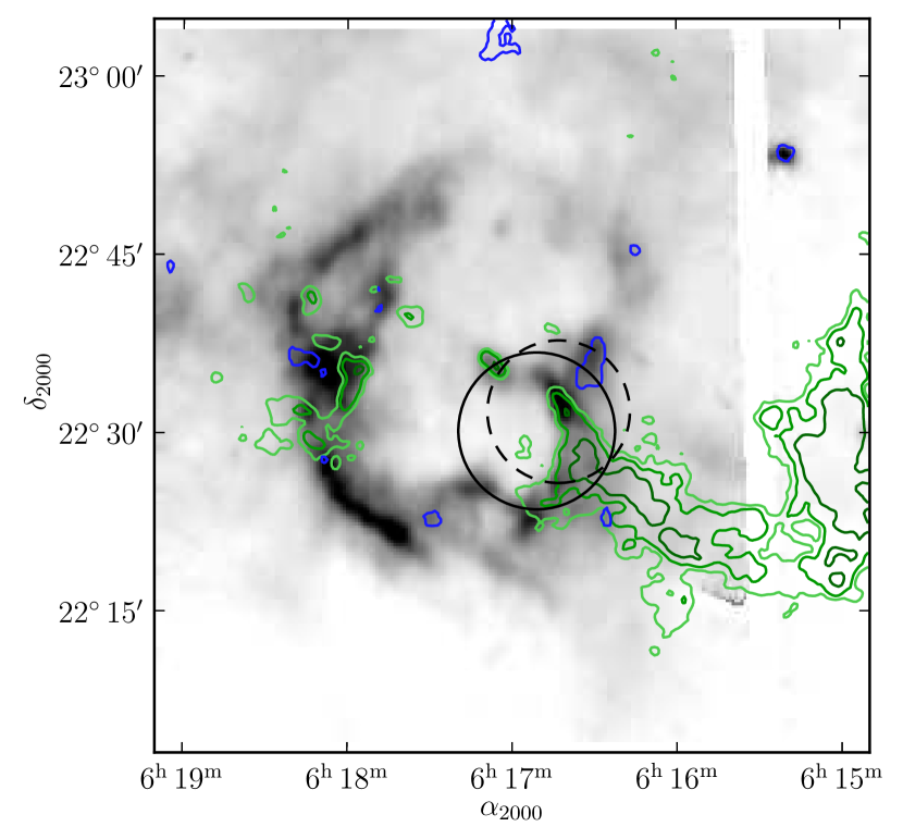
Figure 15.— Far IR 90 $\mu$m image taken with the AKARI satellite shown in gray scale. The green contours show the distribution of $+5\ \mathrm{km\,s}^{-1}$ clouds (the gray scale in Fig. 9). The blue contours show locations of SCs. The solid and dashed circles represent the location of $\gamma$-ray sources detected by MAGIC and VERITAS, respectively.

The detailed morphology of $+5\ \mathrm{km\,s}^{-1}$ clouds is also newly revealed in our observations. The overall morphology of the clouds, which is shown in Fig. 9, is intriguing. As has been previously described, the clouds can be divided into two parts. The brighter western part has a prominent filamentary morphology. It extends from west to east. Its eastern boundary is sharp and we see a filament of shocked gas along this boundary (clump G and W ridge). In Fig. 15, we compare the morphology of $+5\ \mathrm{km\,s}^{-1}$ clouds to that of 90 $\mu$m far infrared emission from IC 443. The far infrared emission, taken by AKARI telescope, is presumably from the shock heated dust and defines the outer boundary of Shell A. Interestingly, the $+5\ \mathrm{km\,s}^{-1}$ clouds (both the western and the eastern parts) are only visible along and/or outside Shell A. Therefore, there is a good morphological coincidence between the $+5\ \mathrm{km\,s}^{-1}$ clouds and the shock tracers.

On the other hand, the systematic velocity of the shocked gas in Clump G and the W ridge is around $-5\ \mathrm{km\,s}^{-1}$, and thus is considerable offset from that of the $+5\ \mathrm{km\,s}^{-1}$ clouds. The symmetric line profile of Clump G suggests that the shock direction is mostly perpendicular to our line-of-sight, thus shock geometry is unlikely to explain the 10 $\mathrm{km\,s}^{-1}$ difference in radial velocity. Can these kinematically distinct clouds be adjacent in space? IC 443 is likely a core-collapse SNR located in the Gem OB1 association (Braun & Strom, 1986), and there could be clouds with different velocities due to the complicated kinematics within this OB association. However, the difference of $10$ $\mathrm{km\,s}^{-1}$ seems to require rather extraordinary condition. Therefore, while the morphology of the $+5\ \mathrm{km\,s}^{-1}$ clouds is rather suggestive of its association with IC 443, there is no kinematic evidence that these $+5\ \mathrm{km\,s}^{-1}$ clouds are responsible for any of the shocked molecular gas. We do not consider that the physical association of the $+5\ \mathrm{km\,s}^{-1}$ clouds with IC 443 is conclusive.

4.3. $-3\ \mathrm{km\,s}^{-1}$ clouds

The $-3\ \mathrm{km\,s}^{-1}$ clouds show elongated morphology in the NW–SE direction, along the interface between Shells A and B. There is supporting evidence that most of these clouds are located on the front side of the remnant (Troja et al., 2006, and references therein), and the self-absorption features in ¹²CO and HCO⁺ (van Dishoeck et al., 1993) are consistent with this conclusion. Thus, any interaction of IC 443 with these clouds would likely produce blueshifted gas; however, we see both redshifted and blueshifted shocked gas. Also, we see little correlation between the locations of the shocked gas and the spatial distribution of the $-3\ \mathrm{km\,s}^{-1}$ clouds. While the velocity gradient within the $-3\ \mathrm{km\,s}^{-1}$ clouds might be due to some external perturbation, we could not find any hint that this is due to the interaction with IC 443 or its progenitor star. An OH 1720 MHz maser source associated with Clump G has a systematic velocity of $-4.55$ $\mathrm{km\,s}^{-1}$ (Hewitt et al., 2006), comparable to the velocity of $-3\ \mathrm{km\,s}^{-1}$ clouds. However, the location and the velocity of the maser source are also consistent with those of SC 03, so the association of this maser source with the $-3\ \mathrm{km\,s}^{-1}$ clouds is considered ambiguous. We find no strong evidence for a spatial or kinematic connection between the shocked gas and the $-3\ \mathrm{km\,s}^{-1}$ clouds, thus we conclude that the remnant is not currently interacting with the $-3\ \mathrm{km\,s}^{-1}$ clouds.

5. Discussion

5.1. Origin of the Small Clouds & Environment of IC 443

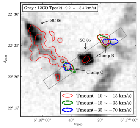
Figure 16.— Gray scale shows a peak temperature map of ¹²CO in velocity range $-0.2$ and $-5.4$ $\mathrm{km\,s}^{-1}$, mostly representing the ambient gas. Red, green, and blue contours are integrated temperatures of ¹²CO for velocity range of $-10$ to $-15$ $\mathrm{km\,s}^{-1}$, $-15$ to $-35$ $\mathrm{km\,s}^{-1}$, and $-35$ to $-70$ $\mathrm{km\,s}^{-1}$, respectively. They show emission from shocked molecular gas. The long rectangles are extraction regions for the PV maps in Fig. 17.

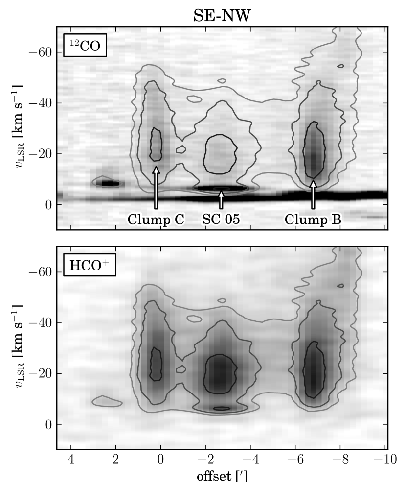
Figure 17.— PV maps along the slit shown in Fig. 16. The upper panel is for ¹²CO, and the lower panel is for HCO⁺. The gray contours, both in upper and lower panels, are those of HCO⁺. The offsets are distance in arcminute measured from Clump C (marked as a plus sign in Fig. 16) and the offset increases with increasing right ascension.

Table 2H₂ column densities and masses of SCs.

SC#	H2 Column Density	Mass
	[$\times 10^{21}$ cm-2]	[${M}_{\odot}$]
01	$4.3\pm 0.5$	$12.6\pm 1.6$
02	$2.5\pm 0.1$	$\phantom{0}3.5\pm 0.1$
03	$4.0\pm 0.1$	$57.7\pm 0.9$
04	$3.6\pm 0.1$	$\phantom{0}7.0\pm 0.1$
05	$4.1\pm 0.1$	$13.2\pm 0.2$
06	$3.0\pm 0.2$	$\phantom{0}2.0\pm 0.1$
07	$4.2\pm 0.4$	$\phantom{0}2.7\pm 0.3$
08	$7.4\pm 0.1$	$85.8\pm 0.7$
09	$1.2\pm 0.2$	$\phantom{0}1.2\pm 0.2$
10	$1.5\pm 0.1$	$\phantom{0}0.8\pm 0.1$
11	$1.7\pm 0.3$	$\phantom{0}0.4\pm 0.1$
12	$3.2\pm 0.5$	$36.9\pm 0.7$

Note. — H₂ column densities are estimated from the fit parameters of component 1 in Table 1. We corrected for the main beam efficiency and adopted the canonical conversion factor X ($\equiv N_{\mathrm{H}_{2}}/\int{T(^{12}\mathrm{CO})dv}$) of $\sim 2\times 10^{20}$ cm^-2K^-1km^-1s (e.g., Dame et al., 2001). To estimate the mass, we multiply the H₂ mass by a factor of 1.36 to account for the mass of helium. The errors in this table are formal errors from the spectral fit and do not include any systematic error.

The physical characteristics of the SCs, size of $\sim 0.5$ pc ($\sim 1\arcmin$ at 1.5 kpc) and velocity dispersion of $\sim 1\ \mathrm{km\,s}^{-1}$, resemble small clumps in molecular clouds (cf., Bergin & Tafalla, 2007). We estimate the hydrogen column density of SCs using the canonical conversion factor X ($\equiv N_{\mathrm{H}_{2}}/\int{T(^{12}\mathrm{CO})dv}$) of $\sim 2\times 10^{20}$ cm^-2K^-1km^-1s (e.g., Dame et al., 2001), and list these in Table 2. If we assume a path length of $\sim 0.5$ pc (1$\arcmin$, which is a typical angular diameter of the SCs, at a distance of 1.5 kpc), we obtain average molecular hydrogen densities of the order of $10^{3}$ $\rm{cm}^{-3}$ (higher densities must be present to produce the HCO⁺ emission seen in most of the SCs, suggesting that the clouds could be clumped and have a small filling factor within the beam). The masses of the individual clouds are estimated to be of order of $10$ ${M}_{\odot}$ (Table 2). This is comparable to the mass of individual shocked clumps (5–40 ${M}_{\odot}$; Dickman et al., 1992), and also comparable to that of small clumps (cf., Bergin & Tafalla, 2007).

One of the key characteristics of the SCs is that they lack surrounding clouds. We propose that the SCs are analogous to the cometary globules, i.e., remnant cores of molecular clouds that have been exposed as their lower density gas envelopes have been removed by the prior activity of the SN progenitor star or nearby OB stars (Reipurth, 1983). For SCs 01 and 12, located farther from IC 443, the removal of lower density envelopes may have not been complete as we see some diffuse ambient gas around them. Some of the SCs are now being impacted by the SNR and the gas is being ablated and accelerated producing the shocked molecular clumps (e.g., SC 05 and the associated shocked gas). The interaction of small clouds with shock waves have been comprehensively studied by numerical simulations (e.g., Klein et al., 1994). Upon interaction, transmitted shocks will propagate into the cloud core and the envelope will be stripped away. This nicely explains the spatio-kinematic structure of the gas around SC 05. In this picture, some part of the core is already shocked and ablated, while the remaining part is yet to be shocked. The ambient gas of SC 05 itself is unperturbed part of the core, and the high velocity gas would represent a flow of gas that is primarily ablated from the core.

In figure 17, we show a PV diagram along a slit extending NW-SE through SC 05 and covers Clumps B and C and SC 05 (see Figure 16 for the location of the slit). It indicates that the shocked gas associated with SC 05 is quite similar to that of Clumps B and C. These two clumps show more negative velocity emission than that of SC 05, but no SC-like ambient cloud is detected for them. Thus, we suggest that Clump B and C represent the later evolutionary stage of the shock–core interaction and the cores associated with Clumps B and C are already been destroyed. On the other hand, some of the SCs (e.g., SC 04) do not have associated shocked gas. A compact ambient cloud similar to the SCs is also seen near the slit offset of $\sim 2\ \arcmin$ in Figure 17. Its characteristics are similar to that of other SCs, except that the peak temperature is not high enough to meet our SC criteria. We suggest that this cloud is yet to be impacted by the SNR shock.

The absence of small SC-like features with Clumps B and C points toward the rapid destruction of the core following the passage of the shock. The clouds are likely accelerated and destroyed within several cloud crushing time intervals, where the cloud crushing time is defined as $t_{cc}=\chi^{1/2}a_{0}/v_{b}$ and $\chi$, $a_{0}$, $v_{b}$ each represents the ratio of the density of the cloud to that of the intercloud medium, the cloud size, and the shock velocity in the intercloud medium (Klein et al., 1994). If we adopt $a_{0}$ of 1 pc and $\chi\sim 100$, we obtain $\tau_{cc}\sim 1\times 10^{5}\ (v_{b}/100\,\mathrm{km\,s}^{-1})^{-1}$ yrs. $v_{b}$ is uncertain, but recent X-ray observations (Troja et al., 2006) seem to suggest $v_{b}\sim 500\ \mathrm{km\,s}^{-1}$ while other observations tend to give lower velocities (e.g., see Chevalier, 1999). Adopting $v_{b}\sim 500\ \mathrm{km\,s}^{-1}$ yields $\tau_{cc}\sim 2\times 10^{4}$ yrs, which is comparable to the estimated remnant age ($\sim 30,000$ yrs, Chevalier, 1999). Hence the shock crushing may not be an efficient mechanism to destroy SCs. However, the intercloud shock in IC 443 could be in radiative phase (Chevalier, 1999) and the large postshock density of the intercloud shock may have significantly accelerated the destruction of the clouds. The SCs are also subject to evaporation. The evaporation time for classical thermal conductivity is given by $t_{\mathrm{evap}}=3.3\times 10^{20}n_{c}(\frac{a_{0}}{1\mathrm{pc}})^{2}T_{i}^{-5/2}$ (Cowie & McKee, 1977), where $n_{c}$ is the hydrogen number density of the cloud and $T_{i}$ is the temperature of the shocked intercloud gas. Adopting $n_{c}\sim 10^{3}\ \rm{cm}^{-3}$ and $T_{i}=4\times 10^{6}$ K (Troja et al., 2006) yields $t_{\mathrm{evap}}>2\times 10^{6}$ yrs. This is much greater than the remnant age so the evaporation process should not have a significant effect on the evolution of the SCs.

On the other hand, as has been discussed in Chevalier (1999), O-type stars likely clear out molecular clouds farther than a 15 parsec in radius. Thus the existence of the SCs suggests that the progenitor star of IC 443 would not have been an O-type star. It would be more likely an early B star (initial mass of 8–12 ${M}_{\odot}$) whose photoionizing radiation and wind power are enough to clear out diffuse gas but not enough to clear out dense cloud cores.

5.2. $\gamma$-ray Emission

IC 443 is one of the SNRs known to be associated with $\gamma$-ray sources. Recent observations with MAGIC (Albert et al., 2007) and VERITAS (Acciari et al., 2009) revealed a TeV source in IC 443. The emission is seen near Clump G (Fig. 15). The origin of the $\gamma$-ray emission in SNRs is currently not fully understood. While it is likely from the hadronic interaction of cosmic ray protons with dense ambient medium. One of the keys to understanding the origin of the $\gamma$-ray emission is the characteristics of the ambient clouds that serve as target particles of hadronic interactions.

The location of the detected TeV $\gamma$-ray emission is close to the location of the shocked clump G and this is a region where all three components of the ambient molecular clouds are seen. It is not clear which cloud(s) is the target of cosmic ray protons. The fact that the $\gamma$-ray emission is only detected in this region implies that the target particles are particularly abundant in this area. In this regard, $-3\ \mathrm{km\,s}^{-1}$ clouds could not be the primary target clouds. The recent VERITAS observation suggests that the $\gamma$-ray emission is elongated in the north-south direction (Acciari et al., 2009) and $+5\ \mathrm{km\,s}^{-1}$ clouds cloud could provide major target particles. The intensity and spectral shape of the $\gamma$-ray emission depend on the distance and mass of the target clouds. Recently, Torres et al. (2010) found that the observed $\gamma$-ray spectra of IC 443 could be explained by two cloud components; a cloud of $\sim 350$ ${M}_{\odot}$ close to the remnant ($\sim 4$ pc) and a more distant ($\sim 10$ pc) massive one of $\sim 4000$ ${M}_{\odot}$. The closer cloud component may correspond to the SC 03 or the shocked clump G while the distant one would be the $+5\ \mathrm{km\,s}^{-1}$ clouds or the $-3\ \mathrm{km\,s}^{-1}$ clouds.

6. Summary

In this paper, we present fully sampled, spectroscopic imaging of ¹²CO and HCO⁺ molecular line emission toward the supernova remnant IC 443 to investigate its molecular environment and to survey the area for additional zones of shock emission. While all previously known shocked clumps are detected, no additional regions of shocks are identified in our observations. The ambient molecular gas toward IC 443 shows three kinematically and morphologically distinct components. The $-3\ \mathrm{km\,s}^{-1}$ clouds are elongated in the NW-SE direction along the interface between Shells A and B of IC 443. However, there are no signposts of interaction between IC 443 and this molecular component. A fainter cloud at $+6\ \mathrm{km\,s}^{-1}$ is distributed along a northeast-southwest axis. While the morphology of its western edge is suggestive of an interaction, the gas velocities are too displaced from those of the shocked clumps to firmly establish its connection to the remnant. Twelve small clouds (SCs) with narrow line widths and high peak temperature are spatially coincident with shocked molecular clumps and other tracers of interaction with the remnant. We proposed that these SCs are the residual cores of the parent molecular cloud that have been exposed due to the radiation field and stellar winds of the progenitor of IC 443 and nearby OB stars. IC 443 is currently encountering some of these remaining cores as indicated by the association of the SCs with shocked molecular clumps. Some shocked molecular clumps are not associated with SCs. In these cases, the cores have been recently destroyed by the shock interaction. Finally, we note that all three cloud components are found toward the sight line of the $\gamma$–ray source. These components likely provide the reservoir of protons needed to account for this $\gamma$–ray source.

References

- Abdo et al. (2010) Abdo, A. A., Ackermann, M., Ajello, M., et al. 2010, ApJ, 712, 459
- Acciari et al. (2009) Acciari, V. A., Aliu, E., Arlen, T., et al. 2009, ApJ, 698, L133
- Albert et al. (2007) Albert, J., Aliu, E., Anderhub, H., et al. 2007, ApJ, 664, L87
- Asaoka & Aschenbach (1994) Asaoka, I., & Aschenbach, B. 1994, A&A, 284, 573
- Bergin & Tafalla (2007) Bergin, E. A., & Tafalla, M. 2007, ARA&A, 45, 339
- Braun & Strom (1986) Braun, R., & Strom, R. G. 1986, A&A, 164, 193
- Burton et al. (1988) Burton, M. G., Geballe, T. R., Brand, P. W. J. L., & Webster, A. S. 1988, MNRAS, 231, 617
- Bykov et al. (2008) Bykov, A. M., Krassilchtchikov, A. M., Uvarov, Y. A., Bloemen, H., Bocchino, F., Dubner, G. M., Giacani, E. B., & Pavlov, G. G. 2008, ApJ, 676, 1050
- Chevalier (1999) Chevalier, R. A. 1999, ApJ, 511, 798
- Cornett et al. (1977) Cornett, R. H., Chin, G., & Knapp, G. R. 1977, A&A, 54, 889
- Cowie & McKee (1977) Cowie, L. L., & McKee, C. F. 1977, ApJ, 211, 135
- Dame et al. (2001) Dame, T. M., Hartmann, D., & Thaddeus, P. 2001, ApJ, 547, 792
- Denoyer (1979a) Denoyer, L. K. 1979a, ApJ, 232, L165
- Denoyer (1979b) —. 1979b, ApJ, 228, L41
- Dickman et al. (1992) Dickman, R. L., Snell, R. L., Ziurys, L. M., & Huang, Y. 1992, ApJ, 400, 203
- Fesen & Kirshner (1980) Fesen, R. A., & Kirshner, R. P. 1980, ApJ, 242, 1023
- Green (2009) Green, D. A. 2009, Bulletin of the Astronomical Society of India, 37, 45
- Hartman et al. (1999) Hartman, R. C., Bertsch, D. L., Bloom, S. D., Chen, A. W., Deines-Jones, P., Esposito, J. A., Fichtel, C. E., Friedlander, D. P., Hunter, S. D., McDonald, L. M., Sreekumar, P., Thompson, D. J., Jones, B. B., Lin, Y. C., Michelson, P. F., Nolan, P. L., Tompkins, W. F., Kanbach, G., Mayer-Hasselwander, H. A., Mücke, A., Pohl, M., Reimer, O., Kniffen, D. A., Schneid, E. J., von Montigny, C., Mukherjee, R., & Dingus, B. L. 1999, ApJS, 123, 79
- Hewitt et al. (2006) Hewitt, J. W., Yusef-Zadeh, F., Wardle, M., Roberts, D. A., & Kassim, N. E. 2006, ApJ, 652, 1288
- Indriolo et al. (2010) Indriolo, N., Blake, G. A., Goto, M., et al. 2010, ApJ, 724, 1357
- Jiang et al. (2010) Jiang, B., Chen, Y., Wang, J., Su, Y., Zhou, X., Safi-Harb, S., & DeLaney, T. 2010, ApJ, 712, 1147
- Klein et al. (1994) Klein, R. I., McKee, C. F., & Colella, P. 1994, ApJ, 420, 213
- Lee et al. (2008) Lee, J., Koo, B., Yun, M. S., Stanimirović, S., Heiles, C., & Heyer, M. 2008, AJ, 135, 796
- Olbert et al. (2001) Olbert, C. M., Clearfield, C. R., Williams, N. E., Keohane, J. W., & Frail, D. A. 2001, ApJ, 554, L205
- Reipurth (1983) Reipurth, B. 1983, A&A, 117, 183
- Rho et al. (2001) Rho, J., Jarrett, T. H., Cutri, R. M., & Reach, W. T. 2001, ApJ, 547, 885
- Snell et al. (2005) Snell, R. L., Hollenbach, D., Howe, J. E., Neufeld, D. A., Kaufman, M. J., Melnick, G. J., Bergin, E. A., & Wang, Z. 2005, ApJ, 620, 758
- Tavani et al. (2010) Tavani, M., Giuliani, A., Chen, A. W., et al. 2010, ApJ, 710, L151
- Torres et al. (2010) Torres, D. F., Marrero, A. Y. R., & de Cea Del Pozo, E. 2010, MNRAS, 408, 1257
- Troja et al. (2006) Troja, E., Bocchino, F., & Reale, F. 2006, ApJ, 649, 258
- van Dishoeck et al. (1993) van Dishoeck, E. F., Jansen, D. J., & Phillips, T. G. 1993, A&A, 279, 541
- Xu et al. (2011) Xu, J.-L., Wang, J.-J., & Miller, M. 2011, ApJ, 727, 81
- Ziurys et al. (1989) Ziurys, L. M., Snell, R. L., & Dickman, R. L. 1989, ApJ, 341, 857