Reference electronic structure calculations in one dimension

Abstract

Large strongly correlated systems provide a challenge to modern electronic structure methods, because standard density functionals usually fail and traditional quantum chemical approaches are too demanding. The density-matrix renormalization group method, an extremely powerful tool for solving such systems, has recently been extended to handle long-range interactions on real-space grids, but is most efficient in one dimension where it can provide essentially arbitrary accuracy. Such 1d systems therefore provide a theoretical laboratory for studying strong correlation and developing density functional approximations to handle strong correlation, if they mimic three-dimensional reality sufficiently closely. We demonstrate that this is the case, and provide reference data for exact and standard approximate methods, for future use in this area.

I Introduction and philosophy

Electronic structure methods such as density functional theory (DFT) are excellent tools for investigating the properties of solids and molecules—except when they are not. Standard density functional approximations in the Kohn–Sham (KS) framework Kohn and Sham (1965) work well in the weakly correlated regime Ceder et al. (1998); Hammer and Norskov (2000); Casely et al. (2011), but these same approximations can fail miserably when the electrons become strongly correlated Cohen et al. (2008). A burning issue in practical materials science today is the desire to develop approximate density functionals that work well, even for strong correlation. This has been emphasized in the work of Cohen et al. Cohen et al. (2008); Mori-Sánchez et al. (2009), where even the simplest molecules, H₂ and H${}_{2}^{+}$, exhibit features essential to strong correlation when stretched.

Many approximate methods, both within and beyond DFT, are currently being developed for tackling these problems, such as the HSE06 functional Heyd et al. (2003) or the dynamical mean-field theory Georges et al. (1996). Their efficacy is usually judged by comparison with experiment over a range of materials, especially in calculating gaps and predicting correct magnetic phases. But such comparisons are statistical and often mired in controversy, due to the complexity of extended systems.

In molecular systems, there is now a large variety of traditional (ab initio) methods for solving the Schrödinger equation with high accuracy, so approximate methods can be benchmarked against highly-accurate results, at least for small molecules Jensen (2006). Most such methods have not yet been reliably adopted for extended systems, where quantum Monte Carlo (QMC) Umrigar and Nightingale (1999) has become one of the few ways to provide theoretical benchmarks Martin (2004). But QMC is largely limited to the ground state and is still relatively expensive. Much more powerful and efficient is the density-matrix renormalization group (DMRG) White (1992, 1993); Schollwöck (2005), which has scored some impressive successes in extended systems Chan and Sharma (2011), but whose efficiency is greatest in one-dimensional systems.

A possible way forward is therefore to study simpler systems, defined only in one dimension, as a theoretical laboratory for understanding strong correlation. In fact, there is a long history of doing just this, but using lattice Hamiltonians such as the Hubbard model Hubbard (1963). While such methods do yield insight into strong correlation, such lattice models differ too strongly from real-space models to learn much that can be directly applied to DFT of real systems. However, DMRG has recently been extended to treat long-range interactions in real space Stoudenmire et al. . This then begs the question: Are one-dimensional analogs sufficiently similar to their three-dimensional counterparts to allow us to learn anything about real DFT for real systems?

In this paper, we show that the answer is definitively yes by carefully and precisely calculating many exact and approximate properties of small systems. We use DMRG for the exact calculations and the one-dimensional local-density approximation for the DFT calculations Helbig et al. (2011). In passing, we establish many precise reference values for future calculations. Of course, the exact calculations could be performed with any traditional method for such small systems, but DMRG is ideally suited to this problem, and will in the future be used to handle 1d systems too correlated for even the gold-standard of ab initio quantum chemistry, CCSD(T).

Thus our purpose here is not to understand real chemistry, which is intrinsically three dimensional, but rather to check that our 1d theoretical laboratory is qualitatively close enough to teach us lessons about handling strong correlation with electronic structure theories, especially density functional theory.

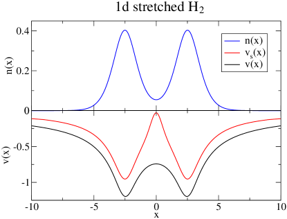
Figure 1: The KS potential for a stretched hydrogen molecule found from interacting electrons in 1d.

Our results are illustrated in Fig. 1, which shows 1d H₂ with soft-Coulomb interactions, plotted in atomic units. The exact density was found by DMRG and inverted to find the corresponding exact KS potential, $v_{\scriptscriptstyle\rm S}(x)$. The bond has been stretched beyond the Coulson–Fischer point, where Hartree–Fock and DFT approximations do poorly, as discussed further in Section IV.5. We comment here that a strong XC contribution to the KS potential is needed to reproduce the exact density in the bond region Helbig et al. (2009). Calculations to obtain the KS potential have often been performed for few-electron systems in 3d in the past Umrigar and Gonze (1994); Peirs et al. (2003), but our method allows exact treatment of systems with many electrons. In another paper Stoudenmire et al. , we show how powerful our DMRG method is, by solving a chain of 100 1d H atoms. All such calculations were previously unthinkable for systems of this size, and unreachable by any other method. We have applied these techniques to perform the first ever Kohn–Sham calculations using the exact XC functional, essentially implementing the exact Levy–Lieb constrained search definition of the functional, which we will present in yet another paper.

II Background in DMRG

The density matrix renormalization group (DMRG) is a powerful numerical method for computing essentially exact many-body ground-state wavefunctions White (1992, 1993). Traditionally, DMRG has been applied to 1d and quasi-2d finite-range lattice models for strongly correlated electrons Schollwöck (2005). DMRG has also been applied to systems in quantum chemistry, where the long-range Coulomb interaction is distinctive. The Hamiltonians which have been studied in this context include the Pariser–Parr–Pople model Fano et al. (1998) and the second-quantized form of the Hartree–Fock equations, where lattice sites represent electronic orbitals White and Martin (1999); Chan et al. (2008); Chan and Sharma (2011).

DMRG works by truncating the exponentially large basis of the full Hilbert space down to a much smaller one which is nevertheless able to represent the ground-state wavefunction accurately. Such a truncation would be highly inefficient in a real-space, momentum-space, or orbital basis; rather, the most efficient basis consists of the eigenstates of the reduced density matrix computed across bipartitions of the system White (1992). A DMRG calculation proceeds back and forth through a 1d system in a sweeping pattern, first optimizing the ground-state in the current basis then computing an improved basis for the next step. By increasing the number of basis states $m$ that are kept, DMRG can find the wavefunction to arbitrary accuracy.

The computational cost of DMRG scales as $N_{s}m^{3}$ where $N_{s}$ is the number of lattice sites. For gapped systems in 1d, the number of states $m$ required to compute the ground-state to a specified accuracy is independent of system size, allowing DMRG to scale linearly with $N_{s}$. For gapless or critical systems, the $m$ needed grows logarithmically with system size, making the scaling only slightly worse. The systems considered here have a relatively low total number of electrons such that the number of states $m$ required is small, often less than $100$. This in turn enables us to work with the very large numbers of sites ($N_{s}\sim 1000-5000$) needed to reach the continuum, as described in more detail below.

III Methodology

To apply DFT in its natural context—in the continuum—we shall consider a model of soft-Coulomb interacting matter Eberly et al. (1989); Thiele et al. (2008); Coe et al. (2011), where the electron repulsion has the form

$$v_{\rm ee}(u)=\dfrac{1}{\sqrt{u^{2}+1}},$$ (1)

and the interaction between an electron and a nucleus with charge $Z$ and location $X$ is

$$v(x)=-Zv_{\rm ee}(x-X).$$ (2)

The soft-Coulomb interaction is chosen to avoid divergences when particles are close to one another, and has been used to study molecules in intense laser fields Eberly et al. (1989); Thiele et al. (2008). The wavefunctions and densities within this model lack the cusps present in 3d Coulomb systems. However, the challenge presented by the long-range interactions in 3d Coulomb systems remains for these 1d model systems.

Although many methods could be used to solve these 1d systems, DMRG allows us to work efficiently with any arbitrary 1d real-space system, without the need to develop a basis for every 1d element. We enable DMRG to operate in the continuum by discretizing over a fine real-space grid. With a lattice spacing of $a$, the real-space Hamiltonian for a 1d system becomes in second quantized notation,

$$H =\sum_{j,\sigma}\frac{-1\ \ }{2a^{2}}(c^{\dagger}_{j\sigma}c_{j+1,\sigma}+c^{\dagger}_{j+1,\sigma}c_{j\sigma})-\tilde{\mu}\,n_{j\sigma}$$

$$\mbox{}+\sum_{j}v^{j}\,n_{j}+\frac{1}{2}\sum_{ij}v_{\rm ee}^{ij}\ n_{i}\,(n_{j}-\delta_{ij}),$$ (3)

where $\tilde{\mu}=\mu-1/a^{2}$, $v^{j}=v(j\,a)$ and $v_{\rm ee}^{ij}=v_{\rm ee}(|i-j|\,a)$. The $\delta_{ij}$ in the last term cancels self interactions. The operator $c^{\dagger}_{j\sigma}$ creates (and $c_{j\sigma}$ annihilates) an electron of spin $\sigma$ on site $j$, $n_{j}=n_{j\uparrow}+n_{j\downarrow}$, and $n_{j\sigma}=c^{\dagger}_{j\sigma}c_{j\sigma}$. The hopping terms $c^{\dagger}_{j\sigma}c_{j+1,\sigma}$ (and complex conjugate) come about from a finite-difference approximation to the second derivative. Like the second-quantized Hamiltonians considered in quantum chemistry, this Hamiltonian corresponds to an extended Hubbard model; Eq. (3), however, is motivated from a desire to study the 1d continuum alongside familiar DFT approximations. Because we require that the potentials and interactions vary slowly on the scale of the grid spacing, the low-energy eigenstates of the discrete Hamiltonian (3) will approximate the continuum system to very high accuracy. Moreover, we check convergence with respect to lattice spacing. Because our potentials—and thus our ground-state densities—vary slowly on the scale of the grid spacing, we can accelerate convergence by using a higher-order finite-difference approximation to the kinetic energy operator; this simply amounts to including more hopping terms in Eq. (3).

Even in its discretized form the Hamiltonian Eq. (3) represents a challenge for DMRG because of the long-range interactions. Including all $N_{s}\!^{2}$ interaction terms, where $N_{s}$ is the number of lattice sites, would make the calculation time scale as $N_{s}\!^{3}$ overall. Fortunately, an elegant solution has been recently developed Pirvu et al. (2010) which involves rewriting the Hamiltonian as a matrix product operator (MPO)—a string of operator-valued matrices. This form of the Hamiltonian is very convenient for DMRG, and MPOs naturally encode exponentially-decaying long-range interactions McCulloch (2007). Assuming that our interaction $v_{\rm ee}(u)$ can be approximated by a sum of exponentials, the the calculation time scales only linearly with the number of exponents $N_{\text{exp}}$ used. This reduces the computational cost from $N_{s}\!^{3}$ to $N_{s}\,N_{\text{exp}}$. In practice, for our soft-Coulomb interactions and modest system sizes ($N_{s}<1000$), we find that only $N_{\text{exp}}=20$ exponentials are needed to obtain an accuracy of $10^{-5}$ in our approximate $v_{\rm ee}(u)$. The largest $N_{\text{exp}}$ we use in this paper is $60$, which is necessary to find the equilibrium bond length of 1d H₂ accurate to $\pm 0.01$ bohr (a system with $N_{s}\approx 2000$).

For technical reasons, we take all of our systems to have open (or box) boundary conditions. This has no adverse effect on our results because we can extend the grid well past our edge atoms. The extra grid sites cost almost no extra simulation time due to the very low density of electrons in the edge regions. To evaluate the dependence of the energy on these edge effects and the grid size, consider Table 1. This table shows the convergence of the 1d model hydrogen atom ground-state energy with respect to the lattice spacing $a$ and the distance $c$ from the atom to the edge of the system, using the second-order finite difference approximation for the kinetic energy, as in Eq. (3). Our best estimate for the 1d H atom energy is -0.66977714, converged to at least microhartree accuracy, which differs slightly from that of Eberly et al., who were the first to consider the soft-Coulomb atom and its eigenstates Eberly et al. (1989).

$a$	$c=8$	$c=9$	$c=10$	$c\rightarrow\infty$
0.1000	-81.50	-82.30	-82.40	-82.41
0.0500	-19.58	-20.46	-20.57	-20.58
0.0200	-2.22	-3.16	-3.27	-3.29
0.0100	0.27	-0.68	-0.80	-0.82
0.0050	0.90	-0.07	-0.18	-0.20
0.0025	1.06	0.09	-0.03	-0.05
$\rightarrow 0$	1.12	0.14	0.02	0.00

Table 1: Convergence of model hydrogen energy with respect to lattice spacing $a$ and distance $c$ from the atom to the edge of the system, with differences in units of microhartree from the infinite continuum extrapolation of $E=-0.66977714$.

In addition to the accurate many-body solutions offered by DMRG, we can also look at approximate solutions given by standard quantum chemistry tools. Hartree–Fock (HF) theory can be formulated for these 1d systems by trivially changing out the Coulomb interaction for the soft-Coulomb. The exchange energy is then:

$$E_{\scriptscriptstyle\rm X} = -\frac{1}{2}\sum_{\sigma}\sum_{i,j=1}^{N_{\sigma}}\int dx\int dx^{\prime}\,v_{\rm ee}(x-x^{\prime})\times$$ (4)

$$\quad\quad\phi_{i\sigma}(x)\phi_{j\sigma}(x)\phi_{j\sigma}(x^{\prime})\phi_{i\sigma}(x^{\prime}).$$

In performing HF calculations, instead of using an orbital basis of Gaussians or some other set of functions, our “basis set” will be the grid, as in Eq. (3). This simple and brute force approach allows us a great degree of flexibility, but is only computationally tractable in 1d.

In this setting we also implement DFT. As mentioned in the introduction, DFT has been applied directly to lattice models. But our model and interaction are meant to mimic the usual application of DFT to the continuum. In particular, the LDA functionals we will use are similar to their 3d counterparts, unlike the Bethe ansatz LDA (BALDA), which has a gap built in Lima et al. (2003); Franca et al. . One calculates the LDA exchange energy by taking the exchange energy density per electron for a uniform gas of density $n$, namely $\epsilon^{\text{unif}}_{\scriptscriptstyle\rm X}(n)$, and then integrating it along with the electronic density:

$$E_{\scriptscriptstyle\rm X}^{\rm LDA}[n]=\int dx\,n(x)\,\epsilon^{\text{unif}}_{\scriptscriptstyle\rm X}\big{(}n(x)\big{)}.$$ (5)

We find $\epsilon^{\text{unif}}_{\scriptscriptstyle\rm X}(n)$ by evaluating Eq. (4) with the KS orbitals of a uniform gas. For a uniform gas, the KS orbitals are the eigenfunctions of a particle in a box, whose edges are pushed to infinity while the bulk density is kept fixed. Because the interaction has a length-scale, i.e. $v_{\rm ee}(\gamma u)\neq\gamma^{p}v_{\rm ee}(u)$ for some $p$, even exchange is not a simple function. One finds:

$$\epsilon_{\scriptscriptstyle\rm X}^{\rm unif}(n)=-n\,f(k_{\scriptscriptstyle\rm F})/2,$$ (6)

where $k_{\scriptscriptstyle\rm F}=\pi n/2$ is the Fermi wavevector and

$$f(z)=\int_{0}^{\infty}dy\,\frac{\sin^{2}y}{y^{2}}\frac{1}{{\sqrt{z^{2}+y^{2}}}}.$$ (7)

In fact, $f$ is related to the Meijer $G$ function:

$$f(z)=G^{2,2}_{2,4}\left(\begin{array}[]{c}\frac{1}{2},1\\ \frac{1}{2},\frac{1}{2},-\frac{1}{2},0\end{array}\Big{|}z^{2}\right)/(4z)\,.$$ (8)

We write $r_{s}=1/(2n)$ as the average spacing between electrons in 1d. In Fig. 2, we show the exchange energy per electron for the unpolarized gas as a function of $r_{s}$. For small $r_{s}$ (high density), $\epsilon_{\scriptscriptstyle\rm X}^{\text{unif}}\rightarrow-1/2+0.203\,r_{s}$; for large $r_{s}$ (low density), $\epsilon_{\scriptscriptstyle\rm X}^{\text{unif}}\rightarrow-0.291/r_{s}-\ln(r_{s})/(4r_{s})$. For contrast, in 3d, the exchange energy per electron is always $-0.458/r_{s}$ Dirac (1930), where $r_{s}=(3/(4\pi n))^{1/3}$.

In practice, we do not use pure DFT, but rather spin-DFT, in which all quantities are considered functionals of the up and down spin densities. In that case, we need LSD, the local spin-density approximation. For exchange, there is a simple spin scaling relation that tells us Fiolhais et al. (2003)

$$\epsilon_{\scriptscriptstyle\rm X}^{\rm unif}(n_{\uparrow},n_{\downarrow})=-n\,\sum_{\sigma=\pm 1}(1+\sigma\zeta)^{2}\,f(k_{\scriptscriptstyle\rm F}(1+\sigma\zeta))/4,$$ (9)

where $\zeta=(n_{\uparrow}-n_{\downarrow})/n$ is the polarization. This is less trivial than for simple Coulomb repulsion. At high densities, there is no increase in exchange energy due to spin polarization, while there is a huge increase (tending to a factor of 2) at low density, as shown by the solid black line in Fig. 2. In fact, $\epsilon_{\scriptscriptstyle\rm X}^{\rm unif}(r_{s},\zeta=1)=\epsilon_{\scriptscriptstyle\rm X}^{\rm unif}(r_{s}/2,\zeta=0)$.

To complete LDA, we need the correlation energy density of the uniform gas at various densities and polarizations. We are very fortunate to be able to make use of the pioneering work of Ref. Helbig et al. (2011), which performs just such a QMC calculation and parametrizes the results, yielding accurate values for $\epsilon_{\scriptscriptstyle\rm C}^{\text{unif}}(r_{s},\zeta)$, which are also plotted for the unpolarized and fully polarized cases in Fig. 2. These curves are not qualitatively similar to the 3d $\epsilon_{\scriptscriptstyle\rm XC}^{\text{unif}}(r_{s},\zeta)$. For these 1d model systems, the fully polarized electrons almost completely avoid one another at the exchange level, so that correlation barely decreases their energy for any value of $r_{s}$. For unpolarized electrons, the effect of correlation is to make them avoid each other entirely for low densities ($r_{s}>5$) and the XC energy per electron becomes independent of polarization. However, for unpolarized electrons at high density, correlation vanishes with $r_{s}$, and exchange dominates, as in the usual 3d case. For moderate $r_{s}$ values, the correlation contribution grows with $r_{s}$, as shown by the red dashed line of Fig. 2. To give an idea of what range of $r_{s}$ is important, for the hydrogen atom of Fig. 3, 95% of the density has $r_{s}(x)=(2\,n(x))^{-1}$ between 1 and 8.

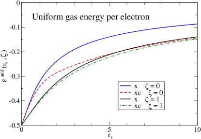
Figure 2: Parametrization of the LDA exchange and exchange-correlation energy densities per electron for polarized $\zeta=1$ and unpolarized $\zeta=0$ densities Helbig et al. (2011).

Armed with these parametrizations and tools, we are ready to discover 1d electronic structure.

IV Results

DMRG gives us an excellent tool for finding exact answers within a model 1d world. Our 1d world is designed to mimic qualitatively the 3d world, not match it exactly. Below we explain some important differences between our model 1d systems and real 3d systems, starting with the simplest element.

IV.1 One-electron atoms and ions

As we already mentioned, we find that the energy of the soft-Coulomb hydrogen atom is $E(H)=-0.66977714$, accurate to 1 microhartree. Its ground-state energy is similar to the 3d hydrogen atom energy of $-0.5$ a.u. Because the potential and wavefunction is much smoother, the kinetic energy is only 0.11 a.u., as opposed to 0.5 a.u. in 3d. Since the potential does not scale homogeneously, the virial theorem in 1d does not yield a simple relation among energy components, unlike in 3d.

Again because of the lack of simple scaling, hydrogenic energies do not scale quadratically for our system. A simple fit of energies for $Z\geq 1$ yields:

$$E_{Z}\approx-Z+\sqrt{Z}/2-{2}/{9}+{\alpha_{1}}/{\sqrt{Z}},~{}~{}~{}(N=1)$$ (10)

where $\alpha_{1}=0.0524$ is chosen to make the result accurate for $Z=1$. The first two coefficients are exact in the large-$Z$ limit, where the wavefunction is a Gaussian centered on the nucleus.

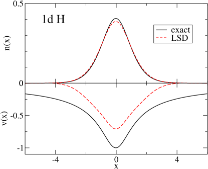
Figure 3: The hydrogen atom with both exact and LSD densities, as well as the LSD KS potential.

A well-known deficiency of approximate density functionals is their self-interaction error. Because $E_{\scriptscriptstyle\rm X}$ is approximated, usually in some local or semilocal form, it fails to cancel the Hartree energy for all one-electron systems. Thus, within LSD, the electron incorrectly repels itself. This error can be quantified by looking at how close $E_{\scriptscriptstyle\rm X}^{\rm LSD}$ is to the true $E_{\scriptscriptstyle\rm X}$. As can be seen in Table 2, $E_{\scriptscriptstyle\rm X}^{\rm LSD}$ is about 10% too small. For hydrogen, the self-interaction error is about 30 millihartrees. By adding in correlation, this error is slightly reduced, but remains finite. This is an example of the typical cancellation of errors between exchange and correlation in LSD.

system	$T$	$E$	​​$E^{\rm LSD}$	$E_{\scriptscriptstyle\rm X}$	$E^{\rm LSD}_{\scriptscriptstyle\rm X}$	$~{}E_{\scriptscriptstyle\rm C}^{\rm LSD}$
H	0.111	-0.670	-0.647	-0.346	-0.311	-0.007
He+	0.192	-1.483	-1.455	-0.380	-0.343	-0.006
Li++	0.258	-2.336	-2.304	-0.397	-0.359	-0.005
Be3+	0.316	-3.209	-3.176	-0.408	-0.369	-0.005

Table 2: Exact and LSD results for 1d one-electron systems.

As a result of self-interaction error, the LSD electron density spreads out too much, as shown in Fig. 3. In this figure we can also see how the LSD KS potential fails to replicate the true KS potential, which for hydrogen is the same as the external $v(x)$. And although the LSD KS potential is almost parallel to $v(x)$ where there is a large amount of density, it decays too rapidly as $|x|\to\infty$. What this adds up to, both in 1d and in 3d, is that LSD will not bind another electron easily, if at all. We will return to this point when considering anions.

IV.2 Two-electron atoms and ions

For two or more electrons, the HF approximation is not exact. The traditional quantum chemistry definition of correlation is the error made by HF:

$$E_{\scriptscriptstyle\rm C}^{\rm QC}=E-E^{\rm HF}.$$ (11)

In Table 3, we give accurate energy components for two-electron systems; recall that the components do not satisfy a virial theorem in our 1d systems. The total energy can be fit just as for one-electron systems, but now:

$$E_{Z}\approx-2\,Z+\sqrt{Z}+c_{0}-{\alpha_{2}}/{\sqrt{Z}},~{}~{}~{}(N=2)$$ (12)

where $c_{0}=0.507$ and $\alpha_{2}=0.235$. The HF energies may be fit with $c_{0}^{\rm HF}=0.476$ and $\alpha_{2}^{\rm HF}=0.167$. These fits are not accurate enough to give the large $Z$ behavior of $E_{\scriptscriptstyle\rm C}^{\rm QC}$, which seems to vanish as $Z\to\infty$. For 3d two-electron systems, the correlation energy scales to a constant at large $Z$ Frydel et al. (2000). Overall, $|E_{\scriptscriptstyle\rm C}^{\rm QC}|$ is much smaller in 1d than in 3d. Rather than the dimensionality, it is the soft nature of our Coulomb interactions that causes the reduction in correlation energy compared to 3d. The exact wavefunctions in 3d have cusps whenever two electrons of opposite spin come together, caused by the divergence of the electron-electron interaction. This cusp-related correlation is sometimes called dynamic correlation; any other correlation, involving larger separations of electrons, is called static Hollett and Gill (2011). (Note that the distinction between static and dynamic correlation is not precise.) Our soft-Coulomb potential has no divergence and induces no cusps, so dynamical correlation is minimal. There is little static correlation in tightly bound closed shell systems, such as our 1d Li⁺ and Be⁺⁺, so $|E_{\scriptscriptstyle\rm C}^{\rm QC}|\ll|E|$. In contrast, for H^-, where one electron is loosely bound, one expects most of the correlation to be static even in 3d, and one sees large and similar $E_{\scriptscriptstyle\rm C}$ values in 1d and 3d. In Section IV.5, we discuss some quantitative measures of strong correlation.

system	$T$	$V$	$V_{\rm ee}$	$E$	$E^{\rm HF}$	$E_{\scriptscriptstyle\rm C}^{\rm QC}$
H-	0.115	-1.326	0.481	-0.731	-0.692	-0.039
He	0.290	-3.219	0.691	-2.238	-2.224	-0.014
Li+	0.433	-5.084	0.755	-3.896	-3.888	-0.008
Be++	0.556	-6.961	0.790	-5.615	-5.609	-0.006
3d H-	0.528	-1.367	0.311	-0.528	-0.488	-0.042
3d He	2.904	-6.753	0.946	-2.904	-2.862	-0.042
3d Li+	7.280	-16.13	1.573	-7.280	-7.236	-0.043
3d Be++	13.66	-29.50	2.191	-13.66	-13.61	-0.044

Table 3: Exact and HF two-electron atoms and ions, in 1- and 3-d (exact data from Ref. Umrigar and Gonze (1994), Li⁺ is fit quadratically to surrounding elements, and HF data from Refs. III (2011); Davidson et al. (1991)).

Next we study the exact Kohn–Sham DFT energy components of these two-electron systems. Here we need the DFT definition of correlation, which differs slightly from the traditional quantum chemistry version:

$$E_{\scriptscriptstyle\rm C} = E-(T_{\scriptscriptstyle\rm S}+V+U+E_{\scriptscriptstyle\rm X})$$ (13)

$$= T_{\scriptscriptstyle\rm C}+U_{\scriptscriptstyle\rm C},$$

where $E_{\scriptscriptstyle\rm X}$ is the exchange energy of the exact KS orbitals, $T_{\scriptscriptstyle\rm S}$ is their kinetic energy, $U$ is the Hartree energy, $T_{\scriptscriptstyle\rm C}=T-T_{\scriptscriptstyle\rm S}$ is the kinetic correlation energy, and $U_{\scriptscriptstyle\rm C}=V_{\rm ee}-U-E_{\scriptscriptstyle\rm X}$ is the potential correlation energy. All these functionals are evaluated on the exact ground-state density, with numerical results found in Table 4. The difference between the quantum chemistry $E_{\scriptscriptstyle\rm C}^{\rm QC}$ and the DFT $E_{\scriptscriptstyle\rm C}$ is never negative and typically much smaller than $|E_{\scriptscriptstyle\rm C}|$ Gross et al. (1996). For the two-electron systems of Table 3 and Table 4, the difference is zero to the given accuracy for all atoms and ions besides 1d H^-. For our systems, just as in 3d, $E_{\scriptscriptstyle\rm C}^{\rm QC}-E_{\scriptscriptstyle\rm C}$ vanishes as $Z\to\infty$. All the large DFT components ($T_{\scriptscriptstyle\rm S}$, $U$, $E_{\scriptscriptstyle\rm XC}$) are typically smaller than their 3d counterparts and scale much more weakly with $Z$. However, our numerical results suggest $T_{\scriptscriptstyle\rm C}\to-E_{\scriptscriptstyle\rm C}$ as $Z\to\infty$, just as in 3d.

system	$T_{\scriptscriptstyle\rm S}$	$U$	$E_{\scriptscriptstyle\rm XC}$	$E_{\scriptscriptstyle\rm X}$	$E_{\scriptscriptstyle\rm C}$	$T_{\scriptscriptstyle\rm C}$
H-	0.087	1.103	-0.595	-0.552	-0.043	0.028
He	0.277	1.436	-0.733	-0.718	-0.014	0.013
Li+	0.425	1.542	-0.779	-0.771	-0.008	0.008
Be++	0.551	1.601	-0.806	-0.801	-0.006	0.005
3d H-	0.500	0.762	-0.423	-0.381	-0.042	0.028
3d He	2.867	2.049	-1.067	-1.025	-0.042	0.037
3d Li+	7.238	3.313	-1.699	-1.656	-0.043	0.041
3d Be++	13.61	4.553	-2.321	-2.277	-0.044	0.041

Table 4: Energies of the exact KS system for two-electron atoms and ions. 3d data (Li⁺ fitted) from Ref. Umrigar and Gonze (1994).

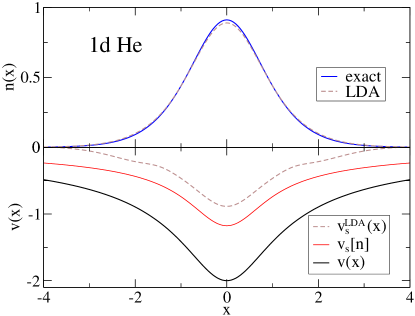
Figure 4: The exact KS potential for a model helium density found from interacting electrons in 1d, as well as the LDA density and LDA KS potential found self-consistently.

To obtain the KS energies for a given problem, we require the KS potential, which is found by inverting the KS equation. For one- or two-electron systems, this yields:

$$v_{\scriptscriptstyle\rm S}(x)=\dfrac{1}{2\sqrt{n(x)}}\dfrac{d^{2}}{dx^{2}}\sqrt{n(x)}.\quad{(N\leq 2)}$$ (14)

For illustration, consider the exact KS potential of 1d helium in Fig. 4. Inverting a density to find the KS potential has also been done for small systems in 3d, where QMC results for a correlated electron density have proven extremely useful Umrigar and Gonze (1994). One can find simple and useful constraints on the KS potential by studying the large and small $r$ behavior of the exact result Umrigar and Gonze (1994); Levy et al. (1984). In 3d, for large $r$, the Hartree potential screens the nuclear potential, and the exchange-correlation potential goes like $-1/r$ Almbladh and Pedroza (1984). In 1d, the softness of the Coulomb potential is irrelevant, so the Hartree potential screens the nuclear potential for large $|x|$ as in 3d. Though it seems likely, we have no proof that the exchange-correlation potential for the soft-Coulomb interaction should tend to $-1/|x|$ for large $|x|$, analogous to the 3d Coulomb result. To check this would require extreme numerical precision in the density far from the atom, due to the need to evaluate Eq. (14) where the density is exponentially small. Instead, in Figures 1 and 4, we require the KS potential to go as $-b/|x|$ once the density becomes too small (around $n\approx 10^{-5}$, which happens at $|x|\approx 6$ for helium), and we choose $b$ to enforce Koopmans’ theorem for KS-DFT. The actual value of $b$ has no visible effect on the density on the scale of these figures.

We now consider the performance of LDA for these two-electron systems, starting with how well LDA replicates the true KS potential. Though the LDA density is only slightly different from the exact density on the scale of Fig. 4, the LDA potential clearly decays too rapidly (exponentially) at large $r$ and is too shallow overall, just as in 3d Umrigar and Gonze (1994). Like the hydrogen atom discussed earlier, this is a result of self-interaction error. LDA energy results are given in Table 5. Clearly LDA becomes relatively more accurate as $Z$ grows, because XC becomes an ever smaller fraction of the total energy. Comparing Tables 4 and 5, we also see that LDA underestimates the true X contribution by about 10%, while overestimating the correlation contribution, so that XC itself has lower error than either, i.e., a cancellation of errors.

system	$E^{\rm LDA}$	% error	$E_{\scriptscriptstyle\rm XC}^{\rm LDA}$	$E_{\scriptscriptstyle\rm X}^{\rm LDA}$	$E_{\scriptscriptstyle\rm C}^{\rm LDA}$
H-	-0.708	-3.1%	-0.601	-0.536	-0.065
He	-2.201	-1.7%	-0.690	-0.646	-0.044
Li+	-3.850	-1.2%	-0.731	-0.696	-0.035
Be++	-5.564	-0.9%	-0.753	-0.723	-0.030
3d H-	-0.511	-3.2%	-0.419	-0.345	-0.074
3d He	-2.835	-2.4%	-0.973	-0.862	-0.111
3d Li+	-7.143	-1.9%	-1.531	-1.396	-0.134
3d Be++	-13.44	-1.2%	-2.082	-1.931	-0.150

Table 5: LDA for 2 electron systems. H^- does not converge in 1d or 3d; the results are taken from using the LDA functional on the HF density Lee and Burke (2010). 3d LDA data from Engel’s OEP code Engel and Dreizler (1999).

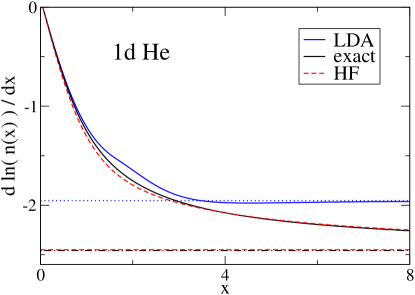
Figure 5: The differential logarithmic decay of the helium atom density for various methods. The horizontal, dashed lines correspond to the asymptotic decay constants.

Much insight into density functionals has been gained by studying the asymptotic decay of densities and potentials far from the nucleus Levy et al. (1984). In Fig. 5, we plot $dn/dx/n$ to emphasize the asymptotic decay of the exact, LDA, and HF helium densities. The HF density is very accurate compared to the LDA density. For large $x$, the HF density has very nearly the same behavior as the exact density, and both approach their asymptotes very slowly. By contrast, the LDA density reaches its asymptote by $x\approx 4$. For each approximate calculation, its asymptotic decay constant $\gamma$ can be found using the highest occupied molecular orbital (HOMO) energy: $\gamma=-2\sqrt{-2\epsilon_{\text{HOMO}}}$. The asymptote for the exact curve can be found using the ionization potential $I=E(N-1)-E(N)$ of the system, which determines the density decay: $\gamma=-2\sqrt{2I}$. Because the HF asymptote lies nearly on top of the exact asymptote, Koopmans’ theorem—or $I\cong-\epsilon_{\text{HOMO}}^{\text{HF}}$—is extremely accurate for 1d helium. We list both HOMO and total energy differences in Table 6.

	LSD		HF		exact
system	-$\epsilon_{\text{HOMO}}$	$I$	-$\epsilon_{\text{HOMO}}$	$I$	$I=$-$\epsilon_{\text{HOMO}}$
H-	—	0.062	0.054	0.022	0.061
He	0.478	0.747	0.750	0.741	0.755
Li+	1.242	1.546	1.557	1.552	1.560
Be++	2.064	2.389	2.404	2.400	2.406

Table 6: 1d HOMO eigenvalues and ionization potentials of two-electron atoms and ions, for the exact functional, LDA, and HF. LDA does not converge for H^- anion, but LDA energies can be found using the HF density Lee and Burke (2010).

There is a long history of studying two-electron ions in DFT, including the smallest anion H^-, which presents interesting conundrums for approximate functionals Shore et al. (1977); Kim et al. (2011). Looking at the ionization energies of these 2 electron systems, we can extrapolate the critical nuclear charge necessary for binding two electrons, i.e., figuring out the $Z$ value for which $I=0$. This happens around $Z=0.90$ in 1d, and around $Z=0.91$ in 3d Bransden and Joachain (2003). Within LDA, the critical value is above $Z=1$, because H^- will not bind. DFT approximations have a hard time binding anions—both in 1d and in 3d—due to self-interaction error. A way to circumvent this problem is to take the HF anion, which binds an extra electron, and evaluate the LDA functional on its density. As seen in Table 6, this approach is far better than either taking total energy differences or the negative of the HOMO energy from HF alone, just as in 3d Lee and Burke (2010). As in 3d, $-\epsilon_{\text{HOMO}}^{\rm LSD}$ is useless as an approximation to $I$. The HF results $-\epsilon_{\text{HOMO}}^{\rm HF}$ and $I^{\rm HF}$ are close to each other and closest to $I$ for larger $Z$; but $I^{\rm LSD}$ does very well for small $Z$, and is best for H^-.

IV.3 Many-electron atoms

Before looking at larger atoms, a word of caution. In 3d systems, degeneracies in orbitals with different angular momentum quantum numbers produce interesting shell structure. In 1d, there is no angular momentum—each 1d shell is either half-filled or filled—so it is not clear which real elements our model 1d atoms correspond to. The first three 1d elements might well be called hydrogen, helium, and lithium; but the fourth 1d element may behave more like neon than beryllium. To be consistent with Ref. Helbig et al. (2011), we call it beryllium. To showcase 1d Be, consider its LDA treatment in Fig. 6. The exact KS potential is also plotted, and the LDA KS potential roughly differs only by a constant in the high density region, just as with hydrogen (Fig. 3) and helium (Fig. 4). In the low density regions, the LDA correlation potential is the dominant piece of the LDA KS potential.

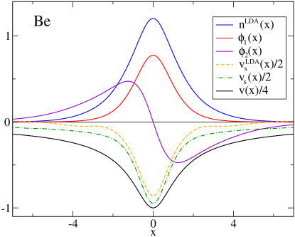
Figure 6: An LDA “beryllium” atom, complete with the LDA orbitals $\phi_{j}(x)$, LDA KS potential $v_{\scriptscriptstyle\rm S}^{\rm LDA}(x)$, exact KS potential $v_{\scriptscriptstyle\rm S}(x)$, and external potential $v(x)$. The density $n^{\rm LDA}(x)$ was found self-consistently using the LDA method, and barely differs from the true $n(x)$ on this scale.

As we increase the number $N$ of electrons in our systems, correlation also increases, but HF theory is still better than LDA until $N=4$. Exact and HF data for many-electron atoms can be found in Table 7, and LDA data in Table 8. Despite good agreement with all other data, we did not find He^- or Li^- to bind as in Ref. Helbig et al. (2011), neither in HF nor DMRG, nor LSD (not surprisingly). When using energy differences to calculate the ionization energy, HF outperforms LSD until beryllium, as can be seen in Table 9. For these systems, $I^{\rm LSD}>I>I^{\rm HF}$: LSD overestimates the ionization energy, and HF underestimates it—just as in 3d. As with the fewer electron systems, the LSD HOMO energies are not a good way to estimate $I$, whereas the HF HOMO energies are.

system	$T$	$V$	$V_{\rm ee}$	$E$	$E^{\rm HF}$	$E_{\scriptscriptstyle\rm C}^{\rm QC}$
Li	0.625	-6.484	1.648	-4.211	-4.196	-0.015
Be+	0.922	-9.240	1.864	-6.454	-6.445	-0.010
Be	1.127	-11.13	3.219	-6.785	-6.740	-0.046

Table 7: Exact and HF many-electron atoms and ions, in 1d.

	$E^{\rm LSD}$	% error	$E_{\scriptscriptstyle\rm XC}^{\rm LSD}$	$E_{\scriptscriptstyle\rm X}^{\rm LSD}$	$E_{\scriptscriptstyle\rm C}^{\rm LSD}$
Li	-4.179	-0.8%	-1.044	-1.004	-0.041
Be+	-6.410	-0.7%	-1.117	-1.086	-0.031
Be	-6.764	-0.3%	-1.450	-1.376	-0.075

Table 8: LSD energies for many-electron 1d systems.

	LSD		HF		exact
system	-$\epsilon_{\text{HOMO}}$	$I$	-$\epsilon_{\text{HOMO}}$	$I$	$I=$-$\epsilon_{\text{HOMO}}$
Li	0.166	0.329	0.316	0.308	0.315
Be+	0.628	0.846	0.842	0.835	0.839
Be	0.162	0.353	0.313	0.295	0.331

Table 9: Many-electron ionization energies for LSD, HF, and exact 1d systems.

To find the KS energy components for these many-electron ($N>2$) systems, we again require the exact KS potential. For these systems, Eq. (14) is no longer valid, so we must find the KS potential another way. The simplest procedure is to use guess-and-check, adjusting the KS potential until its density can no longer be distinguished from the target density found using DMRG. Updates to the KS potential can be more or less sophisticated without changing the final result in the region where the density is large; in the low-density region, however, two very different KS potentials can give rise to densities that are indistinguishable on the scale of our figures. However, the KS energy components do not rely significantly on the behavior of the KS potential out in the low-density region. In Table 10, the exact KS energies for some many-electron systems are tabulated. For Li and Be⁺, spin-DFT is used, but the spin-dependent energy components (such as $T_{\scriptscriptstyle\rm S}^{\sigma}$) are summed together to give a spin-independent energy.

	$T_{\scriptscriptstyle\rm S}$	$U$	$E_{\scriptscriptstyle\rm XC}$	$E_{\scriptscriptstyle\rm X}$	$E_{\scriptscriptstyle\rm C}$	$T_{\scriptscriptstyle\rm C}$
Li	0.611	2.749	-1.087	-1.071	-0.016	0.014
Be+	0.912	3.042	-1.168	-1.157	-0.011	0.009
Be	1.091	4.736	-1.481	-1.430	-0.051	0.036

Table 10: Energies of the exact KS system for many-electron 1d atoms and ions.

The study of the energies of neutral atoms as $N=Z\to\infty$ is important due to the semiclassical result being exact in that limit Elliott et al. (2008). In this limit, the oldest of all density functional approximations, Thomas–Fermi (TF) theory, becomes exact Lieb (1981). However, due to a lack of scaling within the soft-Coulomb interaction, the large $Z$ limit of the energy is non-trivial, making a semiclassical treatment difficult. A plot of the neutral atom energies as a function of $N$ appears in Fig. 7. On this scale, both the LDA and HF results lie nearly on top of the exact curve.

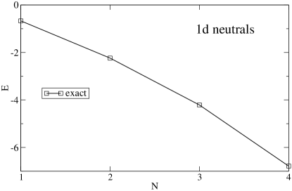
Figure 7: Energies of neutral atoms in 1d.

IV.4 Equilibrium properties of small molecules

We now briefly discuss small molecules near their equilibrium separation. In order to find the equilibrium bond length for our 1d systems, we take the nuclei to be interacting via the soft-Coulomb interaction, just like the electrons. Given this interaction, consider the simplest of all molecules: the H${}_{2}^{+}$ cation. HF yields the exact answer, and LSD suffers from self-interaction (more generally, a delocalization error Cohen et al. (2008)). A plot of the binding energy is found in Fig. 8. Because the nuclear-nuclear repulsion is softened, the binding energy does not diverge as the internuclear separation $R$ goes to zero. As seen in Table 11, LSD overbinds slightly and produces bonds that are too long between H atoms, which is also the case in 3d. The curvature of the LSD binding energy is too small near equilibrium, which makes for inaccurate vibrational energies, especially in 3d. This can also be seen in Table 11. Finally, we note that the energy of stretched H${}_{2}^{+}$ does not tend to that of H within LSD, due to delocalization error Cohen et al. (2008).

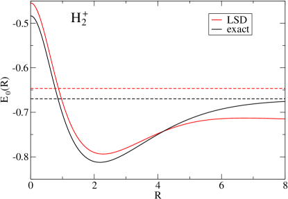
Figure 8: The binding energy curve for our 1d model H${}_{2}^{+}$, shown with an absolute energy scale, and with nuclear separation $R$; horizontal dashed lines indicate the energy of a single H atom.

	HF	LSD	exact
system	$D_{\text{e}}$ (eV)
H${}_{2}^{+}$	3.88  (0%)	4.00  (3%)	3.88
3d H${}_{2}^{+}$	2.77  (0%)	2.89  (4%)	2.77
H2	2.36 (-23%)	3.53 (15%)	3.07
3d H2	3.54 (-25%)	4.80  (1%)	4.75
system	$R_{0}$
H${}_{2}^{+}$	2.18  (0%)	2.28  (4%)	2.18
3d H${}_{2}^{+}$	2.00  (0%)	2.18  (9%)	2.00
H2	1.50  (-6%)	1.63  (2%)	1.60
3d H2	1.41  (1%)	1.47  (5%)	1.40
system	$\omega$ ($\times 10^{3}$ cm-1)
H${}_{2}^{+}$	2.2  (0%)	2.0  (-9%)	2.2
3d H${}_{2}^{+}$	2.4  (0%)	1.9 (-21%)	2.4
H2	3.3  (6%)	3.0  (-3%)	3.1
3d H2	4.6  (5%)	4.2  (-5%)	4.4

Table 11: Electronic well depth $D_{\text{e}}$, equilibrium bond radius $R_{0}$, and vibrational frequency $\omega$ for the H${}_{2}^{+}$ and H₂ molecules, with percentage error in parentheses. Exact 3d H₂ results taken from Ref. Kolos and Wolniewicz (1968); the remaining 3d values are from Ref. III (2011) using the aug-cc-pVDZ basis set Weigend et al. (2002).

Next we consider H₂. A plot of the binding energy is found in Fig. 9; the large $R$ behavior will be discussed in the following section. Just as in 3d, HF underbinds while LDA overbinds; HF bonds are too short, and LDA bonds are too long. Further, HF yields vibrational frequencies which are too high, and LDA are a little small, which is the case both in 1d and 3d. All of these properties can be seen in Table 11.

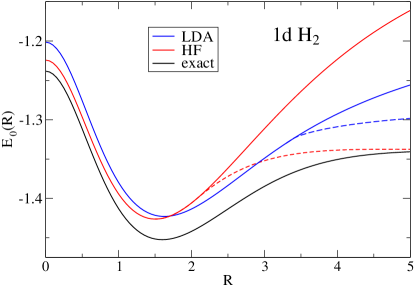
Figure 9: The binding energy curve for our 1d model H₂, shown on an absolute energy scale, with nuclear separation $R$. Dashed curves represent unrestricted calculations.

IV.5 Quantifying correlation

It is often said that DFT works well for weakly correlated systems, but fails when correlation is too strong. Strong static correlation, which occurs when molecules are pulled apart, is also identified with strong correlation in solids Cohen et al. (2008). Functionals that can accurately deal with strong static correlation in stretched molecules can also accurately yield the band gap of a solid Mori-Sánchez et al. (2008); Zheng et al. (2011). Most DFT methods, however, fail in these situations. To see these effects in 1d, we shall now examine three descriptors of strong correlation, which will be 0 when no correlation is present and close to 1 when strong correlation is present.

A simple descriptor of strong correlation is simply to calculate the ratio of correlation to exchange:

$$\alpha=\dfrac{E_{\scriptscriptstyle\rm C}}{E_{\scriptscriptstyle\rm X}}.$$ (15)

In the limit of weak electron-electron repulsion, $\alpha$ goes to zero for closed-shell systems, and HF becomes exact. For example, for the two-electron atoms and ions in Table 4, $\alpha$ goes to zero as $Z$ increases. In Table 12, we compute $\alpha$ for various bond lengths of the hydrogen molecule, both in 1d and in 3d. At the equilibrium bond length, $\alpha$ is small, indicating that the HF solution is very close to the exact. When the bond is stretched to $R=5$, $\alpha$ increases ten-fold: a standard HF solution for a bond length of $R=5$ does not do well at all. The 1d and 3d results are remarkably similar. We can also compute $\alpha$ using the LDA functionals for $E_{\scriptscriptstyle\rm C}$ and $E_{\scriptscriptstyle\rm X}$ evaluated on the LDA density; however, $\alpha^{\rm LDA}$ is not as good of an indicator for strong correlation as the true $\alpha$ is.

The second descriptor of strong correlation requires first understanding where correlation comes from. From Eq. (13), correlation can be separated into two pieces: (1) the kinetic correlation energy $T_{\scriptscriptstyle\rm C}=T-T_{\scriptscriptstyle\rm S}$, due to the small difference between the true kinetic energy and the KS kinetic energy, and (2) potential correlation energy, $U_{\scriptscriptstyle\rm C}=V_{\rm ee}-U-E_{\scriptscriptstyle\rm X}$. In the limit of weak correlation in 3d, $U_{\scriptscriptstyle\rm C}\rightarrow-2T_{\scriptscriptstyle\rm C}$, so the ratio:

$$\beta=\frac{E_{\scriptscriptstyle\rm C}+T_{\scriptscriptstyle\rm C}}{E_{\scriptscriptstyle\rm C}}$$ (16)

has always been found to be positive, and vanishes in the weakly correlated limit Burke et al. (1997), which we have also observed in 1d. But if $T_{\scriptscriptstyle\rm C}\ll|E_{\scriptscriptstyle\rm C}|$, we have correlation without the usual kinetic contribution, which occurs when systems have strong static correlation. For example, in the infinitely stretched limit of H₂, $T_{\scriptscriptstyle\rm S}\to T$ while $E_{\scriptscriptstyle\rm C}$ remains finite, so $\beta\to 1$. In Table 12, we see that $\beta$ increases as we stretch the H₂ molecule, both in 1d and 3d. Thus $\beta$ is a natural measure of static correlation in chemistry.

There is another test for strong static correlation, which we can use on closed-shell systems: whether an approximate calculation prefers to break spin-symmetry or not. This well-known phenomenon occurs when a molecule, such as H₂, is stretched beyond the Coulson–Fischer point Coulson and Fischer (1949), and indicates the preference for electrons to localize on different atoms. Spin-symmetry-breaking can be observed in Fig. 9, where the solid (dashed) curves represent restricted (unrestricted) calculations for a stretched hydrogen molecule. Unrestricted HF/LSD breaks spin symmetry around $R=2.1$/3.4, beyond which the unrestricted solution gives accurate total energies, but very incorrect spin densities Perdew et al. (1995). The numbers are similar in 3d ($R=2.3$/3.3) Bauernschmitt and Ahlrichs (1996).

		1d			3d
	$R$	1.6	3.4	5.0	1.4	5.0
exact	$\alpha$	0.04	0.21	0.46	0.06	0.45
	$\beta$	0.21	0.58	0.87	0.18	0.89
LDA	$\alpha$	0.09	0.16	0.21

Table 12: Table of correlation descriptors $\alpha$ and $\beta$ (Eqs. (15) and (16)) for H₂ at an equilibrium and a stretched bond length $R$. 3d data from Ref. Fuchs et al. (2005).

V Conclusion

In this paper, we have surveyed basic features of the electronic structure of a one-dimensional world of electrons and protons interacting via a soft-Coulomb interaction. We have established many key reference values for future use in calculations of atoms, molecules, and even solids. This 1d world forms a virtual laboratory for understanding and improving electronic structure methods. A major advantage of the 1d world is provided by DMRG which is extremely efficient and accurate for such systems, making large system sizes readily accessible. Furthermore, the thermodynamic limit is far more quickly approached in 1d than in 3d.

But none of this would be useful if, in this 1d world, both exact and approximate calculations did not behave qualitatively similarly to their 3d analogs. If bonds are not formed or ions do not exist, there would be no 1d analog of many of the energy differences that are used as real electronic stucture benchmarks. This work contains an extremely detailed study of the qualitative similarities, and differences, between this 1d world and our own.

For atoms and cations, we find trends in the exact numbers quite similar to real atoms. However, densities are more diffuse and correlation is weaker, so that Hartree-Fock is more accurate than in 3d. An important technical difference is that the interaction does not scale simply under coordinate scaling, so that even hydrogenic atoms do not scale simply with $Z$, and there is no simple virial relation among the energy components of atoms and ions. Perhaps the most important caveat is that, while atoms with more than 2 electrons exist, there are no orbital shells in 1d, so there is no clear analog to specific real atoms. Our 1d periodic table has only two columns.

Equally important, if the 1d world is to be useful in studying DFT, is that the standard approximations work and fail under the same circumstances as in 3d. We have shown that spin-polarization effects can be much stronger in the 1d uniform gas than in 3d, and this has an effect on the local (spin) density approximation. But LSD behaves very similarly to its 3d analog, not just for energetics, but also in the poor behavior of the potential and HOMO eigenvalue.

For the prototype molecules, H₂ and H${}_{2}^{+}$, we find LDA working well at equilibrium, with errors similar to those in 3d. As the bonds are stretched and correlation effects grow, H${}_{2}^{+}$ shows the usual self-interaction or delocalization error, while approximate treatments of H₂ break symmetry, just as in 3d. Remarkably, simple measures of correlation at both equilibrium and stretched bonds are quantitatively similar to their 3d counterparts.

These results suggest that understanding electron correlation in this 1d world will provide insight into real 3d systems, and illuminate the challenges to making approximate DFT work for strongly correlated systems. Other approximate approaches to correlation, such as range-separated hybrids Savin (1996), dynamical mean-field theory Georges et al. (1996), and LDA+U Anisimov et al. (1997), can be tested in the future. Furthermore, fragmentation schemes such as partition density functional theory (PDFT) Elliott et al. (2010), can be tested for fully interacting fragments using the exact exchange-correlation functional, calculated via DMRG. We expect many further 1d explorations in the future.

With gratefulness, we acknowledge DOE grant DE-FG02-08ER46496 (KB and LW) and NSF grant DMR-0907500 (ES and SW) for supporting this work.

References

- Kohn and Sham (1965) W. Kohn and L. J. Sham, “Self-consistent equations including exchange and correlation effects,” Phys. Rev. 140, A1133–A1138 (1965).
- Ceder et al. (1998) G. Ceder, Y. M. Chiang, D. R. Sadoway, M. K. Aydinol, Y. I. Jang, and B. Huang, “Identification of cathode materials for lithium batteries guided by first-principles calculations,” Nature 392, 694–696 (1998).
- Hammer and Norskov (2000) B Hammer and JK Norskov, “Theoretical surface science and catalysis - Calculations and concepts,” in Advances in catalysis, Vol 45: Impact of surface science on catalysis, Advances in Catalysis, Vol. 45, edited by Gates, BC and Knozinger, H (2000) pp. 71–129.
- Casely et al. (2011) I. J. Casely, J. W. Ziller, M. Fang, F. Furche, and W. J. Evans, “Facile bismuth-oxygen bond cleavage, c-h activation, and formation of a monodentate carbon-bound oxyaryl dianion, (c6hbu2-3,5-o-4)2-,” J. Am. Chem. Soc. 133, 5244–5247 (2011).
- Cohen et al. (2008) Aron J. Cohen, Paula Mori-Sanchez, and Weitao Yang, “Insights into current limitations of density functional theory,” Science 321, 792–794 (2008).
- Mori-Sánchez et al. (2009) Paula Mori-Sánchez, Aron J. Cohen, and Weitao Yang, “Discontinuous nature of the exchange-correlation functional in strongly correlated systems,” Phys. Rev. Lett. 102, 066403 (2009).
- Heyd et al. (2003) Jochen Heyd, Gustavo E. Scuseria, and Matthias Ernzerhof, “Hybrid functionals based on a screened coulomb potential,” The Journal of Chemical Physics 118, 8207–8215 (2003), ibid. 124, 219906(E) (2006).
- Georges et al. (1996) Antoine Georges, Gabriel Kotliar, Werner Krauth, and Marcelo J. Rozenberg, “Dynamical mean-field theory of strongly correlated fermion systems and the limit of infinite dimensions,” Rev. Mod. Phys. 68, 13–125 (1996).
- Jensen (2006) Frank Jensen, Introduction to Computational Chemistry (Wiley, 2006).
- Umrigar and Nightingale (1999) Cyrus J. Umrigar and M.P. Nightingale, Quantum Monte Carlo Methods in Physics and Chemistry, Vol. 525 (Springer, 1999).
- Martin (2004) Richard Martin, Electronic Structure (Cambridge University Press, Cambridge, 2004).
- White (1992) Steven R. White, “Density matrix formulation for quantum renormalization groups,” Phys. Rev. Lett. 69, 2863 (1992).
- White (1993) Steven R. White, “Density-matrix algorithms for quantum renormalization groups,” Phys. Rev. B 48, 10345 (1993).
- Schollwöck (2005) U. Schollwöck, “The density-matrix renormalization group,” Rev. Mod. Phys. 77, 259–315 (2005).
- Chan and Sharma (2011) Garnet Kin-Lic Chan and Sandeep Sharma, “The density matrix renormalization group in quantum chemistry,” Annual Review of Physical Chemistry 62, 465–481 (2011).
- Hubbard (1963) J. Hubbard, “Electron correlations in narrow energy bands,” Proceedings of the Royal Society of London. Series A, Mathematical and Physical Sciences 276 (1963).
- (17) E.M. Stoudenmire, Lucas O. Wagner, Steven R. White, and Kieron Burke, “One-dimensional continuum electronic structure calculations with the density matrix renormalization group,” arXiv:1107.2394v1 .
- Helbig et al. (2011) N. Helbig, J. I. Fuks, M. Casula, M. J. Verstraete, M. A. L. Marques, I. V. Tokatly, and A. Rubio, “Density functional theory beyond the linear regime: Validating an adiabatic local density approximation,” Phys. Rev. A 83, 032503 (2011).
- Helbig et al. (2009) N. Helbig, I. V. Tokatly, and A. Rubio, “Exact kohn–sham potential of strongly correlated finite systems,” J. Chem. Phys. 131, 224105 (2009).
- Umrigar and Gonze (1994) C. J. Umrigar and Xavier Gonze, “Accurate exchange-correlation potentials and total-energy components for the helium isoelectronic series,” Phys. Rev. A 50, 3827–3837 (1994).
- Peirs et al. (2003) K. Peirs, D. Van Neck, and M. Waroquier, “Algorithm to derive exact exchange-correlation potentials from correlated densities in atoms,” Phys. Rev. A 67, 012505 (2003).
- Fano et al. (1998) G. Fano, F. Ortolani, and L. Ziosi, “The density matrix renormalization group method: Application to the PPP model of a cyclic polyene chain,” The Journal of Chemical Physics 108, 9246–9252 (1998).
- White and Martin (1999) Steven R. White and Richard L. Martin, “Ab initio quantum chemistry using the density matrix renormalization group,” J. Chem. Phys. 110, 4127 (1999).
- Chan et al. (2008) G. K-L. Chan, J. J. Dorando, D. Ghosh, J. Hachmann, E. Neuscamman, H. Wang, and T. Yanai, “An introduction to the density matrix renormalization group ansatz in quantum chemistry,” Prog. Theor. Chem. and Phys. 18, 49 (2008).
- Eberly et al. (1989) J. H. Eberly, Q. Su, and J. Javanainen, “High-order harmonic production in multiphoton ionization,” J. Opt. Soc. Am. B 6, 1289–1298 (1989).
- Thiele et al. (2008) M. Thiele, E. K. U. Gross, and S. Kümmel, “Adiabatic approximation in nonperturbative time-dependent density-functional theory,” Phys. Rev. Lett. 100, 153004 (2008).
- Coe et al. (2011) J. P. Coe, V. V. Franca, and I. D’Amico, “Feasibility of approximating spatial and local entanglement in long-range interacting systems using the extended hubbard model,” EPL (Europhysics Letters) 93, 10001 (2011).
- Pirvu et al. (2010) B. Pirvu, V. Murg, J. I. Cirac, and F. Verstraete, “Matrix product operator representations,” New J. Phys. 12, 025012 (2010).
- McCulloch (2007) Ian P. McCulloch, “From density-matrix renormalization group to matrix product states,” J. Stat. Mech. , P10014 (2007).
- Lima et al. (2003) N. A. Lima, M. F. Silva, L. N. Oliveira, and K. Capelle, “Density functionals not based on the electron gas: Local-density approximation for a luttinger liquid,” Phys. Rev. Lett. 90, 146402 (2003).
- (31) Vivian V. Franca, Daniel Vieira, and Klaus Capelle, “Analytical parametrization for the ground-state energy of the one-dimensional hubbard model,” arXiv:1102.5018v1 .
- Note (1) Information about the Meijer function can be found online at http://mathworld.wolfram.com/MeijerG-Function.html.
- Dirac (1930) P. A. M. Dirac, “Note on exchange phenomena in the Thomas atom,” Mathematical Proceedings of the Cambridge Philosophical Society 26, 376–385 (1930).
- Fiolhais et al. (2003) Carlos Fiolhais, F. Nogueira, and M. Marques, A Primer in Density Functional Theory (Springer-Verlag, New York, 2003).
- Frydel et al. (2000) Derek Frydel, William M. Terilla, and Kieron Burke, “Adiabatic connection from accurate wave-function calculations,” The Journal of Chemical Physics 112, 5292–5297 (2000).
- Hollett and Gill (2011) Joshua W. Hollett and Peter M. W. Gill, “The two faces of static correlation,” The Journal of Chemical Physics 134, 114111 (2011).
- III (2011) Russell D. Johnson III, ed., NIST Computational Chemistry Comparison and Benchmark Database, release 15b ed., NIST Standard Reference Database Number 101 (2011).
- Davidson et al. (1991) Ernest R. Davidson, Stanley A. Hagstrom, Subhas J. Chakravorty, Verena Meiser Umar, and Charlotte Froese Fischer, “Ground-state correlation energies for two- to ten-electron atomic ions,” Phys. Rev. A 44, 7071–7083 (1991).
- Gross et al. (1996) E. K. U. Gross, M. Petersilka, and T. Grabo, “Conventional quantum chemical correlation energy versus density-functional correlation energy,” in Chemical Applications of Density Functional Theory, Vol. 629, edited by B. B. Laird, R. B. Ross, and T. Ziegler (American Chemical Society, Washington, DC, 1996).
- Levy et al. (1984) Mel Levy, John P. Perdew, and Viraht Sahni, “Exact differential equation for the density and ionization energy of a many-particle system,” Phys. Rev. A 30, 2745–2748 (1984).
- Almbladh and Pedroza (1984) C. O. Almbladh and A. C. Pedroza, “Density-functional exchange-correlation potentials and orbital eigenvalues for light atoms,” Phys. Rev. A 29, 2322–2330 (1984).
- Lee and Burke (2010) Donghyung Lee and Kieron Burke, “Finding electron affinities with approximate density functionals,” Molecular Physics 108, 2687–2701 (2010).
- Engel and Dreizler (1999) E. Engel and R. M. Dreizler, “From explicit to implicit density functionals,” Journal of Computational Chemistry 20, 31–50 (1999).
- Shore et al. (1977) Herbert B. Shore, J. H. Rose, and E. Zaremba, “Failure of the local exchange approximation in the evaluation of the ground state,” Phys. Rev. B 15, 2858–2861 (1977).
- Kim et al. (2011) Min-Cheol Kim, Eunji Sim, and Kieron Burke, “Communication: Avoiding unbound anions in density functional calculations,” The Journal of Chemical Physics 134, 171103 (2011).
- Bransden and Joachain (2003) B.H. Bransden and C.J. Joachain, Physics of Atoms and Molecules, 2nd ed. (Addison-Wesley, 2003).
- Elliott et al. (2008) Peter Elliott, Donghyung Lee, Attila Cangi, and Kieron Burke, “Semiclassical origins of density functionals,” Phys. Rev. Lett. 100, 256406 (2008).
- Lieb (1981) Elliott H. Lieb, “Thomas-fermi and related theories of atoms and molecules,” Rev. Mod. Phys. 53, 603–641 (1981).
- Kolos and Wolniewicz (1968) W. Kolos and L. Wolniewicz, “Improved theoretical ground-state energy of the hydrogen molecule,” The Journal of Chemical Physics 49, 404–410 (1968).
- Weigend et al. (2002) Florian Weigend, Andreas Kohn, and Christof Hattig, “Efficient use of the correlation consistent basis sets in resolution of the identity mp2 calculations,” The Journal of Chemical Physics 116, 3175–3183 (2002).
- Mori-Sánchez et al. (2008) Paula Mori-Sánchez, Aron J. Cohen, and Weitao Yang, “Localization and delocalization errors in density functional theory and implications for band-gap prediction,” Phys. Rev. Lett. 100, 146401 (2008).
- Zheng et al. (2011) Xiao Zheng, Aron J. Cohen, Paula Mori-Sánchez, Xiangqian Hu, and Weitao Yang, “Improving band gap prediction in density functional theory from molecules to solids,” Phys. Rev. Lett. 107, 026403 (2011).
- Burke et al. (1997) Kieron Burke, J.P. Perdew, and Matthias Ernzerhof, “Mixing exact exchange with gga: When to say when,” in Electronic Density Functional Theory: Recent Progress and New Directions, edited by J. F. Dobson, G. Vignale, and M. P. Das (Plenum, NY, 1997) p. 57.
- Coulson and Fischer (1949) C.A. Coulson and I. Fischer, “Xxxiv. notes on the molecular orbital treatment of the hydrogen molecule,” Philosophical Magazine Series 7 40, 386–393 (1949).
- Perdew et al. (1995) John P. Perdew, Andreas Savin, and Kieron Burke, “Escaping the symmetry dilemma through a pair-density interpretation of spin-density functional theory,” Phys. Rev. A 51, 4531–4541 (1995).
- Bauernschmitt and Ahlrichs (1996) Rudiger Bauernschmitt and Reinhart Ahlrichs, “Stability analysis for solutions of the closed shell kohn–sham equation,” The Journal of Chemical Physics 104, 9047–9052 (1996).
- Fuchs et al. (2005) M. Fuchs, Y.-M. Niquet, X. Gonze, and K. Burke, “Describing static correlation in bond dissociation by kohn–sham density functional theory,” The Journal of Chemical Physics 122, 094116 (2005).
- Savin (1996) A. Savin, in Recent Developments and Applications of Modern Density Functional Theory (Elsevier, 1996) pp. 327–357.
- Anisimov et al. (1997) Vladimir I Anisimov, F Aryasetiawan, and A I Lichtenstein, “First-principles calculations of the electronic structure and spectra of strongly correlated systems: the lda + u method,” Journal of Physics: Condensed Matter 9, 767 (1997).
- Elliott et al. (2010) Peter Elliott, Kieron Burke, Morrel H. Cohen, and Adam Wasserman, “Partition density-functional theory,” Phys. Rev. A 82, 024501 (2010).