CP3-12-01

H. Lacker^a, A. Menzel^a, and F. Spettel^a [CKMfitter group],
D. Hirschbühl^b, J. Lück^c, F. Maltoni^d, W. Wagner^b, M. Zaro^d

Model-independent extraction of $|V_{tq}|$ matrix elements from top-quark measurements at hadron colliders.
Current methods to extract the quark-mixing matrix element $|V_{tb}|$ from single-top production measurements assume that $|V_{tb}|\gg|V_{td}|,|V_{ts}|$: top quarks decay into $b$ quarks with $100\%$ branching fraction, $s$-channel single-top production is always accompanied by a $b$ quark and initial-state contributions from $d$ and $s$ quarks in the $t$-channel production of single top quarks are neglected. Triggered by a recent measurement of the ratio $R=\frac{|V_{tb}|^{2}}{|V_{td}|^{2}+|V_{ts}|^{2}+|V_{tb}|^{2}}=0.90\pm 0.04$ performed by the D0 collaboration, we consider a $|V_{tb}|$ extraction method that takes into account non zero $d$- and $s$-quark contributions both in production and decay. We propose a strategy that allows to extract consistently and in a model-independent way the quark mixing matrix elements $|V_{td}|$, $|V_{ts}|$, and $|V_{tb}|$ from the measurement of $R$ and from single-top measured event yields. As an illustration, we apply our method to the Tevatron data using a CDF analysis of the measured single-top event yield with two jets in the final state one of which is identified as a $b$-quark jet. We constrain the $|V_{tq}|$ matrix elements within a four-generation scenario by combining the results with those obtained from direct measurements in flavor physics and determine the preferred range for the top-quark decay width within different scenarios.
^a Humboldt-Universität zu Berlin, Institut für Physik, Newtonstr. 15, D-12489 Berlin, Germany, e-mail: lacker@physik.hu-berlin.de
^b Bergische Universität Wuppertal, Fachbereich C - Experimentelle Elementarteilchphysik, Gaußstr. 20, D-42119 Wuppertal, Germany,
^c Karlsruhe Institute of Technology, Institut für Experimentelle Kernteilchphysik, Wolfgang-Gaede-Str. 1, D-76131 Karlsruhe, Germany,
^d Centre for Cosmology, Particle Physics and Phenomenology (CP3), Université catholique de Louvain, Chemin du Cyclotron 2, B-1348 Louvain-la-Neuve, Belgium. PACS numbers: 12.15.Ff, 12.15.Hh, 14.65.Ha, 14.65.Jk

1 Introduction

The top quark is not only the latest discovered and the heaviest particle in the Standard Model (SM), but also the only known fermion with a natural mass of order of the weak scale. For this reason in many SM extensions, from weakly interacting theories at the TeV scale, such as SUSY, to strongly interacting ones, it often plays a special role. This motivates the efforts aiming at measuring its properties with increasing accuracy and looking for significant deviations from theoretical predictions.

At hadron colliders, the top quark is mainly produced in top-antitop pairs via strong interactions. However, the pure-electroweak production of a single top (or anti-top) quark has a remarkably competitive cross-section, and therefore can be very helpful in providing complementary information on top-quark properties. In the SM, the production of single top quarks occurs via three different channels: the $s$- or $t$-channel exchange of a $W$ boson, and the associated $tW$ production. At the Tevatron, whose data we focus on in this paper, the $tW$ channel is negligible compared to the other two mechanisms, because of the smaller phase space available for the two heavy particles and the low gluon luminosity. In the $s$-channel, the top quark is produced from an intermediate $W^{*}$ boson in association with a light, down-type quark $q$, with rates proportional to the CKM elements $\left|V_{tq}\right|^{2}$ [1]. In the $t$-channel the $W$ boson is exchanged between two quark lines allowing an initial state light quark $q$ to turn into the top quark. In this case the production rates are sensitive both to $\left|V_{tq}\right|^{2}$ and to the corresponding $q$ density inside the proton. In the Standard Model with three generations (3SM), $3\times 3$ unitarity constrains the CKM element $V_{tb}$ to be very close to one ($|V_{tb}|=0.999146^{+0.000048}_{-0.000016}$ [2, 3]), and to overwhelm in size both $V_{td}$ and $V_{ts}$. Therefore contributions to the total $s$- and $t$-channel cross-sections involving light quarks other than the $b$ have usually been neglected in experimental analyses. For the same reason, the top-quark branching ratio into a $b$ quark and a $W$ boson

$$R=\frac{|V_{tb}|^{2}}{|V_{td}|^{2}+|V_{ts}|^{2}+|V_{tb}|^{2}}\,,$$ (1)

is very close to one in the 3SM. As a result, it is normally assumed to be equal to one in top-quark related analyses. However, it is clear that any analysis aiming at directly and jointly constraining $|V_{tb}|$ from single top production measurements and $R$, should not rely on the assumption $|V_{tb}|\gg|V_{td}|,|V_{ts}|$[4]. For quite some time the most precise measurement of $R$ in $t\bar{t}$ production events using 0, 1 and 2 $b$-tagged jets came from D0 [5]: $R=0.97^{+0.09}_{-0.08}$. In the 3SM this translates to the somewhat weak constraint $H=\sqrt{|V_{td}|^{2}+|V_{ts}|^{2}}/|V_{tb}|=\sqrt{(1-R)/R}<0.49$ at $95\%$ confidence level (CL). Moreover, very recently, D0 [6] has presented a much more precise measurement of $R$ giving $R=0.90\pm 0.04$. The result points to a rather important deviation of $|V_{tb}|$ from one implying a $H\simeq 0.33$. This result renders the $|V_{tb}|\gg|V_{td}|,|V_{ts}|$ assumption untenable in any consistent extraction of $|V_{tb}|$ from both $R$ and single top production data.

As long as $R$ can significantly deviate from 1, one therefore needs to take into account contributions from $d$ and $s$ quarks in the production of single top quarks in the $t$-channel. For example, if a fourth generation of quarks (denoted $b^{\prime}$ and $t^{\prime}$) and leptons were realized in Nature (4SM) the values of $|V_{td}|$ and $|V_{ts}|$ could be significantly larger than in the 3SM and the cross section in the $t$-channel could be modified by sizable $d$- and $s$-quark contributions, leading to detectable deviations from the 3SM, possibly showing up before a direct observation of the heavy quarks is possible. In fact, direct limits on $V_{tq}$ CKM matrix elements provide very useful information on constraining and even excluding a 4SM. Extensive studies have recently appeared [7, 8, 9] which claim strong bounds on $|V_{tb}|$ using a combination of precision EW observables and flavor physics. Moreover, stronger and stronger bounds on the fourth generation quarks are quickly being set by the Tevatron and LHC experiments [10, 11, 12, 13, 14, 15, 16, 17, 18, 19, 20]. It is interesting to note, however, that all these analyses contain assumptions on lifetimes and branching fractions, and therefore to some extent are model dependent. Designing a fully model- and assumption-independent analysis binding a fourth generation turns out to be not such an easy task and any complementary information that can be gathered is clearly welcome.

In this paper, we present the first quantitative analysis of single top production measurements which does not rely on the assumption $R=1$ and hence takes into account the effects from the CKM elements $|V_{td}|$ and $|V_{ts}|$ when extracting $|V_{tb}|$ in a truly model-independent way. The method refines and extends a simplified proposal first presented in Ref. [4] and aims at extracting simultaneously constraints on the CKM elements $|V_{td}|$, $|V_{ts}|$ and $|V_{tb}|$ from $R$ and from the measured single top rates containing a $W$ boson and exactly two jets in the final state where either one or both jets are identified as a $b$-quark jet. Our extraction method is model-independent in the sense that it does not assume any hierarchy or flavor texture and can equally be applied to a 4SM scenario or to a model with a vector-like heavy quark. For the sake of illustration, we apply it to the the CDF published data with one identified $b$-quark jet out of two reconstructed jets. We then combine our results with direct measurements from flavor physics using the CKMfitter package [2] and find the best value for the top quark decay width as well as constraints on the CKM elements in 3SM and 4SM scenarios.

The paper is organized as follows. We first outline the strategy followed in the analysis of single top production data. We then discuss in detail the sources of uncertainties and in particular those of systematic nature. Finally, we present the results of our simplified analysis based on the Tevatron data. We leave our conclusions and the outlook to the last section.

2 Strategy

In this section we describe how an analysis of the single top measurements at an hadron collider that is free of assumptions on the CKM matrix elements could be performed. Our approach follows that proposed in Ref. [4] and it could be used at the Tevatron as well as at the LHC. A consistent application requires direct access to the experimental data and a fully-fledged experimental analysis. As we will explain in the following, for the sake of illustration, we have only used published information from the Tevatron analyses on single top production in the two-jet final state and therefore only partially exploited the full potential of our approach.

We express measured event yields in terms of:

1. the integrated luminosity $\mathcal{L}$,

2. the reconstruction efficiencies (which contain acceptance, trigger efficiencies, selection efficiencies including, for instance, $b$-tagging),

3. total cross sections for the $s$- and $t$-channel [21, 22, 23, 24, 25],

4. the CKM matrix elements $|V_{td}|$, $|V_{ts}|$ and $|V_{tb}|$,

5. the measured branching fraction $R$.

We denote the $s$-channel cross section as $\sigma^{s}$, and for the $t$-channel we distinguish between the cross sections induced by the initial quark flavour $q=d,s,b$ from which the top quark is produced: $\sigma_{d}^{t}$, $\sigma_{s}^{t}$, and $\sigma_{b}^{t}$.

Single top production is identified by selecting events with a lepton of high transverse momentum ($p_{T}$) indicating a $W$-boson decay and two or more reconstructed jets. In addition, one requires that at least one of these jets is tagged as a $b$-quark jet. The fully inclusive sample can be then organized in bins with a given jet multiplicity. The two-jet bin has the highest sensitivity to single top as one expects only two jets in signal events with no extra radiation, $i.e.$ at the Born level, while more jets characterise the main $t\bar{t}$ background. However, in the current analyses, the three-jet (and even the four-jet) bin can provide additional sensitivity to the signal when extra radiation is present and important information on the backgrounds. For the sake of illustration, we consider the number of single top signal events after background subtraction (top and non top) classified by exactly one, respectively, two $b$-quark tagged jets in the two-jet final state. Extension to the three-jet final state can be done along the same lines and is straightforward. We note that in order to be consistent the effects of the general assumptions on the $|V_{tq}|$ CKM matrix elements have to be included also in the $t\bar{t}$ background. We therefore provide the corresponding rates for the top background at the end of each of the following subsections.

2.1 Final state with one $b$-quark jet

In the $s$ channel, the final state top-quark is accompanied by a light quark $q=d,s,b$: $q+t$. The top quark decays subsequently into a light quark $q^{\prime}=d,s,b$ plus a $W$ boson: $t\rightarrow q^{\prime}+W$. We denote the final efficiencies to select such events as $\epsilon^{s}_{q(t\rightarrow q^{\prime}W)}$. More in detail, the following efficiencies that depend both on production and decay of the top quark are considered:

• $\epsilon^{s}_{b(t\rightarrow bW)}$: production of $b+t$ with $t\rightarrow bW$,

• $\epsilon^{s}_{b(t\rightarrow dW)}$: production of $b+t$ with $t\rightarrow dW$,

• $\epsilon^{s}_{b(t\rightarrow sW)}$: production of $b+t$ with $t\rightarrow sW$,

• $\epsilon^{s}_{d(t\rightarrow bW)}$: production of $d+t$ with $t\rightarrow bW$,

• $\epsilon^{s}_{d(t\rightarrow dW)}$: production of $d+t$ with $t\rightarrow dW$,

• $\epsilon^{s}_{d(t\rightarrow sW)}$: production of $d+t$ with $t\rightarrow sW$,

• $\epsilon^{s}_{s(t\rightarrow bW)}$: production of $s+t$ with $t\rightarrow bW$,

• $\epsilon^{s}_{s(t\rightarrow dW)}$: production of $s+t$ with $t\rightarrow dW$,

• $\epsilon^{s}_{s(t\rightarrow sW)}$: production of $s+t$ with $t\rightarrow sW$.

In the following, we assume that to a very good approximation $\epsilon^{s}_{d(t\rightarrow dW)}=\epsilon^{s}_{d(t\rightarrow sW)}=\epsilon^{s}_{s(t\rightarrow dW)}=\epsilon^{s}_{s(t\rightarrow sW)}$, $\epsilon^{s}_{d(t\rightarrow bW)}=\epsilon^{s}_{s(t\rightarrow bW)}$, and $\epsilon^{s}_{b(t\rightarrow dW)}=\epsilon^{s}_{b(t\rightarrow sW)}$.
Under these assumptions, for $s$-channel production the expected event yield for $W$ plus two jets in the final state where one jet is identified as a $b$-quark jet and the other one as a non-$b$-quark-jet is given by:

$$N_{1bjet}^{2jets,s} = \mathcal{L}\cdot\sigma^{s}\cdot R$$ (2)

$$[ |V_{tb}|^{2}\epsilon^{s}_{b(t\rightarrow bW)}$$

$$+ (|V_{td}|^{2}+|V_{ts}|^{2})$$

$$\cdot (\epsilon^{s}_{b(t\rightarrow dW)}+\epsilon^{s}_{d(t\rightarrow bW)}+\frac{1-R}{R}\epsilon^{s}_{d(t\rightarrow dW)})]$$

It is reasonable to assume (and easy to check) that compared to $\epsilon^{s}_{d(t\rightarrow bW)}$, $\epsilon^{s}_{b(t\rightarrow dW)}$, and $\epsilon^{s}_{b(t\rightarrow bW)}$ the efficiency $\epsilon^{s}_{d(t\rightarrow dW)}$ is small. In addition, this efficiency is multiplied by the factor $(1-R)/R$ which is at most of order 0.1/0.9. We can therefore neglect the last term in Eq. (2) and write

$$N_{1bjet}^{2jets,s} = \mathcal{L}\cdot\sigma^{s}\cdot R$$ (3)

$$[ |V_{tb}|^{2}\epsilon^{s}_{b(t\rightarrow bW)}$$

$$+ (|V_{td}|^{2}+|V_{ts}|^{2})(\epsilon^{s}_{b(t\rightarrow dW)}+\epsilon^{s}_{d(t\rightarrow bW)})]\,.$$

In general, one expects $\epsilon^{s}_{b(t\rightarrow dW)}\approx\epsilon^{s}_{d(t\rightarrow bW)}$. However, in an analysis where one requires the invariant mass of the $\ell\nu b$ final state to lie in a window around the top quark mass one expects the efficiency $\epsilon^{s}_{d(t\rightarrow bW)}$ to be significantly higher than $\epsilon^{s}_{b(t\rightarrow dW)}$. For an analysis where one has a high efficiency to tag a $b$-quark jet one expects $\epsilon^{s}_{b(t\rightarrow bW)}$ to be small since one has a high probability to find two $b$-jets.

In the $t$-channel the top quark is produced from a light quark $q=d,s,b$ inside the proton or antiproton ($q\rightarrow t$) and the top quark decays into a light quark $q^{\prime}=d,s,b$ plus a $W$ boson: $t\rightarrow q^{\prime}+X$. We denote the final efficiencies as $\epsilon^{t}_{q\rightarrow(t\rightarrow q^{\prime}W)}$. As a result, depending on the top-quark production and its decay modes, the following efficiencies have to be considered:

• $\epsilon^{t}_{b\rightarrow(t\rightarrow bW)}$: $b\rightarrow t$ production with $t\rightarrow bW$,

• $\epsilon^{t}_{b\rightarrow(t\rightarrow dW)}$: $b\rightarrow t$ production with $t\rightarrow dW$,

• $\epsilon^{t}_{b\rightarrow(t\rightarrow sW)}$: $b\rightarrow t$ production with $t\rightarrow sW$,

• $\epsilon^{t}_{d\rightarrow(t\rightarrow bW)}$: $d\rightarrow t$ production with $t\rightarrow bW$,

• $\epsilon^{t}_{d\rightarrow(t\rightarrow dW)}$: $d\rightarrow t$ production with $t\rightarrow dW$,

• $\epsilon^{t}_{d\rightarrow(t\rightarrow sW)}$: $d\rightarrow t$ production with $t\rightarrow sW$,

• $\epsilon^{t}_{s\rightarrow(t\rightarrow bW)}$: $s\rightarrow t$ production with $t\rightarrow bW$,

• $\epsilon^{t}_{s\rightarrow(t\rightarrow dW)}$: $s\rightarrow t$ production with $t\rightarrow dW$,

• $\epsilon^{t}_{s\rightarrow(t\rightarrow sW)}$: $s\rightarrow t$ production with $t\rightarrow sW$.

Assuming $\epsilon^{t}_{d\rightarrow(t\rightarrow dW)}=\epsilon^{t}_{d\rightarrow(t\rightarrow sW)}$, $\epsilon^{t}_{s\rightarrow(t\rightarrow dW)}=\epsilon^{t}_{s\rightarrow(t\rightarrow sW)}$, and $\epsilon^{t}_{b\rightarrow(t\rightarrow dW)}=\epsilon^{t}_{b\rightarrow(t\rightarrow sW)}$, the $t$-channel production the expected event yield for $W$ plus two jets in the final state where one jet is identified as a $b$-quark jet and the other one as a non-$b$-quark-jet is given by:

$$N_{1bjet}^{2jets,t}=\mathcal{L}\cdot R\cdot [ \sigma_{d}^{t}|V_{td}|^{2}(\epsilon^{t}_{d\rightarrow(t\rightarrow bW)}+\epsilon^{t}_{d\rightarrow(t\rightarrow dW)}\frac{1-R}{R})$$ (4)

$$+ \sigma_{s}^{t}|V_{ts}|^{2}(\epsilon^{t}_{s\rightarrow(t\rightarrow bW)}+\epsilon^{t}_{s\rightarrow(t\rightarrow dW)}\frac{1-R}{R})$$

$$+ \sigma_{b}^{t}(|V_{tb}|^{2}\epsilon^{t}_{b\rightarrow(t\rightarrow bW)}$$

$$+ (|V_{td}|^{2}+|V_{ts}|^{2})\epsilon^{t}_{b\rightarrow(t\rightarrow dW)})].$$

Once again, one can safely neglect the terms containing the factor $(1-R)/R$. The prediction for the event yield from single top production with one $b$-quark jet tagged in the final state and the other jet not tagged as a $b$-quark is obtained by adding then Eqs. (3) and (4):

$$N_{1bjet}^{2jets}=\mathcal{L}\cdot R\cdot [ \sigma^{s}(|V_{tb}|^{2}\epsilon^{s}_{b(t\rightarrow bW)}$$ (5)

$$+ (|V_{td}|^{2}+|V_{ts}|^{2})(\epsilon^{s}_{b(t\rightarrow dW)}+\epsilon^{s}_{d(t\rightarrow bW)}))$$

$$+ \sigma_{d}^{t}|V_{td}|^{2}\epsilon^{t}_{d\rightarrow(t\rightarrow bW)}$$

$$+ \sigma_{s}^{t}|V_{ts}|^{2}\epsilon^{t}_{s\rightarrow(t\rightarrow bW)}$$

$$+ \sigma_{b}^{t}(|V_{tb}|^{2}\epsilon^{t}_{b\rightarrow(t\rightarrow bW)}$$

$$+ (|V_{td}|^{2}+|V_{ts}|^{2})\epsilon^{t}_{b\rightarrow(t\rightarrow dW)})].$$

We remark that, following the definition above, the efficiencies take also into account higher order effects. For example, at NLO $t$-channel production can explicitly give rise to a “spectator $b$” from the initial gluon splitting at high transverse momentum and in the central region, which can contribute to the $b$-jet counting and therefore affect $\epsilon^{t}_{b\rightarrow(t\rightarrow bW)}$. Such contribution is present in an inclusive generation such as that from Pythia [26] based on the $2\rightarrow 2$ leading order process. It is generated via initial state radiation, an approximation that can be very crude. However, it is clear that this effect has a rather mild impact on $N^{2jets}_{1bjet}$ as it is an higher-order effect and in general three jets will then be present in the final state. A refined and more accurate analysis should determine the efficiencies by means of 4-flavor based calculations [25, 24] where the kinematics of the spectator $b$’s are at NLO and/or obtained from MC@NLO [27] and/or POWHEG [28] based simulations [29, 30].

As mentioned above, the $t\bar{t}$ background will also be affected by the values of the $|V_{tq}|$ CKM matrix elements and therefore its subtraction has to be done consistently. Denoting by $\sigma^{tt}$ the total $t\bar{t}$ cross section and by ${{\epsilon}}_{(t\rightarrow qW)(t\rightarrow qW)}$, ${{\epsilon}}_{(t\rightarrow bW)(t\rightarrow qW)}$, ${{\epsilon}}_{(t\rightarrow bW)(t\rightarrow bW)}$ the efficiencies for having a two-jet final state with one $b$-tag from a $t\bar{t}$ event with both, one, no top weak decay into a light quark-jet respectively, we have:

$$N_{1bjet}^{tt}=\mathcal{L}\cdot\sigma^{tt}\cdot [ (1-R)^{2}{{\epsilon}}_{(t\rightarrow qW)(t\rightarrow qW)}$$ (6)

$$+ 2R(1-R){{\epsilon}}_{(t\rightarrow bW)(t\rightarrow qW)}$$

$$+ R^{2}{{\epsilon}}_{(t\rightarrow bW)(t\rightarrow bW)}].$$

The first term can be neglected as one expects both $(1-R)^{2}$ and ${{\epsilon}}_{(t\rightarrow qW)(t\rightarrow qW)}$ to be very small, while the relative importance of the second term with respect to the third critically depends on the $b$-tagging efficiency.

2.2 Final state with two $b$-quark jets

The case of a $W$ boson and two jets where both jets have been identified as a $b$-quark jet can be dealt with in a similar way. Substituting the efficiencies $\epsilon$ by corresponding efficiencies $\tilde{\epsilon}$ we obtain

$$N_{2bjets}^{2jets}=\mathcal{L}\cdot R\cdot [ \sigma^{s}(|V_{tb}|^{2}{\tilde{\epsilon}}^{s}_{b(t\rightarrow bW)}$$ (7)

$$+ (|V_{td}|^{2}+|V_{ts}|^{2})({\tilde{\epsilon}}^{s}_{b(t\rightarrow dW)}+{\tilde{\epsilon}}^{s}_{d(t\rightarrow bW)}))$$

$$+ \sigma_{d}^{t}|V_{td}|^{2}({\tilde{\epsilon}}^{t}_{d\rightarrow(t\rightarrow bW)}+{\tilde{\epsilon}}^{t}_{d\rightarrow(t\rightarrow dW)}\frac{1-R}{R})$$

$$+ \sigma_{s}^{t}|V_{ts}|^{2}({\tilde{\epsilon}}^{t}_{s\rightarrow(t\rightarrow bW)}+{\tilde{\epsilon}}^{t}_{s\rightarrow(t\rightarrow dW)}\frac{1-R}{R})$$

$$+ \sigma_{b}^{t}(|V_{tb}|^{2}{\tilde{\epsilon}}^{t}_{b\rightarrow(t\rightarrow bW)}$$

$$+ (|V_{td}|^{2}+|V_{ts}|^{2}){\tilde{\epsilon}}^{t}_{b\rightarrow(t\rightarrow dW)})].$$

The hierarchy in the efficiencies $\tilde{\epsilon}$ between different processes will in general differ from the one in the corresponding efficiencies $\epsilon$. For example, the efficiencies ${\tilde{\epsilon}}^{t}_{d\rightarrow(t\rightarrow dW)}$ and ${\tilde{\epsilon}}^{t}_{s\rightarrow(t\rightarrow dW)}$ are supposed to be very small since no $b$-quark jet is produced in the final state. In addition, the ratio of the CKM matrix elements squared multiplying these efficiencies further lower the importance of these terms, and therefore one would usually neglect them further along in the analysis. The $t\bar{t}$ background rate can be written in complete analogy to Eq. (6) and reads

$$N_{2bjet}^{tt}=\mathcal{L}\cdot\sigma^{tt}\cdot [ (1-R)^{2}{\tilde{\epsilon}}_{(t\rightarrow qW)(t\rightarrow qW)}$$ (8)

$$+ 2R(1-R){\tilde{\epsilon}}_{(t\rightarrow bW)(t\rightarrow qW)}$$

$$+ R^{2}{\tilde{\epsilon}}_{(t\rightarrow bW)(t\rightarrow bW)}]\,,$$

where one expects the last term to provide the bulk of the events.

3 Inputs

3.1 Single top measurements and $R$ ratio

For the branching fraction $R$ we use the best measured value from D0 [6]: $R=0.90\pm 0.04$. For the $s$ channel of single top (-anti-top) cross section we take the NLO+NNLL value from Ref. [23] as resummation effects are quite important in the $s$-channel, increasing the result of the NLO computation by the $10-15\%$. The value is $\sigma^{s}=1.074\pm 0.030\pm 0.045^{+0.001}_{-0.005}$ where we have chosen the top-quark mass of $m_{t}=(172.0\pm 1.6)~{}{\rm GeV}$ from the Particle Data Group (PDG) edition 2010 [31]. The first uncertainty is due to the parton density function (PDF) uncertainty quoted in Ref. [23]. The second one is due to the top-quark mass uncertainty of $\delta m_{t}=1.6~{}{\rm GeV}$ [31]. To obtain the corresponding uncertainty we interpolated the values for the total cross-sections quoted in Ref. [23] and computed the variations for mass uncertainity of $1.6~{}{\rm GeV}$. The third uncertainty takes into account contributions from higher orders in perturbation theory and is obtained from renormalization and factorization scale variations. The scale uncertainty is treated as a Rfit uncertainty [2], that is, the cross section is allowed to vary within this range without changing its $\chi^{2}$ contribution in the fit. The PDF and $m_{t}$ uncertainties are treated as statistical uncertainties, that is, they are assumed to follow a Gaussian likelihood.

Cross sections for single top (-anti-top) production in the $t$ channel are calculated at NLO for a top-quark mass of $m_{t}=172~{}{\rm GeV}$. For the $t$-channel we choose not to use a resummed cross-section because resummation effects are smaller ($<5\%$) and comparable with the uncertainty obtained from scale variations. To obtain the NLO total cross-sections for $b$, $s$ and $d$ initiated single-top production, we used a modified version of MCFM v5.8 [32], where the $b$-quark PDF in the calculation of the $t$-channel cross section can be replaced by a $d$-quark or an $s$-quark PDF. The cross section values for $t$ plus $\bar{t}$ production (which are equal at the Tevatron) and the assigned uncertainties are listed in Table 1. For the PDFs we used the MSTW2008 PDF-sets [33] from which the PDF uncertainty is estimated. The second uncertainty quantifies the effect from varying the renormalisation and factorisation scale between $m_{t}/2$ and $2m_{t}$. We also quote the uncertainty from varying the $t$-quark mass by $1.6~{}{\rm GeV}$. The $m_{t}$ uncertainty is treated as fully correlated between all cross sections. For $\sigma_{b}^{t}$ we add also an uncertainty coming from the $b$-quark mass [24].

Cross section	value	PDF unc.	$m_{t}$ unc.	$m_{b}$ unc.	scale unc.
	[pb]	[pb]	[pb]	[pb]	[pb]
$\sigma_{d}^{t}$	$24.96$	$\pm 0.84$	${}^{+0.49}_{-0.75}$	-	$\pm 0.75$
$\sigma_{s}^{t}$	$6.48$	$\pm 0.31$	${}^{+0.11}_{-0.16}$	-	$\pm 0.20$
$\sigma_{b}^{t}$	$2.01$	$\pm 0.07$	${}^{+0.06}_{-0.05}$	$\pm 0.05$	$\pm 0.06$

Table 1: NLO cross section for $t$-channel single top plus single antitop production at the Tevatron for a center-of-mass energy $\sqrt{s}=1.96~{}{\rm TeV}$ calculated with MCFM [32] using the PDF sets taken from MSTW2008 [33]. The scale uncertainty is treated as a Rfit uncertainty [2], that is, the cross section is allowed to vary within this range without changing its $\chi^{2}$ contribution in the fit. The PDF, $m_{t}$ and $m_{b}$ uncertainties are treated as statistical uncertainties, that is, they are assumed to follow a Gaussian likelihood.

For completeness we have also studied the impact of the correlations due to PDF uncertainities and scale variations between the individual cross section calculations in the $t$ channel. To compute the correlation coefficients (or correlation cosines) for two set of numbers $\{X_{i}\}$ and and $\{Y_{i}\}$ corresponding to the values of two cross-sections with varied scales, we used the formula:

$$\rho=\frac{1}{4\Delta X\Delta Y}\sum_{i}\left(X_{i}-X_{ref}\right)\left(Y_{i}-Y_{ref}\right)\,$$ (9)

where it is understood that $X_{i}$ and $Y_{i}$ are computed with the same scales,

$$\Delta X=\sqrt{\frac{1}{N}\sum_{i}\left(X_{i}-X_{ref}\right)^{2}}\,,$$

$$\Delta Y=\sqrt{\frac{1}{N}\sum_{i}\left(Y_{i}-Y_{ref}\right)^{2}}\,,$$ (10)

and $X_{ref}$, $Y_{ref}$ are the values computed with the reference renormalization and factorization scales. For the correlations coming from PDF errors we used the MSTW prescription as given in expression in Eq. (50) of Ref. [33]. The correlation coefficients between the $t$-channel cross sections due to the PDF uncertainty are found to be $\rho_{PDF}(\sigma_{d}^{t},\sigma_{s}^{t})=+0.067$, $\rho_{PDF}(\sigma_{d}^{t},\sigma_{b}^{t})=-0.273$, and $\rho_{PDF}(\sigma_{s}^{t},\sigma_{b}^{t})=+0.111$. The correlations from the scale uncertainty are determined as $\rho_{scale}(\sigma_{d}^{t},\sigma_{s}^{t})=+0.809$, $\rho_{scale}(\sigma_{d}^{t},\sigma_{b}^{t})=-0.568$, and $\rho_{scale}(\sigma_{s}^{t},\sigma_{b}^{t})=-0.566$. Within the set of inputs used we find that the quantitative results of our analysis (Sec. 4) do not exhibit a large effect from these correlations.

In our simplified study, we use results from CDF for a final state with two jets one of which is identified as a $b$-quark jet [34, 35] based on an integrated luminosity of $\mathcal{L}=(3.20\pm 0.16)~{}{\rm fb^{-1}}$. The largest part of the observed candidate events was selected online with single lepton triggers, electron or muon, where the charged leptons are detected in the central part of the CDF-II dedector, that is equipped with fast track-finding. In addition, electrons in the endcap calorimeters are used to trigger candidate events. The acceptance for these two classes of events defines the “trigger lepton coverage” (TLC). In addition, there are also events that were recorded with a missing transverse energy plus jet trigger where a muon is reconstructed offline. The acceptance of these events is named “extended muon coverage” (EMC).

Assuming $R=1$ the result for the sum of the measured $s$- and $t$-channel cross section reads $\sigma_{EMC}=(2.3^{+1.4}_{-1.1})~{}{\rm pb}$ and $\sigma_{TLC}=(1.7^{+0.7}_{-0.6})~{}{\rm pb}$. For the further analysis we symmetrise the uncertainties on these measured cross sections and calculate a weighted average of both results, $\sigma_{meas}=(1.83\pm 0.58)~{}{\rm pb}$, which can be translated into a signal yield of $N_{1bjet}^{2jets}=84.3\pm 26.7$. This signal yield is below the expected number of events of about 142.8 in the 3SM scenario which is obtained by setting $|V_{tb}|$, $|V_{ts}|$, and $|V_{td}|$ to their very well-known 3SM values.

The relevant efficiencies as quoted in Table 2 have been obtained by using Ref. [35] accompanied by an additional study in which it was determined in what fractions the $b$-tagged jet comes from the top-quark decay, from the 2nd $b$ quark (in case of the $t$ channel) and from the top-production vertex ($s$ channel). Since we have not used a dedicated simulation studying $t$-channel production from $d$- and $s$-quarks we set for simplicity $\epsilon^{t}_{d\rightarrow(t\rightarrow bW)}=\epsilon^{t}_{s\rightarrow(t\rightarrow bW)}$. One should note, however, that some difference between these efficiencies is expected as $s$-quark $t$-channel production has contributions only from sea quarks while $d$-quark $t$-channel production has contributions not only from sea quarks but also from valence quarks. As a consequence, the kinematic distributions for both event classes will be different.

We add an additional uncertainty of $10\%$ reflecting systematic uncertainties that are taken to be fully correlated between all effciencies.

Efficiency	value	stat. unc.	sys. unc.
$\epsilon^{s}_{b(t\rightarrow bW)}$	$0.01601$	$\pm 0.00031$	$\pm 0.0016$
$\epsilon^{s}_{b(t\rightarrow dW)}$	$0.01278$	$\pm 0.00024$	$\pm 0.0013$
$\epsilon^{s}_{d(t\rightarrow bW)}$	$0.01278$	$\pm 0.00024$	$\pm 0.0013$
$\epsilon^{t}_{b\rightarrow(t\rightarrow bW)}$	$0.01346$	$\pm 0.00054$	$\pm 0.0013$
$\epsilon^{t}_{b\rightarrow(t\rightarrow dW)}$	$0.00062$	$\pm 0.00003$	$\pm 0.00006$
$\epsilon^{t}_{d\rightarrow(t\rightarrow bW)}$	$0.01322$	$\pm 0.00052$	$\pm 0.0013$

Table 2: Values and uncertainties used in this analysis for the efficiencies as defined in the text. The first uncertainty is the statistical uncertainty from the limited statistics of the Monte-Carlo simulation. The second uncertainty reflects a global systematic uncertainty on the efficiency of order $10~{}\%$.

3.2 Extraction of $|V_{tb}|$ in a fourth generation scenario: additional constraints

The method outlined in the previous section allows to extract information on the CKM $|V_{tq}|$ matrix elements in a model-independent way. In a specific scenario, however, other constraints can be added by using other available information. Let us consider the case of a fourth generation and the data from flavor physics. In order to be free of any assumption, we consider only constraints on CKM matrix elements $|V_{ij}|$ that are extracted from tree-level decay processes. These are $|V_{ud}|$, $|V_{us}|$, $|V_{ub}|$, $|V_{cd}|$, and $|V_{cb}|$ as quoted in Table 3. In addition, we use the measured branching fractions of leptonic $W$ decays $W\rightarrow\ell{{\nu}}_{\ell}$.

Input	value	stat. unc.	theo. unc.	Ref.
$|V_{ud}|$	$0.97413$	${}^{+0.00033}_{-0.00023}$	-	see text
$|V_{us}|$	$0.2254$	$\pm 0.0013$	-	[38]
$|V_{ub}|\times 10^{-3}$	$3.92$	$\pm 0.09$	$\pm 0.45$	[39]
$|V_{cd}|$	$0.230$	$\pm 0.011$	-	[31]
$|V_{cb}|\times 10^{-3}$	$40.89$	$\pm 0.38$	$\pm 0.59$	[39]
$\mathcal{B}(W\rightarrow e{{\nu}}_{e})$	$0.1075$	$\pm 0.0013$	-	[31]
$\mathcal{B}(W\rightarrow\mu{{\nu}}_{\mu})$	$0.1057$	$\pm 0.0015$	-	[31]
$\mathcal{B}(W\rightarrow\tau{{\nu}}_{\tau})$	$0.1125$	$\pm 0.0020$	-	[31]

Table 3: Values and uncertainties used in the analysis when adding aditional constraints on the $4\times 4$ CKM matrix as described in the text. The first uncertainty is a statistical uncertainty, the second uncertainty reflects a theoretical uncertainty which is treated as an Rfit error as described in Ref. [2].

As discussed in Ref. [36] the extraction of $G_{F}$ within a fourth generation scenario has an impact on the determination of the CKM matrix elements from leptonic and semileptonic meson decays. In practice, however, only the extraction of $|V_{ud}|$ from super-allowed $\beta$ decays [37] is visibly affected. Hence, for $|V_{ud}|$ we can simply take the value and uncertainty from Ref. [36]. For $|V_{us}|$ we adopt the average value obtained from semileptonic kaon decays provided by Flavianet [38]. For $|V_{ub}|$, we take the average value quoted in Ref. [39] based on the average values for $|V_{ub}|$ extracted by the Heavy Flavour Averaging Group (HFAG) [40] from inclusive and exclusive charmless semileptonic $B$-meson decays. For $|V_{cd}|$, we use the value quoted by the PDG [31] based on deep-inelastic scattering of neutrino on nucleons. For the matrix element $|V_{cb}|$, we take the average value quoted in Ref. [39] based on the HFAG average values for $|V_{cb}|$ [40] from inclusive and exclusive charmed semileptonic $B$-meson decays.

The branching fraction for $W\rightarrow\ell{{\nu}}_{\ell}$, where $\ell$ is either an electron, muon or $\tau$, is predicted to be

$$\mathcal{B}(W\rightarrow\ell{{\nu}}_{\ell})=\frac{1}{3+3\sum\limits_{i=u,c}\sum\limits_{j=d,s,b}|V_{ij}|^{2}(1+\frac{\alpha_{s}(m_{W})}{\pi})}$$ (11)

In this prediction, one assumes $3\times 3$ unitarity of the neutrino-mixing matrix. In a 4SM scenario, the deviations from this assumption are much smaller than the relevant experimental uncertainty when combined with other observables that constrain the 4SM neutrino-mixing matrix elements, and, hence, can be neglected for the numerical studies in the quark sector [36]. The measured leptonic branching fractions of $W$-bosons provides a $3\times 3$ unitarity test for the sum $\sum_{i=u,c}\sum_{j=d,s,b}|V_{ij}|^{2}$. In a 4SM scenario this measurement can be used to constrain $|V_{cs}|$ when using the precisely measured CKM elements $|V_{ud}|$, $|V_{us}|$, $|V_{ub}|$, $|V_{cd}|$, and $|V_{cb}|$. The resulting constraint, $|V_{cs}|=0.9733^{+0.00054}_{-0.00948}$ (at $1~{}\sigma$ level), is tighter than that one from semileptonic decays of $D_{s}$ mesons, $i.e.$ $|V_{cs}|=0.98\pm 0.01\pm 0.10$ [31], and also the one from leptonic $D_{s}$-decays, $|V_{cs}|=1.030\pm 0.038$ [31], which prefers values above the unitarity bound.

For $\mathcal{B}(W\rightarrow\ell{{\nu}}_{\ell})$ we use the LEP averages quoted in Ref. [31]. The correlations between the measured branching fractions for the electron, muon, and $\tau$ final states are taken into account. Their values have been taken from Ref. [41] and refer to preliminary results which have not been published yet. We assume that the final results will not be very different. To conclude, we note that the three measured leptonic $W$ branching fractions are not in perfect agreement. This leads to a rather large $\chi^{2}$ value in the numerical analysis but does not change any of the conclusions.

4 Numerical Results

We now discuss the results of our simplified analysis. To be concrete and study the impact of different assumptions, we consider several methods which can be classified in three broad categories:

• We first consider $|V_{tb}|\gg|V_{td}|,|V_{ts}|$. As experimental information we use only $N_{1bjet}^{2jets}$ and in Eq. (5) we set $R$ identically to one and hence $|V_{td}|=|V_{ts}|=0$. This is the method that has been usually used by the Tevatron experiments to translate the measured cross section into a constraint on $|V_{tb}|$. We call this the ‘$R=1$ method’.

• In the general method, we use Eq. (5) and extract from data information on $N_{1bjet}^{2jets}$ and $R$. We leave the possibility to performing the analysis either in the 3SM or in the 4SM. Accordingly, we call these extraction methods the ‘3SM method’ and ‘4SM method’. The ‘4SM method’ is essentially equivalent to having $|V_{tb}|$, $|V_{td}|$, and $|V_{ts}|$ determined without applying any unitarity constraints as long as $|V_{td}|^{2}+|V_{ts}|^{2}+|V_{tb}|^{2}\leq 1$.
  On top of the ‘4SM method’, one can add constraints on CKM elements from tree-level direct measurements as discussed in Sec. 3.2 which then set additional constraints on $|V_{td}|$ and $|V_{ts}|$ thanks to $4\times 4$ unitarity. We call this extraction method the ‘4SMTL method’.
  

• The most general method which we apply is to consider $|V_{td}|$, $|V_{ts}|$, and $|V_{tb}|$ as free parameters without applying any unitarity constraints. This method leads to the same constraints as the ‘4SM method’ as long as $|V_{td}|^{2}+|V_{ts}|^{2}+|V_{tb}|^{2}\leq 1$ but also allows values larger than one for these individual parameters. Such a fit model, which we call the ‘free CKM method’, allows to quantify non-Standard-Model couplings of the top quark to the light quark flavours $d$, $s$, and $b$.
  

We note that in a recent analysis of the D0 collaboration, an approach similar to the ‘free CKM method’ above has been used to extract the top-quark decay width from the measurement of $R$ and the $t$-channel cross section [42]. However, in the D0 analysis it is assumed that one can write for the top-quark decay rate to $b$ quarks:

$$\Gamma(t\rightarrow bW)=\Gamma(t\rightarrow bW)_{SM}\frac{\sigma^{t}}{\sigma^{t}_{SM}},$$ (12)

where $\Gamma(t\rightarrow bW)_{SM}$ is the 3SM prediction of the top-quark decay rate to $b$ quarks, $\sigma^{t}$ the measured $t$-channel cross section, and $\sigma^{t}_{(SM)}$ its 3SM prediction, that is, $t-s$ and $t-d$ couplings are neglected in the $t$-channel cross section.

4.1 Implications of the $R$ measurement for a 4SM scenario

The D0 measurement of $R=0.90\pm 0.04$ deviates by $2.5\sigma$ from the 3SM expectation. In a 4SM scenario this measurement can be easily accommodated. Using the direct information on $|V_{ud}|$, $|V_{us}|$, $|V_{ub}|$, $|V_{cd}|$, $|V_{cb}|$, the matrix elements $|V_{td}|$ and $|V_{ts}|$ can be well constrained using $4\times 4$ unitarity. When combining these inputs with $R=0.90\pm 0.04$ one finds $|V_{td}|<0.08$ and $|V_{ts}|<0.31$ at $95.54\%$ Confidence Level (CL). As a consequence, given the smallness of $|V_{td}|$ and $|V_{ts}|$, an $R$ value as small as $0.9$ can only be obtained if $|V_{tb}|$ is small as well. With our inputs the preferred value for $|V_{tb}|$ is found to be $0.21$ with upper limits of $0.78$ at $68.3~{}\%$ CL and $0.92$ at $95.54~{}\%$ CL. This would lead to significantly smaller event yields in single top production both at the Tevatron and at the LHC because all $s$- and $t$-channel contributions would be CKM-suppressed. While the CDF result used in our analysis has a yield below the 3SM expectation the single top production cross section value measured by D0 is larger than the 3SM prediction [43]. Moreover, the first single top production measurements at LHC point to cross sections as large as or even larger than the 3SM prediction [44, 45]. Keeping in mind that the uncertainties are still large these measurements are hence not easily accommodated with the D0 $R$ measurement in a fourth generation scenario. This is illustrated (see Fig. 1) by predicting the single top yield $N_{1bjet}^{2jets}$ using the luminosity, cross sections and efficiencies from Sec. 3 in the ‘4SM method’, that is, without any additional constraints on the $4\times 4$ CKM matrix.

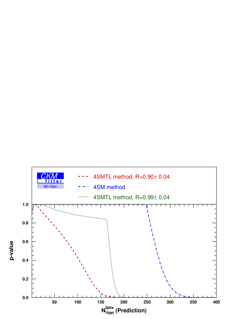
Figure 1: Prediction of the event yield $N_{1bjet}^{2jets}$ as discussed in the text. Blue dotted-dashed line: ‘4SM method’. Red dashed line: ‘4SMTL method’, $i.e.$ applying the tree-level constraints on $|V_{ud}|$, $|V_{us}|$, $|V_{ub}|$, $|V_{cd}|$, $|V_{cb}|$, and ${\cal{B}}(W\rightarrow\ell\nu_{\ell})$ in a the 4SM scenario as explained in the text. Green-dotted line: ‘4SMTL method’ assuming a different $R$ measurement ($R=0.99\pm 0.04$).

The corresponding result (blue dotted-dashed line) shows that the yield could vary a lot with respect to the 3SM value of 142.8 events. However, when taking as inputs the constraints from $|V_{ud}|$, $|V_{us}|$, $|V_{ub}|$, $|V_{cd}|$, $|V_{cb}|$, and on the leptonic branching fractions of $W$-bosons, the expected yield (red dashed line in Fig. 1) clearly prefers smaller values although the 3SM value of 142.8 is still allowed.

The single top cross section measured by CDF gives a measured event yield of $N_{1bjet}^{2jets}=84.3\pm 26.8$, in reasonable agreement with the prediction in the ‘4SMTL method’. Please note that a larger central value for $|V_{cs}|$ as favoured by leptonic $D_{s}$ decays would favour small $N_{1bjet}^{2jets}$ values even stronger since in this case the upper limit on $|V_{ts}|$ would shift towards smaller values.

For a comparison we also present the predicted event yield in the ‘4SMTL method’ (Fig. 1, green dotted line) under the assumption of a hypothetical $R$ value much closer to one: $R=0.99\pm 0.04$. In this case, event yields as large or even slightly larger than the 3SM expectation are possible in the ‘4SMTL method’. In other words, the small single top yield of the CDF analysis and the $R=0.90\pm 0.04$ result of D0 can be accommodated within the ‘4SMTL method’ while the other, large single top cross section results are difficult to explain in a ‘4SMTL method’ with a $R$ value significantly smaller than one.

4.2 Numerical results with the current inputs

With the numerical inputs from Sec. 3 we obtain constraints on $|V_{tb}|$ as shown in Fig. 2. The black dashed-dotted curve shows the p-value as a function of $|V_{tb}|$ for the ‘$R=1$ method’ that neglects $d$- and $s$-quark contributions in single top production and top-quark decay.
The red dashed curve shows the constraint from the ‘3SM method’ using the measured value of $R$. Compared to the ‘$R=1$ method’ the constraint on $|V_{tb}|$ is much stronger in the ‘3SM method’. This might look odd at first glance because $R$ carries now an experimental uncertainty. However, in the ‘3SM method’, not only the single top yield but also $R$ itself provides a constraint on $|V_{tb}|$ thanks to $3\times 3$ unitarity of the CKM matrix. The experimental information from $R$ is much more constraining than the measured value for the single top yield used in our analysis. The preferred value is $|V_{tb}|=0.95$ and $|V_{tb}|=1$ is disfavoured as a result of the $2.5~{}\sigma$ deviation of $R$ from $1$. The blue dashed-dotted curve shows the constraint within the ‘4SM method’ which turns out to be much less constraining than the one obtained in the ‘$R=1$ method’.

Once the tree-level measurements of $|V_{ud}|$, $|V_{us}|$, $|V_{ub}|$, $|V_{cd}|$, $|V_{cb}|$, and the measurements of ${\cal{B}}(W\rightarrow\ell\nu_{\ell})$ are added (‘4SMTL method’), the constraint on $|V_{tb}|$ (green dotted line) becomes much tighter and even tighter than the one from the ‘$R=1$ method’. Due to the deviation of the measured $R$ value from one the 4SMTL constraint is significantly shifted with respect to the standard $|V_{tb}|$ value.

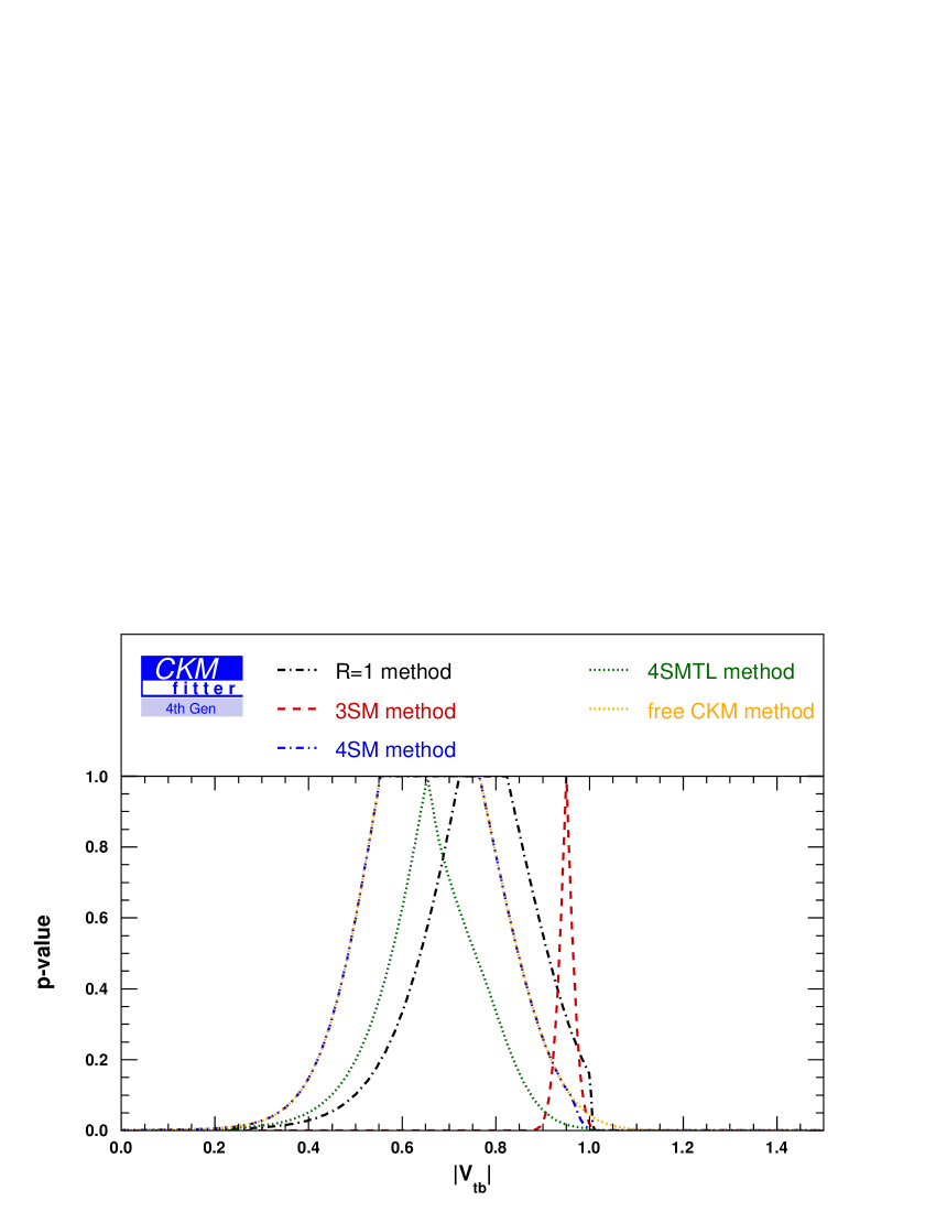
Figure 2: Constraint on $|V_{tb}|$ from the single top analysis within different scenarios using $N_{1bjet}^{2jets}=84.3\pm 26.8$: black dashed-dotted curve: p-value obtained in the ‘$R=1$ method’; red dashed curve: p-value obtained in the ‘3SM method’ setting $R=0.90\pm 0.04$; blue dashed-dotted curve: p-value obtained in the ‘4SM method’ setting $R=0.90\pm 0.04$; green dotted curve: p-value obtained in the ‘4SMTL method’ setting $R=0.90\pm 0.04$ and using in addition constraints on $|V_{ud}|$, $|V_{us}|$, $|V_{ub}|$, $|V_{cd}|$, $|V_{cb}|$, and ${\cal{B}}(W\rightarrow\ell\nu_{\ell})$; orange dotted curve: p-calue obtained in the ‘free CKM method’ setting $R=0.90\pm 0.04$.

We also present the constraints on $|V_{td}|$ and $|V_{ts}|$ in Figs. 3 and 4.

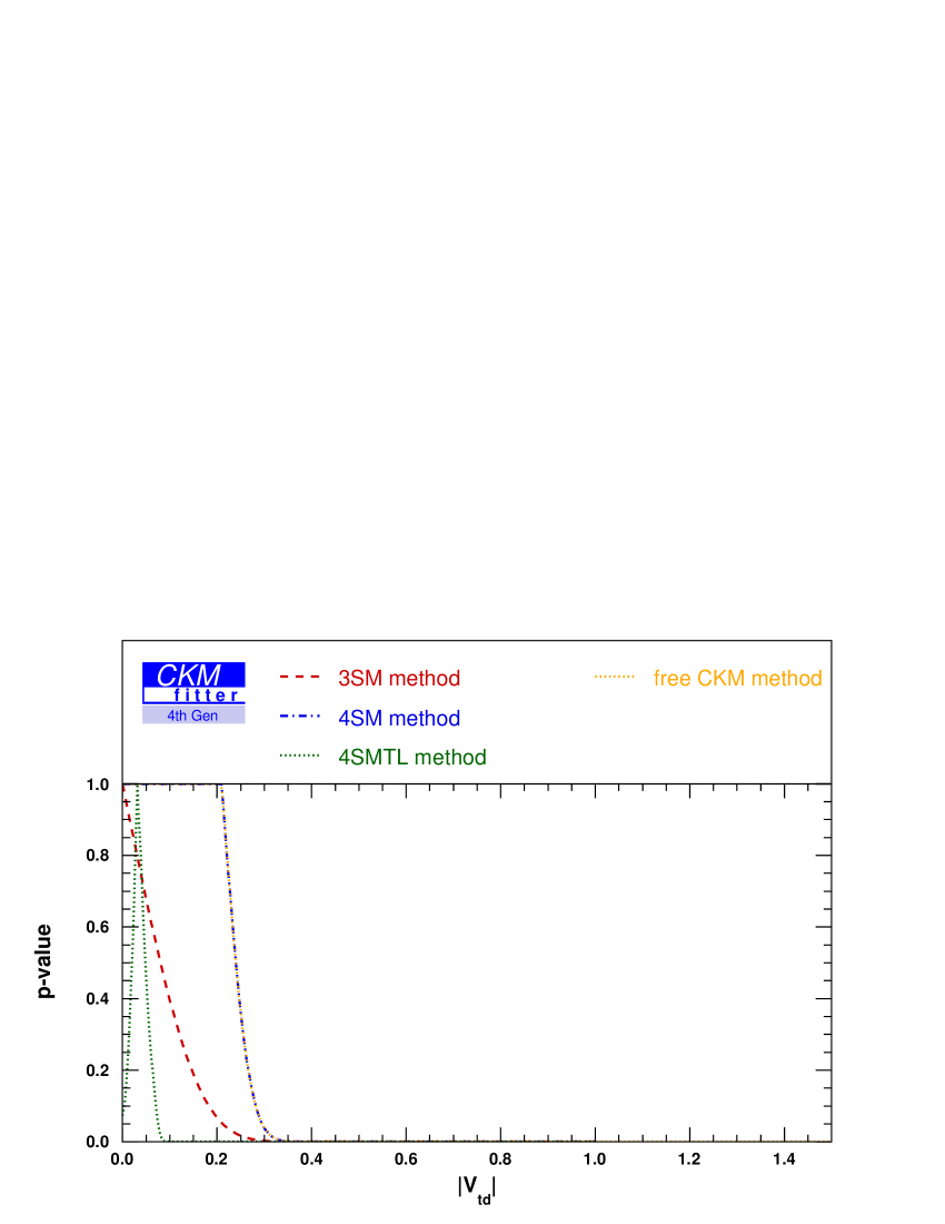
Figure 3: Constraint on $|V_{td}|$ from the single top analysis within different scenarios using $N_{1bjet}^{2jets}=84.3\pm 26.8$. For the different colour-coding we refer to the caption of Fig. 2.

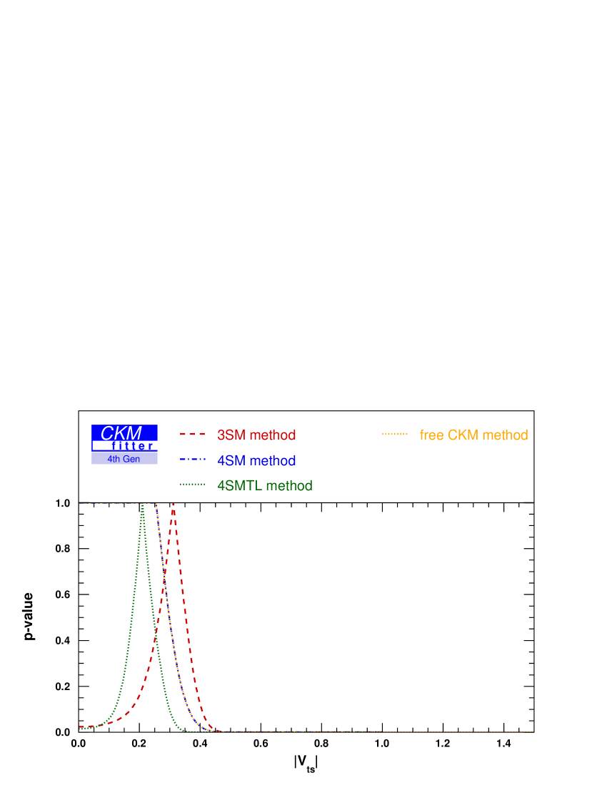
Figure 4: Constraint on $|V_{ts}|$ from the single top analysis within different scenarios using $N_{1bjet}^{2jets}=84.3\pm 26.8$. For the different colour-coding we refer to the caption of Fig. 2.

Figs. 3 and 4 show the corresponding constraints on $|V_{td}|$ and $|V_{ts}|$. In this case, the ‘$R=1$ method’ does not appear as, by definition, both CKM elements are forced to be zero.
To understand better the constraints on $|V_{td}|$ and $|V_{ts}|$ it is instructive to study the correlations between the constraints on $|V_{td}|$, $|V_{ts}|$, and $|V_{tb}|$. In Figs. 5, 6, and 7, we show two-dimensional constraints for the ‘4SM method’. The ring-like constraint in the $|V_{td}|$-$|V_{ts}|$ plane is driven by the $R$ measurement. One does not obtain though a perfect circular shape as the single top yield has different sensitivities to $|V_{td}|$ and $|V_{ts}|$ due to the different sizes of the $t$-channel cross sections and efficiencies. For the same reason, the $|V_{td}|$-$|V_{tb}|$ plane shows an anti-correlation and the $|V_{ts}|$-$|V_{tb}|$ a correlation.

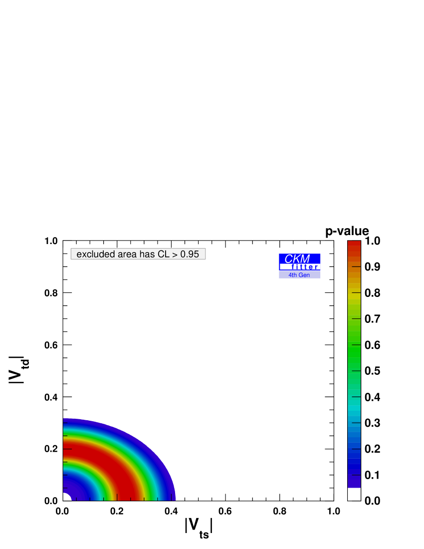
Figure 5: The two-dimensional constraint on $|V_{td}|$ as a function of $|V_{ts}|$ within the ‘4SM method’ from the single top analysis using $N_{1bjet}^{2jets}=84.3\pm 26.8$ and $R=0.90\pm 0.04$.

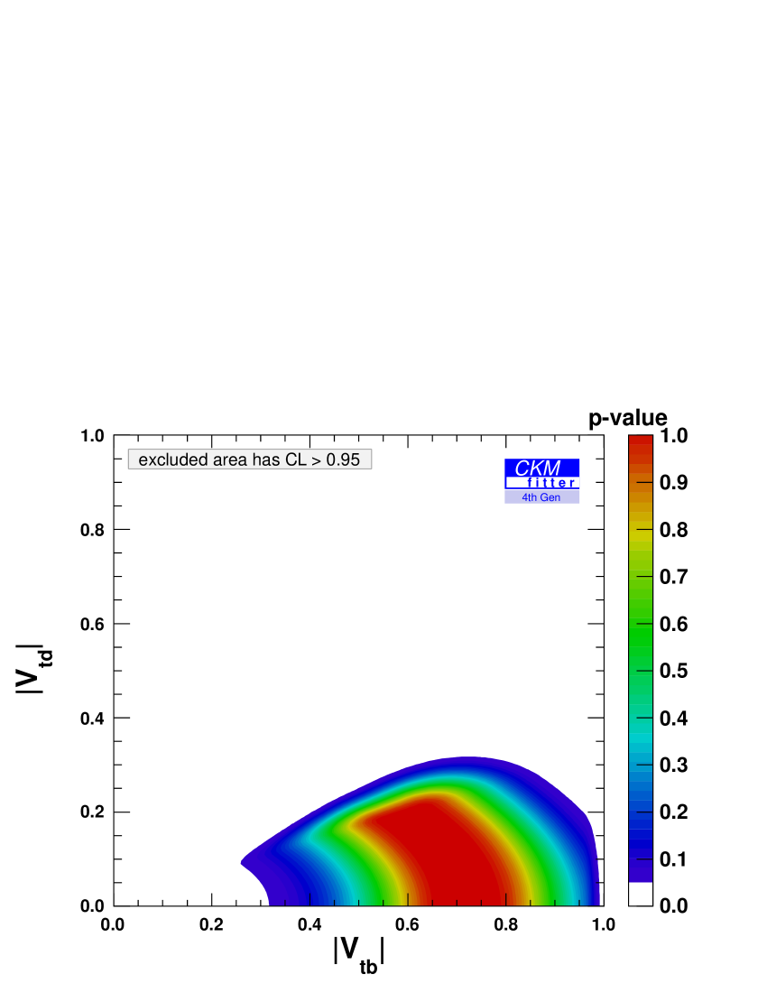
Figure 6: The two-dimensional constraint on $|V_{td}|$ as a function of $|V_{tb}|$ within the ‘4SM method’ from the single top analysis using $N_{1bjet}^{2jets}=84.3\pm 26.8$ and $R=0.90\pm 0.04$.

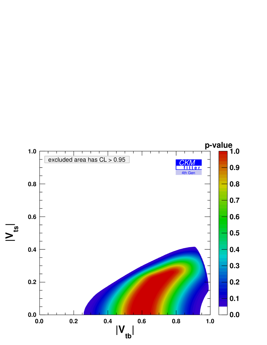
Figure 7: The two-dimensional constraint on $|V_{ts}|$ as a function of $|V_{tb}|$ within the ‘4SM method’ from the single top analysis using $N_{1bjet}^{2jets}=84.3\pm 26.8$ and $R=0.90\pm 0.04$.

In Figs. 8, 9, and 10 we present the corresponding constraints in the ‘4SMTL method’. Due to the very precisely measured value of $|V_{ud}|$, the allowed values of $|V_{td}|$ are well-constrained to be below $0.08$. As a consequence, the devation of $R$ from 1 can only be compensated by a rather large value of $|V_{ts}|$ of order 0.21 which is still allowed by the unitarity constraints in the second column of the $4\times 4$ CKM matrix but not preferred.

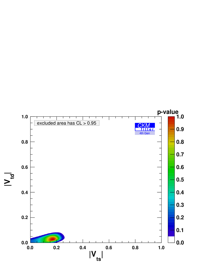
Figure 8: The two-dimensional constraint on $|V_{td}|$ and $|V_{ts}|$ within the ‘4SMTL method’ using $N_{1bjet}^{2jets}=84.3\pm 26.8$ and $R=0.90\pm 0.04$ together with constraints on $|V_{ud}|$, $|V_{us}|$, $|V_{ub}|$, $|V_{cd}|$, $|V_{cb}|$, and ${\cal{B}}(W\rightarrow\ell\nu_{\ell})$ as explained in the text.

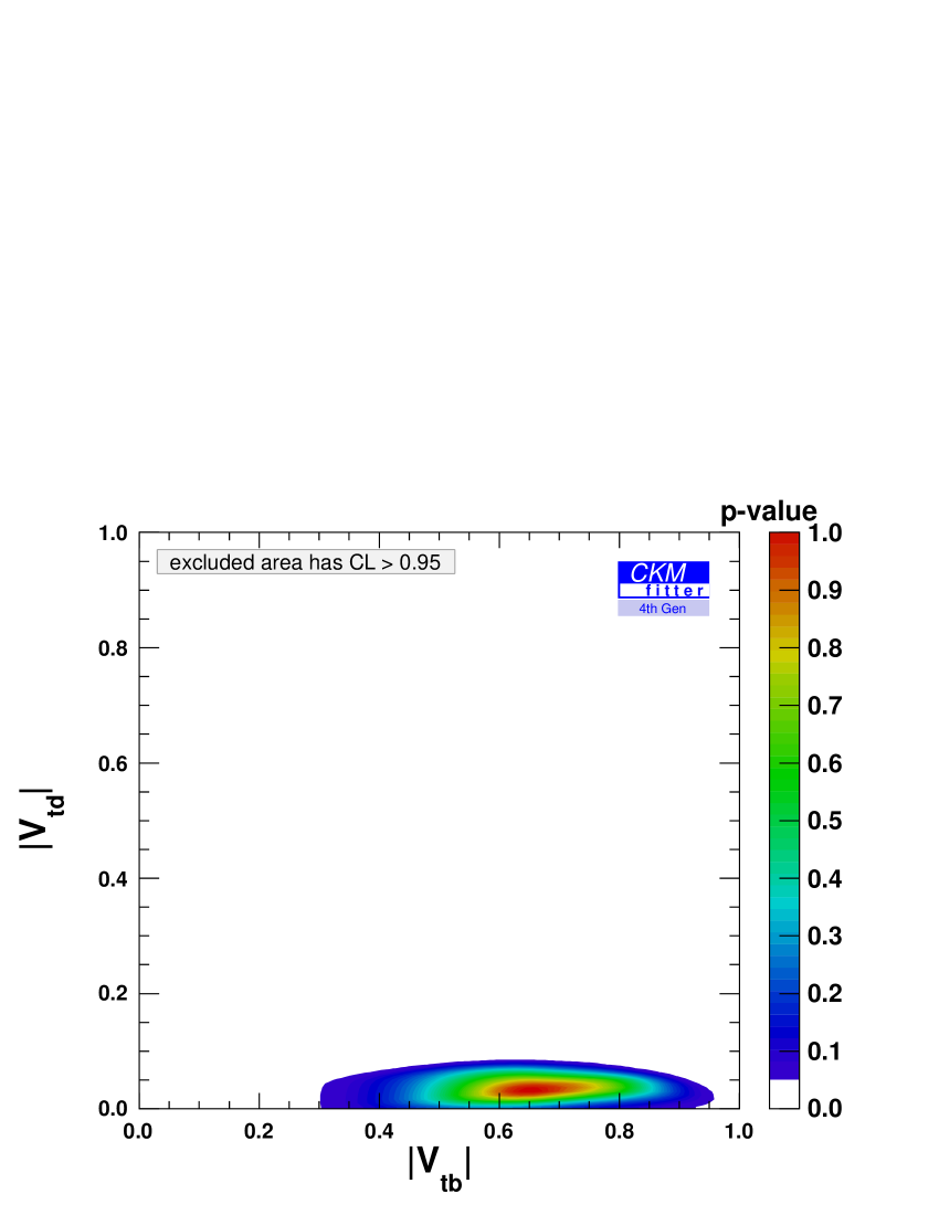
Figure 9: The two-dimensional constraint on $|V_{td}|$ and $|V_{tb}|$ within the ‘4SMTL method’ using $N_{1bjet}^{2jets}=84.3\pm 26.8$ and $R=0.90\pm 0.04$ together with constraints on $|V_{ud}|$, $|V_{us}|$, $|V_{ub}|$, $|V_{cd}|$, $|V_{cb}|$, and ${\cal{B}}(W\rightarrow\ell\nu_{\ell})$ as explained in the text.

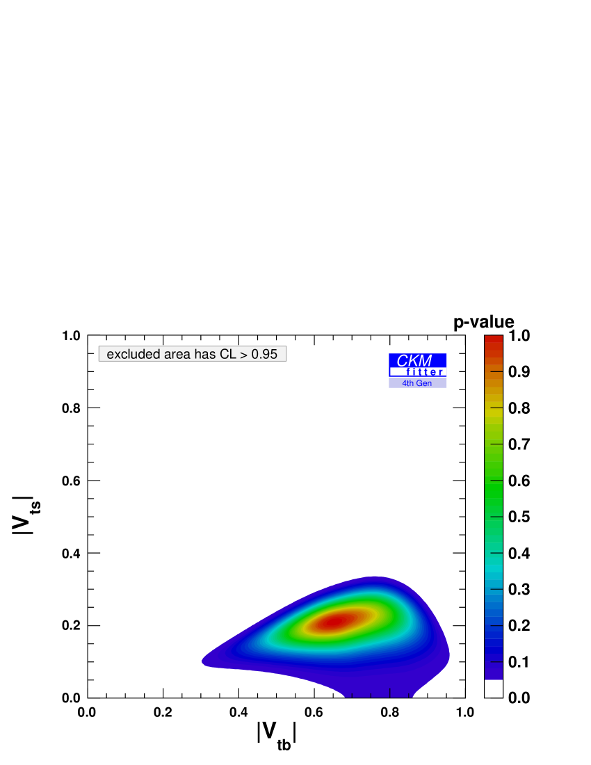
Figure 10: The two-dimensional constraint on $|V_{ts}|$ and $|V_{tb}|$ within the ‘4SMTL method’ using $N_{1bjet}^{2jets}=84.3\pm 26.8$ and $R=0.90\pm 0.04$ together with constraints on $|V_{ud}|$, $|V_{us}|$, $|V_{ub}|$, $|V_{cd}|$, $|V_{cb}|$, and ${\cal{B}}(W\rightarrow\ell\nu_{\ell})$ as explained in the text.

Next, we study the constraints in a hypothetical scenario where the measured single top yield is in perfect agreement with the expected number of signal events in the 3SM scenario assuming $|V_{tb}|=1$ but still using the measured $R$ value. In this hypothetical scenario we set $N_{1bjet}^{2jets}=142.8\pm 34.6$. The corresponding plot for the constraint on $|V_{tb}|$ is shown in Fig. 11. In this case, although the measured single top yield perfectly fits with the 3SM expectation the $|V_{tb}|$ constraints in the 3SM, 4SM and even ‘4SMTL method’s still deviate significantly from the standard scenario.

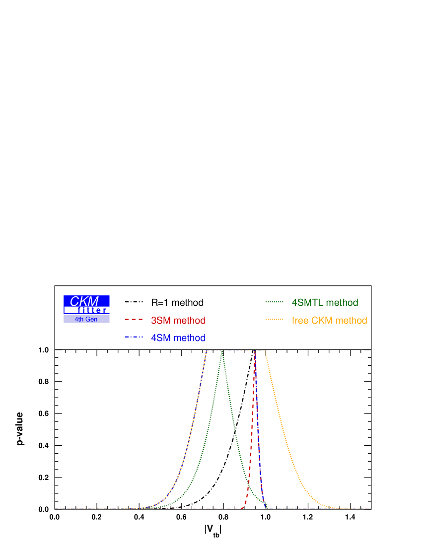
Figure 11: Constraint on $|V_{tb}|$ from a single top analysis assuming a hypothetical measurement of $N_{1bjet}^{2jets}=142.8\pm 34.6$: black dashed-dotted curve: p-value obtained in the ‘$R=1$ method’; red dashed curve: p-value obtained in the ‘3SM method’ setting $R=0.90\pm 0.04$; blue dashed-dotted curve: p-value obtained in the ‘4SM method’ setting $R=0.90\pm 0.04$; green dotted curve: p-value obtained in the ‘4SMTL method’ setting $R=0.90\pm 0.04$ and using in addition constraints on $|V_{ud}|$, $|V_{us}|$, $|V_{ub}|$, $|V_{cd}|$, $|V_{cb}|$, and ${\cal{B}}(W\rightarrow\ell\nu_{\ell})$; orange dotted curve: p-calue obtained in the ‘free CKM method’ setting $R=0.90\pm 0.04$.

4.3 Numerical results with a modified $R$ input

We now perform an instructive exercise. As the new $R$ measurement from D0 leads to a large $\chi^{2}$ value in the 4SM fit when combined with tree-level constraints and the single top measurements we modify the central value of $R$ such that one obtains a reasonably small $\chi^{2}$, that is, the $R$ measurement would be in agreement with the tree-level constraints and the measured single top yield. We choose $R=0.99\pm 0.04$ and present the $|V_{tb}|$ constraint in Figs. 12 and 13 corresponding to measured event yields of $N_{1bjet}^{2jets}=84.3\pm 26.8$, respectively, $N_{1bjet}^{2jets}=142.8\pm 34.6$.

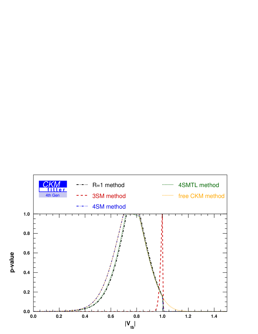
Figure 12: Constraint on $|V_{tb}|$ from a single top analysis using $N_{1bjet}^{2jets}=84.3\pm 26.8$: black dashed-dotted curve: p-value obtained in the ‘$R=1$ method’; red dashed curve: p-value obtained in the ‘3SM method’ setting $R=0.99\pm 0.04$; blue dashed-dotted curve: p-value obtained in the ‘4SM method’ setting $R=0.99\pm 0.04$; green dotted curve: p-value obtained in the ‘4SMTL method’ setting $R=0.99\pm 0.04$ and using in addition constraints on $|V_{ud}|$, $|V_{us}|$, $|V_{ub}|$, $|V_{cd}|$, $|V_{cb}|$, and ${\cal{B}}(W\rightarrow\ell\nu_{\ell})$; orange dotted curve: p-calue obtained in the ‘free CKM method’ setting $R=0.99\pm 0.04$.

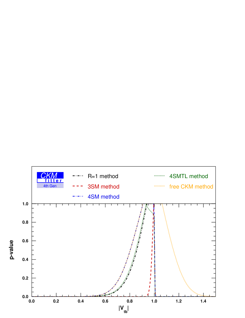
Figure 13: Constraint on $|V_{tb}|$ from a single top analysis assuming hypothetical measurement $N_{1bjet}^{2jets}=142.8\pm 34.6$: black dashed-dotted curve: p-value obtained in the ‘$R=1$ method’; red dashed curve: p-value obtained in the ‘3SM method’ setting $R=0.99\pm 0.04$; blue dashed-dotted curve: p-value obtained in the ‘4SM method’ setting $R=0.99\pm 0.04$; green dotted curve: p-value obtained in the ‘4SMTL method’ setting $R=0.99\pm 0.04$ and using in addition constraints on $|V_{ud}|$, $|V_{us}|$, $|V_{ub}|$, $|V_{cd}|$, $|V_{cb}|$, and ${\cal{B}}(W\rightarrow\ell\nu_{\ell})$; orange dotted curve: p-calue obtained in the ‘free CKM method’ setting $R=0.99\pm 0.04$.

Once $R$ is very close to one the difference in the constraints on $|V_{tb}|$ between the ‘$R=1$ method and the ‘4SM(TL) method’ becomes small (tiny).

4.4 The top-quark decay width

Under the assumption that the top-quark decays have to proceed through $t\rightarrow q+W$, $q=d,s,b$, the total top-quark decay width for massless final-state quarks at NLO in QCD is given by [46]

$$\Gamma_{t} = (|V_{td}|^{2}+|V_{ts}|^{2}+|V_{tb}|^{2})\frac{G_{F}m_{t}^{3}}{8\pi\sqrt{2}}(1-\frac{m_{W}^{2}}{m_{t}^{2}})^{2}(1+2\frac{m_{W}^{2}}{m_{t}^{2}})$$ (13)

$$\times \left[1-\frac{2\alpha_{s}}{3\pi}(\frac{2\pi^{2}}{3}-\frac{5}{2})\right],$$

where $G_{F}=1.16637\cdot 10^{-5}\,{\rm GeV}^{-2}$ [31] is the Fermi constant, and the QCD corrections are included in the $m_{W}/m_{t}\ll 1$ limit.

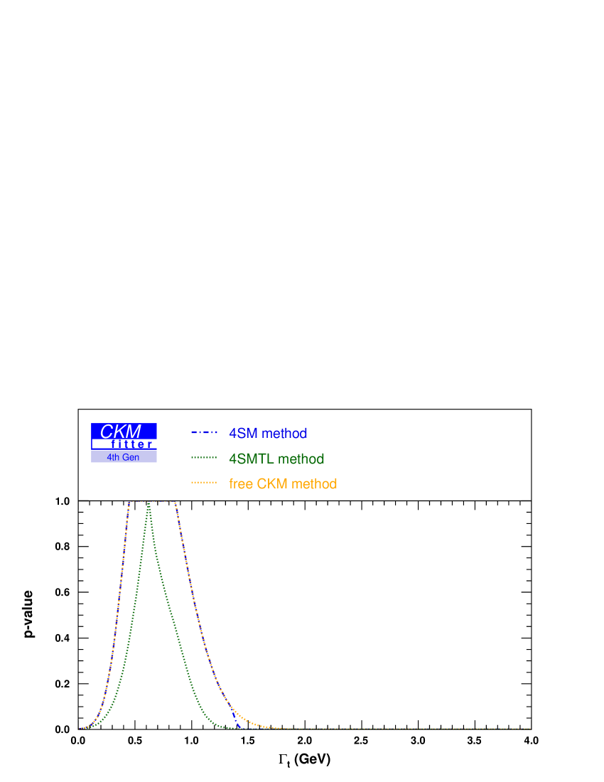
Figure 14: Constraint on $\Gamma_{t}$ from a single top analysis assuming hypothetical measurement $N_{1bjet}^{2jets}=84.3\pm 26.8$: blue dashed-dotted curve: p-value obtained in the ‘4SM method’ setting $R=0.90\pm 0.04$; green dotted curve: p-value obtained in the ‘4SMTL method’ setting $R=0.90\pm 0.04$ and using in addition constraints on $|V_{ud}|$, $|V_{us}|$, $|V_{ub}|$, $|V_{cd}|$, $|V_{cb}|$, and ${\cal{B}}(W\rightarrow\ell\nu_{\ell})$; orange dotted curve: p-calue obtained in the ‘free CKM method’ setting $R=0.90\pm 0.04$.

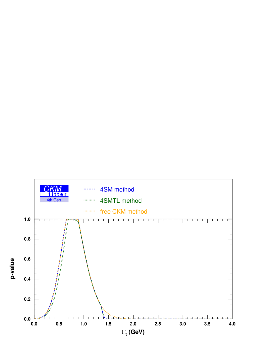
Figure 15: Constraint on $\Gamma_{t}$ from a single top analysis assuming hypothetical measurement $N_{1bjet}^{2jets}=84.3\pm 26.8$: blue dashed-dotted curve: p-value obtained in the ‘4SM method’ setting $R=0.99\pm 0.04$; green dotted curve: p-value obtained in the ‘4SMTL method’ setting $R=0.99\pm 0.04$ and using in addition constraints on $|V_{ud}|$, $|V_{us}|$, $|V_{ub}|$, $|V_{cd}|$, $|V_{cb}|$, and ${\cal{B}}(W\rightarrow\ell\nu_{\ell})$; orange dotted curve: p-calue obtained in the ‘free CKM method’ setting $R=0.99\pm 0.04$.

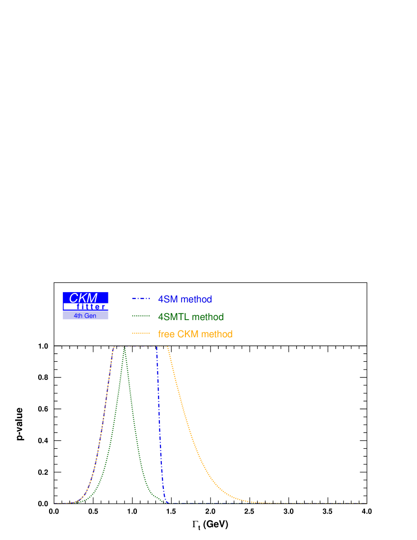
Figure 16: Constraint on $\Gamma_{t}$ from a single top analysis assuming hypothetical measurement $N_{1bjet}^{2jets}=142.8\pm 34.6$: blue dashed-dotted curve: p-value obtained in the ‘4SM method’ setting $R=0.90\pm 0.04$, green dotted curve: p-value obtained in the ‘4SMTL method’ setting $R=0.90\pm 0.04$ and using in addition constraints on $|V_{ud}|$, $|V_{us}|$, $|V_{ub}|$, $|V_{cd}|$, $|V_{cb}|$, and ${\cal{B}}(W\rightarrow\ell\nu_{\ell})$; orange dotted curve: p-calue obtained in the ‘free CKM method’ setting $R=0.90\pm 0.04$.

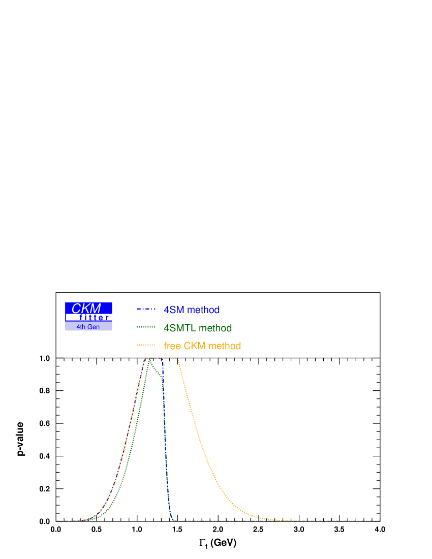
Figure 17: Constraint on $\Gamma_{t}$ from a single top analysis assuming hypothetical measurement $N_{1bjet}^{2jets}=142.8\pm 34.6$: blue dashed-dotted curve: p-value obtained in the ‘4SM method’ setting $R=0.99\pm 0.04$; green dotted curve: p-value obtained in the ‘4SMTL method’ setting $R=0.99\pm 0.04$ and using in addition constraints on $|V_{ud}|$, $|V_{us}|$, $|V_{ub}|$, $|V_{cd}|$, $|V_{cb}|$, and ${\cal{B}}(W\rightarrow\ell\nu_{\ell})$; orange dotted curve: p-calue obtained in the ‘free CKM method’ setting $R=0.99\pm 0.04$.

In the 3SM, $|V_{td}|^{2}+|V_{ts}|^{2}+|V_{tb}|^{2}$ is equal to one due to unitarity and one predicts the top-quark width to be $\Gamma_{t}=(1.32\pm 0.04)\,{\rm GeV}$ where we have used $\alpha_{s}=0.118$, $m_{W}=80.399~{}{\rm GeV}$ for the $W$-boson mass, and $m_{t}=(172.0\pm 1.6)\,{\rm GeV}$ for the top-quark mass as in our numerical analysis.
In Figs. 14, 15, 16, and 17, we present the constraints on $\Gamma_{t}$ obtained in the ‘4SM method’, ‘4SMTL method’, and the ‘free CKM method’ respectively. The latter method can be considered the closest to that employed by the D0 collaboration to extract $\Gamma_{t}$. The constraints are determined for the different values of $R$ and $N_{1bjet}^{2jets}$ used in the numerical analyses described above. As expected, the constraints on $\Gamma_{t}$ are identical for the ‘4SM method’ and the ‘free CKM method’ for values of $\Gamma_{t}$ below the 3SM expectation of $\Gamma_{t}=1.32{\rm GeV}$ as this is the allowed region of $\Gamma_{t}$ for $|V_{td}|^{2}+|V_{ts}|^{2}+|V_{tb}|^{2}\leq 1$.
Analoguous to the $|V_{tq}|$ constraints the differences between the ‘4SM method’ and the ‘4SMTL method’ turn out to be significant for $R=0.90\pm 0.04$.

5 Conclusion

We have presented a strategy to extract the CKM matrix elements $|V_{tb}|$ and also $|V_{td}|$ and $|V_{ts}|$ from single top production measurements at the Tevatron which goes beyond the ‘$R=1$ method’ assuming $|V_{tb}|\gg|V_{td}|,|V_{ts}|$, and explicitely takes into account $d$- and $s$-quark contributions to the $s$- and $t$-channel production and to the decay of top quarks. The method provides information that can be directly used to put constraints on 4SM and other scenarios with new heavy quarks and to extract the top-quark width within these scenarios.

For sake of illustration, we applied the method to CDF data on lepton $+$ missing transverse energy $+$ two jet events with one reconstructed $b$-jet and to recent D0 results on the top branching ratio to $b$-quarks. We estimated the relevant efficiencies from a leading order Monte-Carlo simulation. The constraints within a 4SM scenario from the single top measurements and from $R$ can only be combined with other flavor observables in a consistent way within a global analysis. As an example, we studied a global analysis of the single top yield $N_{1bjet}^{2jets}$ and $R$ with tree-level flavor measurements to constrain CKM matrix elements in a 4SM scenario.

Our simplified analysis shows that with the recent measurement of $R=0.90\pm 0.04$ presented by the D0 collaboration the constraint on $|V_{tb}|$ in a 4SM scenario differs significantly from the ‘$R=1$ method’ even if $|V_{td}|$ and $|V_{ts}|$ are constrained by tree-level measurements of $|V_{ud}|$, $|V_{us}|$, $|V_{ub}|$, $|V_{cd}|$, $|V_{cb}|$, and by leptonic $W$-decays thanks to $4\times 4$ unitarity.

Further valuable and accurate information could be easily extracted from the Tevatron data by including also event rates with two or three jets, both of them $b$-tagged and by employing NLO MC + data validation for the determination of the efficiencies. In particular, the fact that $s$-channel and $t$-channel at the Tevatron are expected to give comparable rates of events in the SM provides a leverage that has no equivalent at the LHC and put CDF and D0 in a very competitive position.

While this paper concentrates on single top-quark production we would like to point out that a value of $R$ being significantly smaller than one might have important implications for $t\bar{t}$ production measurements. Without taking into account $R$ being smaller than one, the measured $t\bar{t}$ cross section would underestimate the true cross-section value which in turn would overestimate the top-quark mass extracted from the cross section measurement. As an example, if a $t\bar{t}$ cross-section measurement performed at Tevatron used one b-tagged jet, then the cross section would be underestimated by a factor $R$. Correspondingly, the extracted top-quark mass would be overestimated by about $O(3~{}{\rm GeV})$ which can be read off e.g. from Ref. [47] where the top-quark mass extraction from $t\bar{t}$ cross-section measurements is discussed in detail. This issue might become relevant when comparing the top-quark mass extracted from a cross-section measurement with the one from direct measurements.

The method outlined in this work can also be applied to single top-quark measurements at the LHC. In this case, however, $s$-channel single top production is very small, while $Wt$ associated production becomes visible and therefore could be included. Furthermore, at the LHC the $t$-channel rate of top and anti-top is different due to the $pp$ initial state, $d$’s are valence (+sea) quarks while $\bar{d}$ are only sea quarks. Contributions of the $d$ from the $s$ contributions could therefore be singled out by an accurate charge asymmetry measurement. Rapidity distributions could also provide a further handle [48]. At LHC, however, one expects a lower sensitivity to $d$- and $s$-contributions since the $t$-channel cross sections for $d$- and $s$-contributions do not differ from the $b$-contribution as much as at the Tevatron. As an example, we quote for a center-of-mass energy of $8~{}{\rm TeV}$ the NLO cross-sections of single top and single antitop production at the LHC in Tables 4 and 5 calculated as the ones for Tevatron described in Sec. 3.1.

Cross section	value	PDF unc.	scale unc.
	[pb]	[pb]	[pb]
$\sigma_{d}^{t}$	$396.3$	$\pm 15.1$	${}^{+2.8}_{-1.2}$
$\sigma_{s}^{t}$	$124.9$	$\pm 7.4$	${}^{+1.5}_{-0.6}$
$\sigma_{b}^{t}$	$54.8$	$\pm 0.7$	${}^{+1.8}_{-1.0}$

Table 4: NLO cross section for $t$-channel single top production at the LHC for a center-of-mass energy $\sqrt{s}=8~{}{\rm TeV}$ calculated with MCFM [32] using the PDF sets taken from MSTW2008 [33].

Cross section	value	PDF unc.	scale unc.
	[pb]	[pb]	[pb]
$\sigma_{d}^{t}$	$108.9$	$\pm 5.0$	${}^{+1.5}_{-0.1}$
$\sigma_{s}^{t}$	$69.6$	$\pm 3.5$	${}^{+1.2}_{-0.3}$
$\sigma_{b}^{t}$	$30.0$	$\pm 0.6$	${}^{+0.9}_{-0.7}$

Table 5: NLO cross section for $t$-channel single anti-top production at the LHC for a center-of-mass energy $\sqrt{s}=8~{}{\rm TeV}$ calculated with MCFM [32] using the PDF sets taken from MSTW2008 [33].

Finally, the measurements suggested and outlined here provide complementary and assumption-free constraints that can be used and combined to those obtained via direct searches of a fourth generation and/or precision observables. Work in this direction is in progress.

References

- [1] N. Cabibbo, “Unitary Symmetry and Leptonic Decays,” Phys. Rev. Lett. 10, 531 (1963); M. Kobayashi and T. Maskawa, “CP Violation in the Renormalizable Theory of Weak Interaction,” Prog. Theor. Phys. 49, 652 (1973).
- [2] The CKMfitter Group (J. Charles et al.), Eur. Phys. J. C 41, 1 (2005), updated at http://ckmfitter.in2p3.fr/.
- [3] The CKMfitter Group (J. Charles et al.), Phys. Rev. D 84 (2011) 033005 [arXiv:1106.4041 [hep-ph]].
- [4] J. Alwall et al., Eur. Phys. J. C 49 (2007) 791
- [5] V. M. Abazov et al. (D0 collaboration), Phys. Rev. Lett. 100, 192003 (2008)
- [6] V. M. Abazov et al. (D0 collaboration), arXiv:1106.5436 [hep-exp], Phys. Rev. Lett. 107, 121802 (2011)
- [7] M. S. Chanowitz, Phys. Rev. D 82 (2010) 035018 [arXiv:1007.0043 [hep-ph]]; M. S. Chanowitz, Phys. Rev. D 79 (2009) 113008 [arXiv:0904.3570 [hep-ph]].
- [8] O. Eberhardt, A. Lenz and J. Rohrwild, Phys. Rev. D 82 (2010) 095006 [arXiv:1005.3505 [hep-ph]].
- [9] A. K. Alok, A. Dighe and D. London, Phys. Rev. D 83 (2011) 073008 [arXiv:1011.2634 [hep-ph]].
- [10] A. Lister [CDF Collaboration], “Search for Heavy Top-like Quarks tprime-¿Wq Using Lepton Plus Jets Events in 1.96 TeV pbar Collisions,” arXiv:0810.3349 [hep-ex]; J. Conway [CDF Collaboration], CDF public conference note CDF/PUB/TOP/PUBLIC/10110
- [11] The ATLAS Collaboration, “Search for pair-produced heavy quarks decaying to Wq in the two-lepton channel at sqrt(s) = 7 TeV with the ATLAS detector,” arXiv:1202.3389 [hep-ex].
- [12] The ATLAS Collaboration, “Search for pair production of a heavy quark decaying to a W boson and a b quark in the lepton+jets channel with the ATLAS detector,” arXiv:1202.3076 [hep-ex].
- [13] The ATLAS collaboration, “Search for Fourth Generation Quarks Decaying to in pp collisions at with the ATLAS Detector”, ATLAS-CONF-2011-022.
- [14] The CMS collaboration, “Search for a Heavy Top-like Quark in the Dilepton Final State in pp collisions at ”, CMS-PAS-EXO-11-050
- [15] The CMS collaboration, “Search for t’ pair production in lepton+jets channel”, CMS-PAS-EXO-11-051
- [16] T. Aaltonen et al. [CDF Collaboration], Phys. Rev. Lett. 104 (2010) 091801 [arXiv:0912.1057 [hep-ex]].
- [17] T. Aaltonen et al. [The CDF Collaboration], Phys. Rev. Lett. 106 (2011) 141803 [arXiv:1101.5728 [hep-ex]].
- [18] G. Aad et al. [ATLAS Collaboration], “Inclusive search for same-sign dilepton signatures in pp collisions at with the ATLAS detector,” arXiv:1108.0366 [hep-ex].
- [19] The CMS collaboration, “Search for a Heavy Bottom-like Quark in pp Collisions at ”, CMS-PAS-EXO-11-036
- [20] The CMS collaboration, “Inclusive search for a fourth generation of quarks with the CMS experiment” CMS-PAS-EXO-11-054
- [21] B. W. Harris et al. Phys. Rev. D 66 (2002) 054024
- [22] J. Campbell, K. Ellis, and F. Tramontano, Phys. Rev. D 70 (2004) 094012.
- [23] N. Kidonakis, Phys. Rev. D 81, 054028 (2010) [arXiv:1001.5034 [hep-ph]].
- [24] J. M. Campbell, R. Frederix, F. Maltoni and F. Tramontano, JHEP 0910 (2009) 042 [arXiv:0907.3933 [hep-ph]].
- [25] J. M. Campbell, R. Frederix, F. Maltoni and F. Tramontano, Phys. Rev. Lett. 102 (2009) 182003 [arXiv:0903.0005 [hep-ph]].
- [26] T. Sjöstrand et al., Computer Phys. Commun. 135 (2001) 238, [arXiv: hep-ph/0010017]
- [27] S. Frixione and B. R. Webber, JHEP 0206:029,2002
- [28] P. Nason, JHEP 0411:040,2004
- [29] S. Frixione, E. Laenen, P. Motylinski, B. R. Webber, JHEP 0603, 092 (2006). [hep-ph/0512250].
- [30] S. Alioli, P. Nason, C. Oleari, E. Re, JHEP 0909, 111 (2009). [arXiv:0907.4076 [hep-ph]].
- [31] K. Nakamura et al. [Particle Data Group], J. Phys. G 37 (2010) 075021.
- [32] J. Campbell and K. Ellis, “MCFM - Monte Carlo for FeMtobarn processes”, http://mcfm.fnal.gov/
- [33] A. D. Martin, W. J. Stirling, R. S. Thorne and G. Watt, “Parton distributions for the LHC,” Eur. Phys. J. C 63 (2009) 189 [arXiv:0901.0002 [hep-ph]].
- [34] T. Aaltonen et al. [CDF Collaboration], Phys. Rev. Lett. 103 (2009) 092002 [arXiv:0903.0885 [hep-ex]].
- [35] T. Aaltonen et al. [CDF Collaboration], Phys. Rev. D 82 (2010) 112005 [arXiv:1004.1181 [hep-ex]].
- [36] H. Lacker and A. Menzel, “Simultaneous Extraction of the Fermi constant and PMNS matrix elements in the presence of a fourth generation,” JHEP 1007 (2010) 006 [arXiv:1003.4532 [hep-ph]].
- [37] J. C. Hardy and I. S. Towner, Phys. Rev. C 79 (2009) 055502
- [38] M. Antonelli et al., Eur. Phys. J. C 69 (2010) 399 [arXiv:1005.2323 [hep-ph]].
- [39] A. Lenz et al., Phys. Rev. D 83 (2011) 036004, [arXiv:1008.1593 [hep-ph]].
- [40] E. Barberio et al. [Heavy Flavour Averaging Group], [arXiv:0808.1297 [hep-ex]] and online update at http://www.slac.stanford.edu/xorg/hfag updated for PDG 2009.
- [41] The LEP Collaborations: ALEPH Collaboration, DELPHI Collaboration, L3 Collaboration, OPAL Collaboration, the LEP Electroweak Working Group, “A combination of preliminary electroweak measurements and constraints on the standard model”, [arXiv:hep-ex/0612034v2].
- [42] V. M. Abazov et al. [ D0 Collaboration ], “An improved determination of the width of the top quark,” [arXiv:1201.4156 [hep-ex]].
- [43] V. M. Abazov et al. [ D0 Collaboration ], “Measurements of single top quark production cross sections and in collisions at TeV,” [arXiv:1108.3091 [hep-ex]].
- [44] The ATLAS Collaboration, “Measurement of the t-channel Single-Top Production Cross Section in of pp Collisions at collected with the ATLAS detector”, ATLAS-CONF-2011-101
- [45] The CMS Collaboration, “Measurement of t-channel single-top cross section in pp collisions at ”, CMS PAS TOP-10-008
- [46] M. Jezabek and J. H. Kühn, Nucl. Phys. B 314, 1 (1989)
- [47] U. Langenfeld, S. -O. Moch, P. Uwer, PoS ICHEP2010 (2010) 082.
- [48] J. A. Aguilar-Saavedra and A. Onofre, Phys. Rev. D 83 (2011) 073003 [arXiv:1002.4718 [hep-ph]].