Sweeping Away the Mysteries of Dusty Continuous Winds in AGN

Abstract

An integral part of the Unified Model for Active Galactic Nuclei (AGNs) is an axisymmetric obscuring medium, which is commonly depicted as a torus of gas and dust surrounding the central engine. However, a robust, dynamical model of the torus is required in order to understand the fundamental physics of AGNs and interpret their observational signatures. Here we explore self-similar, dusty disk-winds, driven by both magnetocentrifugal forces and radiation pressure, as an explanation for the torus. Using these models, we make predictions of AGN infrared (IR) spectral energy distributions (SEDs) from $2-100{\,\mu\rm m}$ by varying parameters such as: the viewing angle (from $i=0^{\circ}-90^{\circ}$); the base column density of the wind (from $N_{H,0}=10^{23}-10^{25}$ cm^-2); the Eddington ratio (from $L/L_{Edd}=0.01-0.1$); the black hole mass (from $M_{BH}=10^{8}-10^{9}{\rm\,M_{\odot}}$); and the amount of power in the input spectrum emitted in the X-ray relative to that emitted in the UV/optical (from $\alpha_{ox}=1.1-2.1$). We find that models with $N_{H,0}=10^{25}$ cm^-2, $L/L_{Edd}=0.1$, and $M_{BH}\geq 10^{8}{\rm\,M_{\odot}}$ are able to adequately approximate the general shape and amount of power expected in the IR as observed in a composite of optically luminous Sloan Digital Sky Survey (SDSS) quasars. The effect of varying the relative power coming out in X-rays relative to the UV is a change in the emission below $\sim 5$ µm from the hottest dust grains; this arises from the differing contributions to heating and acceleration of UV and X-ray photons. We see mass outflows ranging from $\sim 1$–4 ${\rm\,M_{\odot}}$ yr^-1, terminal velocities ranging from $\sim 1900$–8000 km sec^-1, and kinetic luminosities ranging from $\sim 1\times 10^{42}$–$8\times 10^{43}$ erg s^-1. Further development of this model holds promise for using specific features of observed IR spectra in AGNs to infer fundamental physical parameters of the systems.

1 Introduction

Active galactic nuclei (AGNs) are often set apart from other astrophysical objects by their powerful spectral energy distributions (SEDs) that radiate a substantial amount of power across the electromagnetic spectrum (e.g., Elvis et al., 1994). In addition to being powerful, AGNs are also a motley lot, known for displaying a wide range of observable characteristics among them. Objects of two types – radio-loud and radio-quiet – have a range of intrinsic luminosities, and may display either only narrow, or both narrow and broad spectral emission lines (Antonucci, 1993).

The Unified Model (e.g., Antonucci, 1993; Urry & Padovani, 1995) is a phenomenological depiction of AGNs that posits that the nature of many of these differences, particularly the presence or absence of broad emission lines, can be explained primarily as a function of viewing angle. Pictured at the core of this model is the “central engine,” composed of the supermassive black hole (with a mass from $\sim 10^{6}$–$10^{9}{\rm\,M_{\odot}}$) and its sub-parsec-scale accretion disk, where matter is heated as it falls towards the black hole. Another key feature of the Unified Model is a structure that surrounds the accretion disk: an axisymmetric, obscuring medium, which covers many lines of sight to the accretion disk around the central black hole. This obscuring medium is commonly depicted as a torus of optically thick dusty gas which can extend up to 100 pc (e.g., Antonucci & Miller, 1985). This dusty torus, which is also the main source of infrared emission in an AGN, can block the accretion disk continuum and broad emission lines produced within the Broad Line Region (BLR) by obscuring them with dusty gas (e.g., Sanders et al., 1989; Barvainis, 1990).

A consequence of this geometry is that when the AGN is viewed face-on, we observe a “Type 1” active galaxy displaying both narrow lines (permitted and forbidden) with line widths of hundreds of km s^-1, as well as the broad lines emanating from the exposed hot ($\sim 10^{5}$ K) and bright photoionized gas around the central accretion disk, with widths of thousands of km s^-1 (Antonucci, 1993). When viewed edge-on, the broad lines are obscured by the optically thick dusty torus, and we observe only the narrow lines generated on much larger scales characteristic of “Type 2” active galaxies.

As a further clue to the structure of the torus, there is observational evidence for a luminosity dependence of the fraction of Type 1 and Type 2 AGNs. For example, in a deep hard X-ray survey, Steffen et al. (2003) show that Type 1 AGNs dominate at higher luminosities, while Type 2 AGNs become an important component of the X-ray population only at lower, Seyfert-like luminosities. Similarly, Hao et al. (2005a) shows that the fraction of Type 1 AGNs increases with luminosity of the [OIII] narrow emission line (see also Simpson 2005), and studies using radio-selected AGN samples consistently point to the same trend (see e.g., Hill et al., 1996; Simpson & Rawlings, 2000; Grimes et al., 2004).

Assuming the inner wall of the torus is set at the radius at which dust sublimates (e.g., Elvis et al., 1994), then that distance is farther out in luminous quasars (the more luminous relatives of Seyferts). If the height of the torus for AGNs of varying luminosities remains approximately constant, then the opening angle of the torus must increase with luminosity. This leads to an expected dependence on luminosity in the observed fraction of Type 1 and Type 2 AGNs. Lawrence (1991) first suggested this idea, known as the “receding torus” model (though see Lawrence & Elvis 2010 for a different perspective). It is not clear why the height of the torus would be constant in all objects, but nevertheless a luminosity dependence is expected, as it would be highly unlikely for the height to vary in such a way as to produce a constant opening angle (Simpson, 2005).

This highlights the need for a more fundamental understanding of the torus. As the structure at the interface between the AGN and its host galaxy, the torus plays a vital role in the make-up of a quasar. Yet in the past, it has typically been modeled as a static structure (e.g., Pier & Krolik, 1992; Fritz et al., 2006; Nenkova et al., 2008a; Schartmann et al., 2008; Hönig & Kishimoto, 2010) which is likely only a rough approximation to the active inner region surrounding an accreting black hole. Indeed, for a geometrically thick torus to be supported hydrostatically, it must have a temperature on the order of $10^{6}$ K or higher; dust in such a hot, high-density environment would most certainly be destroyed (Dullemond & van Bemmel, 2005). However, dust signatures such as the “infrared hump” are observed (Sanders et al., 1989), along with silicate emission and absorption features (e.g., Siebenmorgen et al., 2005; Hao et al., 2005b). Therefore, dust near the sublimation radius is certainly present in a wide variety of AGNs. One way of getting around this inconsistency is to generate a static, geometrically thick torus through infrared radiation pressure (e.g., Krolik, 2007; Shi & Krolik, 2008); however, this treatment neglects the effect of radiation pressure from UV photons.

One way to help us understand the structure and physics of the dusty torus is to examine the IR regime of quasar SEDs. Dust reprocesses a significant fraction of the accretion power in the UV and X-ray, and re-emits it in the infrared, acting as a sort of bolometer for the quasar. Indeed, the 1 – 100 ${\,\mu\rm m}$ IR “hump” of a quasar spectrum accounts for nearly 40% of the bolometric luminosity (e.g., Elvis et al., 1994; Richards et al., 2006). As commonly seen with Spitzer, AGN IR spectra also show specific structures, such as 10 $\mu$m silicate features, that any successful model must explain. While Type 2 objects commonly show silicate in absorption, emission is often observed in Type 1 objects (e.g. Siebenmorgen et al., 2005; Hao et al., 2005b).

High spatial-resolution imaging adds further requirements to any successful torus model. Using the Very Large Telescope Interferometer (VLTI), Jaffe et al. (2004) obtained interferometric observations of NGC 1068 from 8.0 to 13.0 ${\,\mu\rm m}$ that show different dust temperatures found within close proximity; this hints at structure within the torus (Schartmann et al., 2005). Similarly, more recent VLTI observations (from 8.0 to 13.0 ${\,\mu\rm m}$) of the Circinus AGN by Tristram et al. (2007) show irregular behavior (such as fluxes with rapid angular variations) that can be explained by clumpiness. Further, they find that the radial temperature dependence of the dust indicates that some of the outer dust is exposed directly to radiation from the nucleus. Together, these observations indicate that the dust distribution in the torus is of clumpy or filamentary composition.

Previous researchers have tried different approaches to model these observations of the torus; most of that work pictures the torus as made up of clouds (e.g., Nenkova et al., 2008a), while some consider a continuous structure (e.g., Krolik, 2007), although most of the models are static. In the quasi-clumpy models of Dullemond & van Bemmel (2005), “clumps” represented by axisymmetric rings of material are used to understand the differences between smooth and clumpy models. Assumptions of their model include the idea that all clumps have equal optical depth and a Gaussian density profile. They found that several of their smooth and clumpy models were able to suppress the 10 ${\,\mu\rm m}$ silicate feature in emission. Thus they note that although their results corroborate the idea that clumpy tori can account for this observational feature, it does not unequivocally confirm the idea of a clumpy torus, as families of continuous winds models can explain it as well.

The formalism of Nenkova et al. (2008a) takes into account the recent interferometric and spectroscopic results. Their model, composed of $\sim 5-15$ dusty clouds along each radial equatorial ray, is successful at explaining several puzzling aspects of AGN infrared observations. Specifically, dust on the bright side of one of their optically thick clouds is much hotter than on the dark side, and dust on the dark side of a cloud nearer the source of the illuminating continuum can be as hot as dust on the bright side of one further out. The clumpy model furthermore reproduces the behavior of the 10 ${\,\mu\rm m}$ silicate feature, namely the lack of very deep absorption features.

Clumpy-torus models are clearly useful; Schartmann et al. (2008) found with their clumpy tori models that the existence of the 10 ${\,\mu\rm m}$ silicate feature, whether in emission or absorption, depends on the size, optical depth, and distribution of clouds closest to the nucleus. However, the family of cloud (or clumpy) torus models described above typically neglects the dynamics of the clouds; a notable exception to this has been work on accreting clouds (see e.g., Vollmer et al., 2004; Beckert & Duschl, 2004; Schartmann et al., 2011). In addition, some researchers have postulated that these clouds are entrained in a wind (e.g., Elitzur & Shlosman, 2006).

1.1 Dynamical Models of the Dusty “Torus”

The above-mentioned static models of the torus do not address the question of why the torus has the structure it does, how it lofts gas and dust up to large heights above the accretion disk, or why its covering fraction may depend on luminosity. To address these questions, a robust, dynamical model must be developed that can accurately reproduce the features that we observe in AGNs. Such dynamical models have been approached in a number of ways. One scenario, first proposed by Krolik & Begelman (1988), suggests that the torus consists of a number of optically thick clumps which orbit the central engine and collide regularly with other clumps.

In a different dynamical paradigm, Dopita et al. (1998), aiming to describe the IRAS colors of Seyfert galaxies, suggested that the torus is a large-scale accretion flow of some continuous medium towards the nucleus. This free-falling “envelope” of material rotates slowly and circularizes once it reaches the centrifugal radius. Since their lower limits on the accretion rates are well above that which would support the Eddington luminosity of the central engine, they determined that much of the infalling material would flow away from the accretion disk in a wind. Hopkins et al. (2011) have recently investigated this kind of dynamical model in numerical simulations, examining larger-scale gas flows as a possible model for the torus.

Finally, another possibility is that the torus is a dusty wind flowing from the accretion disk. Such an idea is supported by the growing evidence for gaseous outflows in many types of AGNs. Both radio-loud and radio-quiet AGNs often exhibit blueshifted absorption lines that can be broad and/or narrow; these features are evidence of outflowing material. Approximately 15% of radio-quiet quasars display strong, blueshifted absorption features at UV resonance transitions with velocities as high as 0.1$c$ (e.g., Reichard et al., 2003; Gibson et al., 2009). There has also been observational evidence that suggests the mass outflow rate in AGNs is nearly equal to the mass inflow rate (see e.g., Crenshaw et al., 2003; Chartas et al., 2003).

Königl & Kartje (1994) first proposed that the torus can be explained as a disk-driven hydro-magnetic wind. They were motivated to consider such winds due to their apparent success at explaining particular radiative characteristics of young stellar objects (YSOs), which are similar in some respects to those of AGNs. For example, they note that both types of objects often exhibit flat IR spectra, strong Ca III triplet lines, and broad Na D emission – observational findings which have been interpreted in terms of a strong central UV source surrounded by a disk-like, dusty mass distribution. The hydro-magnetic wind model was later expanded upon by Everett (2005) to include a more realistic treatment of radiative acceleration in magnetic winds.

In addition, models where infrared radiation pushes a continuous wind vertically off of the accretion disk beyond the dust sublimation radius (e.g., Krolik, 2007; Shi & Krolik, 2008; Dorodnitsyn et al., 2011a, b) have also been examined. This vertical, infrared radiation pressure may indeed be present, but the radiation force due to the central, UV-bright AGN continuum has notably more integrated power to drive dust grains than the IR continuum; whereas, for instance, Dorodnitsyn et al. (2011b) find a radiation pressure on dust from infrared photons can increase the effective Eddington ratio by a factor of approximately 10–30, our calculations show that, when including the entire AGN continuum, that factor can become $\sim 200$ (this is somewhat less, but comparable to the factor of $\sim 800$ enhancement found in the early models of Königl & Kartje, 1994).

This paper will focus on the dynamical model of the torus as a dusty wind, which is launched by both magnetohydrodynamical (MHD) forces as well as radiation pressure due to the accretion disk continuum. The dusty wind generated in this manner can cover a large fraction of the sky as seen from the central black hole. This model has the benefit of being more self-consistent and including the important physics of motion around the black hole and radiative acceleration. Ultimately, we wish to use this model to understand how the physical properties of dusty winds in AGNs correlate with their observable spectral signatures in the IR.

2 The Structure of the Torus and the Wind Model

Our model of the torus consists of a dusty wind driven by both hydro-magnetic forces and radiative acceleration. The model and its corresponding code has been expanded upon from its original form (detailed by Königl & Kartje, 1994) by Everett (2005), where a comprehensive account of the model’s components and key equations are described. In this model, we advance on Everett (2005) by adding the continuum opacity of ISM dust grains, as specified by the ISM dust model in Cloudy (version 06.02.09b, last described by Ferland et al. 1998; for the dust model, see Mathis et al. 1977; van Hoof et al. 2004).

As in previous magneto-centrifugal models (see, e.g., Blandford & Payne, 1982, hereafter BP82), the model assumes a parsec-scale magnetic field, approximately vertical to the accretion disk. (It is important to point out that the origin of such a field is not clear, although simulations of jet launching from AGN accretion disks seem to favor the advection of magnetic flux from large scales; this is a topic of great interest in current research, see e.g., Hawley 2011.) With such a field, gas and dust particles orbiting in the accretion disk are subject to the centrifugal force, pointing outwards along the disk, as well as the gravitational force directed inwards towards the central black hole. However, a charged particle, tied to the magnetic field, will be flung outward along the magnetic field line if the centrifugal acceleration overtakes the gravitational acceleration; this can occur if the angle of the magnetic field line to the vertical is $\gtrsim 30^{\circ}$ (BP82). In this sense, the “foundation” of our model is a straightforward application of the self-similar model of BP82 and Königl & Kartje (1994). Such self-similar models allow relatively quick calculations of the wind geometry and dynamics by intrinsically assuming that the shape of the magnetic field lines (which change due to radiation pressure) scales as radius, such that the wind geometry at large distances has a similar shape to the wind geometry at small radii, only scaled up to a larger size. This self-similarity is a significant assumption, but it allows for the calculation of both the radial and vertical momentum equations, and in this case, allows for the simple addition of the radiative acceleration by effectively decreasing the gravitational potential (see the Appendix in Everett, 2005).

As part of the assumption of self-similarity, the model requires that the density at the surface of the accretion disk scales as a function of radius, so that $\rho_{0}\propto r^{-b}_{0}$ and $B_{0}\propto r^{-(b+1)/2}_{0}$, where the subscript ‘0’ denotes values at the disk surface. Our particular implementation of the wind model allows for any radial scaling parameter, $b$, but in all of the calculations presented here, we set $b=3/2$ (this is equivalent to assuming a stationary accretion disk flow, where the mass-loss does not change across different decades in disk radius). Two other key parameters that are set in this model are: $\lambda$, the ratio of total specific angular momentum in the wind to that in the disk, and $\kappa$, the dimensionless ratio of mass flux to magnetic flux; as in the ‘standard’ model of BP82, we set these parameters to $\lambda=30$ and $\kappa=0.03$. These parameters help set the magnetic field strength in the wind at the surface of the disk; as opposed to jet solutions of BP82 which required $B\sim 10^{2}$ to $10^{4}$ G, the strongest field in our models was of order $0.03$ G at the base of the wind.

Once the wind is launched by centrifugal acceleration, it is also subject to radiative acceleration from the photons emitted from the accretion disk. The radiation pressure on the dust from the central source is very strong – even for cases where L/L${}_{\rm Edd}=0.1$, it is approximately 10 times the force required to unbind dust from the gravitational potential (Everett et al., 2009). (Though line scattering is included in the calculation, the continuum source dominates the line-radiation pressure in the dusty medium.) Dust grains absorb radially (anisotropically) streaming photons originating in the accretion disk, and then de-excite isotropically. The force, felt by the dust particles due to conservation of momentum, feeds back on the wind structure by bending the magnetic wind radially away from the source. The radiative force therefore works in conjunction with the magneto-centrifugal forces to accelerate the wind flow off the accretion disk, and modifies the structure of the outflow.

The assumed dust composition in the model is a standard interstellar distribution, with a mixture of silicates and graphites and a continuous distribution of grain sizes. These dust grains will be destroyed at temperatures greater than their sublimation temperature, $T_{sub}\sim$ 1500 K. The wind’s innermost radius for dust driving is therefore set approximately to the dust sublimation radius, outside of which the silicate and graphite dust can survive. The sublimation radius is dependent on a number of factors, including the bolometric luminosity and shape of the incident continuum.

Schartmann et al. (2008) note during their investigations of the dusty torus as a clumpy medium that it is important to have a variety of sublimation radii for different sizes of dust grains in order to accurately model the IR SED from the dust. Their solution was to utilize a model with three different grain species, each with five different grain sizes. Such a multi-component grain distribution would be important, but given the complexity of our models and the large amount of time required for computing each SED in even the simplified single-grain case, we will use a single grain type and sublimation radius as our first approximation.

2.1 The Model Code

The model code works in two separate steps. First, the structure of the wind is determined semi-analytically, starting with a pure MHD wind and then adding in radiation pressure from dust and atomic lines. Second, a Monte Carlo simulation uses the information about the structure of the wind to generate a spectral energy distribution from $0.1-2000{\,\mu\rm m}$. As we are interested primarily in the more readily observable IR regime, we plot these results from $2-100{\,\mu\rm m}$. Furthermore, at wavelengths $<2{\,\mu\rm m}$, we cannot be certain of the accuracy of our SED calculations, as the accuracy is affected by the parameters chosen for the Monte Carlo simulation (see § 3.1).

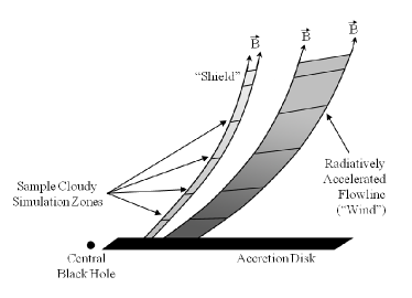
Figure 1: Schematic diagram of the structure of the radiatively accelerated magneto-centrifugal wind model (Everett, 2005). The sub parsec-scale accretion disk is the source of the continuum illuminating the wind. The wind has two distinct components. The leftmost, thinner component is the “shielding gas,” and is modeled as a pure magneto-centrifugal wind. The wider streamline on the right is the dusty wind which is propelled by both magneto-centrifugal and radiative acceleration. The black lines within the shield and streamline are examples of the zones in which Cloudy determines opacities and simulates photo-ionization. In our calculations, the shielding gas is set to have an effectively negligible column density so that the wind is dominated by the radiatively accelerated component.

In more detail, the program starts by calculating the pure magneto-centrifugal wind dynamics (see Figure 1; Everett 2005) without including the effects of radiation pressure. Parameters such as the black hole mass, column density at the base of the wind and starting location of the wind are specified here. In this phase, an estimation of the density and velocity structure of the wind as a function of height is calculated by a relatively simple semi-analytic model of the magneto-centrifugal acceleration of gas along a streamline (this is described in detail in Everett 2005). Next, Cloudy (Ferland et al., 1998) is used to calculate the photo-ionization of the gas and determine opacities throughout the structure of the wind, given the central continuum. With all of this information, the radiation pressure on the wind is calculated. This is exactly as described in Everett (2005), except for the addition of the opacity of dust, which is supplied via Cloudy’s “ISM” dust model. This information is passed back into the first step, where the MHD wind structure is modified accordingly. This process is iterated until convergence, which typically takes seven iterations.

Shown in Figure 2 are the gas streamlines for our fiducial model (with parameters as specified in § 4), plotted in the $z$ direction along the axis of symmetry as a function of the radial ($r$) direction. The streamlines are shown for each iteration of the MHD radiative wind code. The radiation pressure acts to bend the streamlines radially outward, away from the central source, with each iteration, until the code converges.

The second stage of our calculation uses the Monte Carlo simulation program MC3D (Wolf, 2003) to predict spectral energy distributions. The input for the simulation is the output from the MHD radiative wind code, which includes the structure of the wind and the SED of the central continuum source (we use the composite SED from Richards et al. 2006, modified to remove IR emission; see Fig. 3 and § 3.3 for more details). This input is passed to MC3D: this is a general purpose, 3D Monte Carlo code which calculates heating and emission when given a central radiative source surrounded by a scattering and absorbing medium. MC3D first determines the temperature of the dust grains due to heating from the continuum and reemission from other dust grains. In a second step, MC3D’s ray-tracer is then used to create the SEDs from 0.1 – 2000 ${\,\mu\rm m}$, which we plot from 2 – 100 ${\,\mu\rm m}$.

3 Methodology

Initial tests for basic functionality, stability and consistency of the code are documented in detail in Everett (2005). For this work, the code was compiled on a number of different machines and it was verified that identical results were produced on each machine. With confidence that the code performs as expected, we then investigated ways to minimize computation time while maintaining an acceptable level of accuracy. The bulk of the computing time is spent on generating the IR SED, and thus we analyzed the MC3D input parameters to determine both whether we could make our simulations more accurate without a significant increase in time, and whether the process could be sped up significantly without a loss of accuracy. These tests are reviewed in § 3.1

After these basic considerations, we set out to explore the physical parameter space that the model allows. AGNs exhibit a large range of observed parameters, with varying luminosities, central continuum shapes, central black hole masses, etc., and the way these parameters interact in producing an IR SED is not necessarily simple or obvious. Salient parameters were identified and tested against one another in order to determine their effects on the dusty wind, and therefore on the shape and power of the IR SED. An in-depth description of each parameter examined can be found in § 3.2 to § 4.

3.1 MC3D Testing Parameters

MC3D is a versatile code, with a range of customizable user-set parameters for modelling dust-temperature distributions and SEDs. We tested a number of these in order to determine an appropriate set of base parameters which maintain a reasonable degree of accuracy while minimizing the amount of time needed to generate the models.

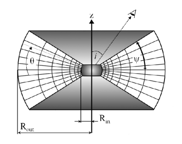
Figure 4: MC3D model geometry. Listed in Wolf (2003) as geometry 2D(b), it is a fully two-dimensional model, with vertical and radial dependences for the density distributions. The model is axisymmetric about the $z$ axis. Shown are the MC3D grid divisions in the $\theta$ and $r$ directions. The half-opening angle, $\psi$, is measured from the horizontal. The model radius is defined by $R_{out}$. The inclination angle, $i$, is defined from the normal, such that $i=90^{\circ}$ is perpendicular to the axis of symmetry.

MC3D has a number of model geometry options to choose from; because our model is axisymmetric, we utilized the fully two-dimensional model with a radial and vertical dependence for the density distribution (see Figure 4). Our default base values for testing the effects of varying these parameters were as follows: a maximum model radius, R_out, of 20 parsecs, with 30 sub-divisions (grid points) in the radial direction and 101 sub-divisions in the $\theta$ direction, a half-opening angle, $\psi$, of 75 degrees, and 100 photon packets per wavelength. We will discuss in more detail, below, our tests of these parameter settings; for all of the parameter changes discussed, Figure 5 displays the differences in the SED and Table 1 details the effects on the emission at 2, 3, 6, 10, and 50 ${\,\mu\rm m}$ as compared to the default parameters.

For example, decreasing the number of photon packets per wavelength from the default of 100 to 10 (Wolf, 2003) had little effect on the SED, but decreased the time required to compute the temperature distribution by almost a factor of five. The variation that is seen between SEDs generated with 10 or 100 photon packets per wavelength is a minor loss of accuracy in the emission from the hottest dust; the greatest difference is at $2{\,\mu\rm m}$, where the model with 10 photon packets shows 1.61 times the emission as the model with 100 photon packets. As this loss is not relevant for our purposes – the largest discrepancy is seen at wavelengths $\lesssim$ 3 ${\,\mu\rm m}$ where the accretion disk and host galaxy typically contribute significantly to the observed emission – and the increase in computation efficiency is great, we opted to use 10 photon packets per wavelength for all of our simulations.

Increasing the resolution of the grid by choosing 201 $\theta$ subdivisions increased the computation time for the SED by several hours, with little benefit. Again, the largest difference is seen at $2{\,\mu\rm m}$, where the test model with 201 $\theta$ subdivisions showed 1.11 times the emission compared to the default of 101 $\theta$ subdivisions.

Decreasing R_out to 10 parsecs had little effect on the time for generating the temperature distribution, but increased the time for generating SEDs by more than a factor of 3. The difference in the SEDs is slight. The greatest difference is seen at long wavelengths; at $50{\,\mu\rm m}$, the test model with R_out = 10 pc displays 0.88 times the emission compared to the default model with R_out = 20 pc. We retain the value of 20 pc for R_out.

Decreasing the half-opening angle from $\psi=75^{\circ}$ to $\psi=60^{\circ}$ also served to increase, rather than decrease, the computation time. The SED showed a very slight overall change in normalization, with the model with $\psi=60^{\circ}$ showing a minor decrease in emission.

To summarize, for the rest of our models, we take the MC3D parameters as: 10 photon packets per wavelength, 101 $\theta$ sub-divisions, R_out = 20 pc, and $\psi=75^{\circ}$.

A full list of these parameters, the range of values explored, and the corresponding times to generate a temperature distribution and SED can be found in Table 2. Most of the computations were done on a workstation with a dual-core CPU, each at 3.16 GHz and a workstation with a quad-core CPU, each at 2.83 GHz.

3.2 Exploring the Parameter Space

Turning to more physical parameters, we have investigated variations in the final IR SED due to inclination angle of the observer ($i$), the base column density of the wind ($N_{H,0}$), and changes to the central continuum shape, luminosity, and black hole mass. All parameter changes are specified before the wind structure is calculated, with the exception of the inclination angle, which is only specified when MC3D is called. We chose to run many of our models at an inclination of $i=60^{\circ}$, as choosing inclination angles smaller than that tended to increase the computation time. Table 3 details these parameters along with corresponding relevant information, such as the terminal velocity of the wind and the mass outflow rate, as calculated by the MHD wind model, as well as the kinetic luminosity of the outflows.

The relative power and shape of the SED were only slightly affected by a change in the inclination angle, with larger inclination angles showing a slightly lower normalization in the overall IR SED (see Figures 6 and  7). This indicates that the IR emission is consistent with being optically thin at most wavelengths of interest.

The integrated luminosity varied significantly with changes in the column density, with higher columns producing a higher overall infrared luminosity. We chose to maintain a fixed column density $N_{H,0}=10^{25}$ cm^-2 for the remaining models, as this was the only column which could match the order of magnitude of luminosity comparable to a typical quasar ($L\approx 10^{45}$ erg s^-1). Such a model generates mass outflow rates on order of $1{\rm\,M_{\odot}}$ yr^-1 (see Table 3).

3.3 The Central Continuum

In order to investigate what sort of radiative output we would expect to see from the dusty wind, we specify a central input continuum that represents an approximation of the emission from the accretion disk around the black hole. We used a composite created from broadband photometry of 259 optically luminous Sloan Digital Sky Survey (SDSS) quasars, as described by Richards et al. (2006), as a starting point for this central continuum (see Figure 8 for a plot of this continuum, as well as the input continua modified from it). The optical and UV portions of the spectrum are assumed to be a fair representation of the emission from the accretion disk. However, the observed “IR hump” (from 1 ${\,\mu\rm m}$ – 100 ${\,\mu\rm m}$) in this composite spectrum is due to the dust emission that we aim to model. Therefore, the IR hump was removed and replaced with a simple power law extrapolated from the optical continuum. Though the observed IR hump from 1 – 100 ${\,\mu\rm m}$ is quite prominent, common features such as the 10 and 18 ${\,\mu\rm m}$ silicate emission features are not apparent, due to a lack of spectral resolution in the broad-band photometry and the effect of smearing out such features with composite averaging. Nevertheless, such a composite SED serves as an excellent basis for comparing to our IR SEDs models, as a check to ensure that the power and general shape can be matched. We will be testing whether the wind model can account for the empirical IR hump.

3.3.1 Changes to the Central Continuum: $\alpha_{ox}$

The spectral index $\alpha_{ox}$ describes the amount of energy emitted in the X-ray relative to the amount emitted in the UV/optical, and can be considered a measure of the “X-ray brightness” of a source. The parameter is defined as follows (Tananbaum et al., 1979):

$$\alpha_{ox}=-0.384\mathrm{\;log}\left[\frac{L_{\nu}(2~{}\mathrm{keV})}{L_{\nu}(2500~{}\mathrm{\AA})}\right]$$ (1)

Quasars have been found with a range of $\alpha_{ox}$ values, typically varying from 1.2 to 1.8. There is an anti-correlation between $\alpha_{ox}$ and UV luminosity, as more luminous AGNs show less X-ray emission relative to emission in the optical wavelengths (e.g., Just et al., 2007; Steffen et al., 2006). In order to test this range of $\alpha_{ox}$ values, we selected an “average” value of 1.6 (appropriate for the UV luminosity of our fiducial model), and then modified the input continuum (see Figure 3) to reflect extreme values of $\alpha_{ox}=1.1$ (much higher than average output in the X-ray), and $\alpha_{ox}=2.1$ (much lower than average output in the X-ray). The X-ray modification begins at $7\times 10^{16}$ Hz and extends to $10^{19}$ Hz. The discontinuity at $\nu=7\times 10^{16}$ Hz is not physical, but serves to isolate the effect of the X-ray continuum from that of the far-UV.

These new continua are passed as parameters to the wind and radiative acceleration code. The results of these changes are described in § 4.

3.3.2 Changes to the Central Continuum: $L/L_{Edd}$

Initial tests of the wind model were performed with an Eddington ratio of $L/L_{Edd}=0.01$. Such an Eddington ratio is characteristic of the Seyfert regime, but may not accurately describe quasar luminosities. In order to test the model at the higher luminosities more appropriate to quasars, we incrementally increased the Eddington ratio to $L/L_{Edd}=0.1$ by increasing the total luminosity and keeping $M_{BH}$ fixed. Furthermore, we tested the effects of changing black hole mass, which has the effect of changing the Eddington luminosity, since:

$$L_{Edd}=1.25\times 10^{38}\left[\frac{M}{{\rm\,M_{\odot}}}\right]\mathrm{erg\;s}^{-1}$$ (2)

We tested masses ranging from $M_{BH}=10^{8}-10^{9}\mathrm{{\rm\,M_{\odot}}}$. We note that although the part of the code that generates the wind structure was able to accommodate such high luminosities with relative ease, the time for generating the final SED increased by a factor of three or more at higher luminosities.

4 Results

As a basis of comparison for many of our results, we adopt a fiducial model with the following parameters: $N_{H,0}=10^{25}$ cm^-2, $L/L_{Edd}=0.1$, $M_{BH}$ = 10${}^{8}{\rm\,M_{\odot}}$, $i=60^{\circ}$, and $\alpha_{ox}=1.6$. The Eddington luminosity for a black hole of mass $M_{BH}$ = 10${}^{8}{\rm\,M_{\odot}}$ is $1.25\times 10^{46}$ erg s^-1, giving a luminosity at 5100 Å of $L_{5100}=3.7\times 10^{29}$ erg s^-1 Hz^-1 for an Eddington ratio of $L/L_{Edd}=0.1$. Figure 8 shows this fiducial model, plotted with the input continuum, and the original Richards et al. (2006) composite SED. The sum of the predicted IR SED and the input SED is also displayed. The composite SED is normalized to the input SED at $L_{5100}$, and the output SED has been integrated over $4\pi$ steradians to match the units of the observations.

With the base column density of $N_{H,0}=10^{25}$ cm^-2, the predictions approximately match the power expected from the Richards et al. (2006) composite SED. The observed composite SED has $\simeq 82\%$ as much power radiated in the IR (from $2-100{\,\mu\rm m}$) as in the optical/UV (from $2{\,\mu\rm m}-1000$ Å)̇ When normalized at $L_{5100}$, our model with the smaller column density of $N_{H,0}=10^{24}$ cm^-2, $L/L_{Edd}=0.01$, $M_{BH}$ = 10${}^{8}{\rm\,M_{\odot}}$, $i=60^{\circ}$, and $\alpha_{ox}=1.6$ has only 45% as much power radiated in the IR as in the composite optical/UV, which does not match the expected output. Our model with a higher column of $N_{H,0}=10^{25}$ cm^-2 (and all other parameters as before) radiates 97% as much power in the IR as in the composite optical/UV, which is more than what is expected. Our fiducial model, with a higher column of $N_{H,0}=10^{25}$ cm^-2 and a higher Eddington ratio of $L/L_{Edd}=0.1$, has $\simeq 70\%$ as much power radiated in the IR as in the composite optical/UV, which is closer to the expected 82%.

While the model SEDs can account for the gross power and shape of the composite SED with the parameter values in the fiducial model, there are specific features that do not match. Specifically, the composite has more power at both shorter (2–8 µm) and longer ($>30$ µm) wavelengths, and the fiducial model SEDs show more prominent and sharply peaked silicate features at both 10 and 18 µm. On this second point, note that the composite by construction smears out spectral structure such as the silicate emission bumps as it is made using broad-band photometry; many mid-IR spectra of luminous quasars, however, show prominent silicate emission features (see, e.g., Siebenmorgen et al., 2005; Hao et al., 2007; Netzer et al., 2007; Mason et al., 2009; Deo et al., 2011). We also note that at long wavelengths, we do not expect much of an AGN contribution from the dusty wind. Empirically, far-infrared emission of AGNs is typically weak unless the host is actively star-forming (Schweitzer et al., 2006; Netzer et al., 2007). In fact, the composite SED contains little data beyond 24 ${\,\mu\rm m}$, with that part of the SED constructed by “gap repair,” replacing the missing data with information extrapolated from Elvis et al. (1994) who used IRAS photometry of low redshift quasars at these wavelengths. We explore these issues in more detail in § 5.

4.1 Mass outflows, terminal velocities, and kinetic luminosities

Table 3 contains information on the mass outflow rates ($dM/dt$), terminal velocities ($v_{term}$), and kinetic luminosities ($L_{kin}$) of each of the models. We see mass outflow rates ranging from $0.96-4.19{\rm\,M_{\odot}}$ yr^-1, terminal velocities ranging from $1904-7992$ km sec^-1, and kinetic luminosities ranging from $1.13\times 10^{42}-7.71\times 10^{43}$ erg s^-1. These values are strongly affected by the black hole mass of the model: the largest mass outflows, terminal velocities, and kinetic luminosities are produced by the models with the highest black hole masses, even at lower Eddington ratios.

4.2 Results of varying inclination angle

Here, we examine the result of varying the inclination angle from $i=90^{\circ}$ (edge-on) to $i=30^{\circ}$ (nearly face-on). Inclination angles smaller than $i=30^{\circ}$ were not considered because of the great increase in time required to compute the SEDs. As the first phase of our parameter exploration, these models were run at luminosities $L/L_{Edd}=0.01$ and $0.03$, lower than that of our fiducial model.

Figure 6 shows the result of varying the inclination angle for a model with $N_{H,0}=10^{24}$ cm^-2, $L/L_{Edd}=0.01$, $M_{BH}$ = 10${}^{8}{\rm\,M_{\odot}}$, and $\alpha_{ox}=1.6$. This model is different from our fiducial model in two ways: it has both a lower column density ($N_{H,0}=10^{24}$ cm^-2, as compared to $N_{H,0}=10^{25}$ cm^-2), and a lower Eddington ratio ($L/L_{Edd}=0.01$, as compared to $L/L_{Edd}=0.1$). Table 4 details the amount of power emitted in the IR as compared to the optical/UV for each model, as well as the ratios of emission at 3, 6, 10, and 50 ${\,\mu\rm m}$, relative to the $i=90^{\circ}$ model. Varying the inclination angle for these parameters has almost no effect on the shape or normalization of the SEDs. The lack of variation indicates that IR emission must be optically thin at the wavelengths of interest.

However, when we move to a higher base column density, variations in the SED start to become apparent. Figure 7 shows the effects of inclination angle for a model with $N_{H,0}=10^{25}$ cm^-2, $L/L_{Edd}=0.01$, $M_{BH}$ = 10${}^{8}{\rm\,M_{\odot}}$, and $\alpha_{ox}=1.6$. This model is different from our fiducial model as it has a lower Eddington ratio ($L/L_{Edd}=0.01$, compared to $L/L_{Edd}=0.1$). Variations in the SED are much more apparent than they were at the lower column density of $N_{H,0}=10^{24}$ cm^-2. Table 5 details the amount of power emitted in the IR as compared to the optical/UV for each model, as well as the ratios of emission at 3, 6, 10, and 50 ${\,\mu\rm m}$, relative to the $i=90^{\circ}$ model.

At wavelengths $>5{\,\mu\rm m}$, the effect of decreasing the inclination angle is primarily a change in normalization, with smaller inclination angles (more face-on lines of sight) displaying more power. At wavelengths $<5{\,\mu\rm m}$, the effect is more pronounced, and the SEDs display a change in shape as well as normalization, with larger inclinations (more edge-on lines of sight) showing a marked decrease in the amount of emission from the hottest dust. At $3{\,\mu\rm m}$, the $i=30^{\circ}$ SED displays 2.4 times more emission than the $i=90^{\circ}$ SED, and 1.48 times more emission at $50{\,\mu\rm m}$. The results of varying inclination angle are similar when looking at the model with a slightly higher Eddington ratio, $L/L_{Edd}=0.03$, which is still smaller than that of our fiducial model.

The measurable variation at higher column densities indicates that the wind is becoming more optically thick — especially at the shortest wavelengths — as the column increases.

4.3 Results of varying $\alpha_{ox}$

Next, we examine the effects of changing the amount of energy emitted in the X-ray relative to the amount emitted in the UV/optical, defined by parameter $\alpha_{ox}$. Figure 9 displays the results of varying $\alpha_{ox}$ as compared to our fiducial model, with $N_{H,0}=10^{25}$ cm^-2, $L/L_{Edd}=0.1$, $M_{BH}$ = 10${}^{8}{\rm\,M_{\odot}}$, and $i=60^{\circ}$. For reference, a $\Delta\alpha_{\rm ox}$ value of 1.0 corresponds to a factor of $\approx 400$ difference in X-ray luminosity at 2 keV for a set value of $L_{2500~{}\AA}$. The depressed X-ray emission of the X-ray faint model crudely mimics the effect of strong X-ray absorption seen in some broad absorption line quasars (e.g., Gallagher et al., 2006). The X-ray bright model with $\alpha_{ox}=1.1$ displays the highest overall luminosity at wavelengths $>4{\,\mu\rm m}$, with emission that decreases at wavelengths $<4{\,\mu\rm m}$, relative to the other models. Our fiducial model, with $\alpha_{ox}=1.6$, shows somewhat lower emission than both the X-ray bright and X-ray faint models.

Table 6 shows the amount of power emitted in the IR as compared to the optical/UV for each model, as well as the ratios of emission at 3, 6, 10, and 50 ${\,\mu\rm m}$, relative to the $\alpha_{ox}=1.6$ fiducial model. When the Richards et al. (2006) composite is normalized to the $L_{5100}$ value of the input continuum, the fiducial model displays 69.7% as much power in the IR as compared to the optical/UV power in the Richards et al. (2006) composite SED. The $\alpha_{ox}=1.1$ and $\alpha_{ox}=2.1$ models display 102% and 84.9% as much power in the IR as compared to the composite optical/UV, respectively.

The X-ray faint model with $\alpha_{ox}=2.1$ displays more emission at shorter wavelengths ($<4{\,\mu\rm m}$) than either of the other models, and at wavelengths $>4{\,\mu\rm m}$ shows a change in normalization compared to the other models. At wavelengths $>50{\,\mu\rm m}$, the SEDs for all the models appear to converge. Compared to the fiducial model with $\alpha_{ox}=1.6$, the greatest difference is seen for the $\alpha_{ox}=1.1$ model which shows 1.55 times more emission at $6{\,\mu\rm m}$.

These results are perhaps counterintuitive, and reveal the complex role of the SED in both accelerating and heating the dust. The X-ray bright model has significantly more power available to illuminate the dusty medium, and therefore it makes sense that the IR SED is more luminous relative to the other two models. However, the relative lack of emission at the shortest wavelengths in the X-ray bright model indicates that there is a smaller volume of dust at the highest temperatures, a natural consequence of a wind that is more radially “combed out” (and hence has a narrower wedge of material near the sublimation temperature).

In addition, the dust sublimation radius, $R_{\rm sub}$, is $\sim 13\%$ larger for the $\alpha_{\rm ox}$=1.1 models relative to the $\alpha_{\rm ox}$=1.6 models (see Table 9). We consider the 2% difference in sublimation radii between the $\alpha_{\rm ox}$=1.6 and 2.1 runs to be the same, within the precision of the simulation.

These changes highlight the complex nature of how enhanced X-ray emission impacts winds. First, while X-rays contribute to heating, their efficiency is quite low compared to UV photons: at 300 eV (near the $\alpha_{\rm ox}$ jumps), the dust opacity (scattering plus absorption) is about an order of magnitude below the UV opacity (see Fig. 9 in Draine 2003). Therefore, it requires a strong increase in the X-ray flux to yield, e.g., a factor of two increase in the near-IR flux. A second effect is the increased momentum transfer per photon of X-rays vs. UV light: X-rays are both more likely to scatter (versus being absorbed) and carry more momentum. Supporting this interpretation, the X-ray-faint model with $\alpha_{\rm ox}=2.1$ shows the strongest short ($\lesssim 4$ µm) wavelength emission. The UV power provides a “floor” to $R_{\rm sub}$; the smaller X-ray power in the $\alpha_{\rm ox}=2.1$ model does not change the sublimation radius significantly relative to the $\alpha_{\rm ox}=1.6$ model, while increasing the relative X-ray power by setting $\alpha_{\rm ox}=1.1$ preferentially pushes out $R_{\rm sub}$ and accelerates the wind more rapidly. Both effects reduce the volume of dust heated to the highest temperatures, and thus the relative power coming out at the shortest IR wavelengths.

Figure 10 displays the results of varying $\alpha_{ox}$ for a model with $N_{H,0}=10^{25}$ cm^-2, $L/L_{Edd}=0.01$, $M_{BH}$ = $5\times 10^{8}{\rm\,M_{\odot}}$, and $i=60^{\circ}$. This model has a lower Eddington ratio than our fiducial model, as well as a higher black hole mass. The X-ray bright model with $\alpha_{ox}=1.1$ displays the highest overall luminosity. The model with $\alpha_{ox}=1.6$ shows a change in normalization, with less emission than the $\alpha_{ox}=1.1$ model, and little effect on the SED shape. Table 7 shows the amount of power emitted in the IR as compared to the optical/UV for each model, as well as the ratio of emission at 3, 6, 10, and 50 ${\,\mu\rm m}$, relative to the $\alpha_{ox}=1.6$ model. When the Richards et al. (2006) composite is normalized to the $L_{5100}$ value of the input continuum, the model with $\alpha_{ox}=1.6$ displays about 80% as much power in the IR as compared to the optical/UV power in the Richards et al. (2006) composite SED. The $\alpha_{ox}=1.1$ and $\alpha_{ox}=2.1$ models display $\sim 120$% and $\sim 90$% as much power in the IR as compared to the composite optical/UV, respectively.

The X-ray faint model with $\alpha_{ox}=2.1$ also shows a change in normalization compared to the X-ray bright model, with less overall emission, and is very similar to the model with $\alpha_{ox}=1.6$, though it displays a slight increase in emission at wavelengths $<8{\,\mu\rm m}$. Compared to the model with $\alpha_{ox}=1.6$, the $\alpha_{ox}=1.1$ model shows 1.75 times more emission at $3{\,\mu\rm m}$ and 1.27 times more emission at $50{\,\mu\rm m}$, and the $\alpha_{ox}=2.1$ model shows only 1.20 times more emission at $3{\,\mu\rm m}$ and displays the same amount of emission at $50{\,\mu\rm m}$. As in the previous set of models, the impact of changing $\alpha_{\rm ox}$ from 1.6 to 1.1 is to push out $R_{\rm sub}$ by $\sim 18\%$; the difference between the two X-ray fainter models of 2% is not considered significant.

The difference in the wind response to varying $\alpha_{ox}$ models when the values of $M_{BH}$ and $L/L_{Edd}$ are also changed illustrates the interplay between these parameters, and the challenges in isolating the effects of the SED. An increase in $M_{BH}$ of a factor of 5 coupled with a decrease in $L/L_{Edd}$ of a factor of 10 means that the luminosity is a factor of 2 fainter than in the previous model described in this section. A lower luminosity coupled with a larger black hole mass generates a wind with more vertical streamlines, because the net radial component of the ejection (centrifugal plus radiative minus gravitational) force will be reduced. For example, in the $L/L_{\rm Edd}=0.1$ X-ray bright model, the wind streamlines at large radii have an angle from the disk of $63^{\circ}$ vs. $74^{\circ}$ for the lower luminosity, X-ray bright model. The more vertical wind structure of the lower luminosity models keeps the dusty wind closer to the illuminating source for longer, but apparently decreases the observed emission from the hottest dust. We consider it likely that this is an artifact of the observer’s inclination angle (see Figure 7); the more vertical (because of lower radial acceleration) wind will be more optically thick at shorter wavelengths. The view of the hottest dust is therefore obscured for an observer viewing angle of 60^∘.

4.4 Result of varying the black hole mass

We examine the effects of changing the mass of the central black hole, with values from $M_{BH}$ = $10^{8}-10^{9}{\rm\,M_{\odot}}$. Altering $M_{BH}$ also changes the Eddington luminosity (see Equation 2). For $M_{BH}$ = $10^{8}{\rm\,M_{\odot}}$, the Eddington luminosity is $L_{Edd}=1.25\times 10^{46}$ erg s^-1, which gives a luminosity at 5100 Å of $L_{5100}=3.7\times 10^{28}$ erg s^-1 Hz^-1 for $L/L_{Edd}=0.01$. The luminosities scale linearly with the black hole mass. In these tests, we keep $L/L_{Edd}=0.01$ fixed.

Figure 11 shows the effect of changing the black hole mass, which changes the luminosity for a fixed $L/L_{Edd}$. In this situation, higher black hole masses produce overall more luminous SEDs. For both $M_{BH}$ = $5\times 10^{8}{\rm\,M_{\odot}}$ and $M_{BH}$ = $10^{9}{\rm\,M_{\odot}}$, the shape and normalization of the SED is affected from $2-40{\,\mu\rm m}$ as compared to the $M_{BH}$ = $10^{8}{\rm\,M_{\odot}}$ model. Table 8 shows the amount of power emitted in the IR as compared to the optical/UV for each model, as well as the ratios of emission at 3, 6, 10, and 50 ${\,\mu\rm m}$, relative to $M_{BH}$ = 10${}^{8}{\rm\,M_{\odot}}$. The higher $M_{BH}$ models show a more peaked SED shape from $3-30{\,\mu\rm m}$ as compared to the $M_{BH}$ = $10^{8}{\rm\,M_{\odot}}$ model, as well as the overall increase in luminosity. Compared to the model with $M_{BH}$ = $10^{8}{\rm\,M_{\odot}}$, the model with $M_{BH}$ = $5\times 10^{8}{\rm\,M_{\odot}}$ displays $\sim 60$ times the emission at $10{\,\mu\rm m}$ and $\sim 80$ times the emission at $50{\,\mu\rm m}$, whereas the model with $M_{BH}$ = $10^{9}{\rm\,M_{\odot}}$ displays $\sim 130$ times the emission at $10{\,\mu\rm m}$, and $\sim 40$ times the emission at $50{\,\mu\rm m}$. Given that the emission at these comparison wavelengths is not just scaling linearly with the luminosity (which is increasing by a factor of 5 and 10 as $M_{BH}$ is increased by the same factors), the change in black hole mass clearly has a direct influence on the IR power.

4.5 Result of varying $L/L_{Edd}$

We examine the effects of changing the Eddington ratio, $L/L_{Edd}$, which, for a given black hole mass, has the effect of changing the bolometric luminosity. For $M_{BH}=10^{8}{\rm\,M_{\odot}}$, an $L/L_{Edd}$ ratio of 0.1 gives a luminosity at 5100 Å of $L_{5100}=3.7\times 10^{29}$ erg s^-1 Hz^-1; $L/L_{Edd}=0.07$ gives $L_{5100}=2.6\times 10^{29}$ erg s^-1 Hz^-1; $L/L_{Edd}=0.03$ gives $L_{5100}=1.1\times 10^{29}$ erg s^-1 Hz^-1; and an $L/L_{Edd}=0.01$ gives $L_{5100}=3.7\times 10^{28}$ erg s^-1 Hz^-1.

Figure 12 displays the effects of varying $L/L_{Edd}$ (changing the luminosity). As is expected, higher $L/L_{Edd}$ ratios display a greater luminosity as compared to lower $L/L_{Edd}$ ratios. The $L/L_{Edd}=0.1$ and $0.07$ models are very similar in shape, differing only by a normalization factor. The $L/L_{Edd}=0.03$ and $0.01$ models show a marked change in SED shape as compared to the higher luminosity models, in addition to displaying a lower overall luminosity. Table 9 shows the amount of power emitted in the IR as compared to the optical/UV for each model, as well as the ratios of emission at 3, 6, 10, and 50 ${\,\mu\rm m}$, relative to $L/L_{Edd}=0.1$. As compared to the fiducial model with $L/L_{Edd}=0.1$, the $L/L_{Edd}=0.07$ model displays around 0.8 times the emission at each wavelength examined, whereas the $L/L_{Edd}=0.03$ model displays $\sim 0.4$ times the emission at $3{\,\mu\rm m}$ and 0.5 times the emission at $50{\,\mu\rm m}$.

4.6 Distinguishing between $M_{BH}$ effects and $L/L_{Edd}$ effects

As changing both $M_{BH}$ and $L/L_{Edd}$ effectively results in a change in luminosity, one might ask whether the changes to these parameters are redundant. To isolate these effects, we plot two models with the same input luminosity, $L_{5100}=3.7\times 10^{29}$ erg s^-1 Hz^-1 (see Figure 13). The two plots are very similar, but not identical: the model with a higher black hole mass and lower Eddington ratio displays a higher normalization from $2-40{\,\mu\rm m}$. These results suggest that the properties are not redundant, though running further models for comparison would be of great benefit.

5 Conclusions and Discussion

We have investigated the parameter space of our model of the torus as a dusty magneto-centrifugal wind with radiative acceleration. We have examined a number of interesting and important parameters and illustrated how they affect the IR SED of an AGN. We have verified that with input SEDs of bolometric luminosities $L\approx 10^{44}-10^{46}$ erg s^-1 and a base column density of $10^{25}$ cm^-1, the code produced reasonable IR SEDs with approximately the right shape and luminosity ($L\approx 10^{43}-10^{45}$ erg s^-1) as expected from the Richards et al. (2006) composite of optically luminous SDSS quasars. This is a promising result for a relatively simple model given that we have not attempted any fitting. A benefit to our model is that we are able to see directly the effects of various physical parameters on the final IR SED, which ultimately will allow us to understand the physical properties of the torus itself. By determining which physical parameters have an observable effect on the IR SEDs, and narrowing down these parameters to ascertain which ones allow us to generally reproduce the power expected, we have established a reasonable starting point from which we can expand and further refine our model.

We summarize our results as follows:

1. Varying the inclination angle has little effect at base column densities $\leq 10^{24}$ cm^-2, but becomes more pronounced at base column densities $\geq 10^{25}$ cm^-2. This indicates that the emission is becoming slightly more optically thick as the column increases. The most salient difference (see Fig. 8) is a deficit at the shortest wavelengths for the larger inclination angles, indicating that emission from the hottest dust, at the smallest radii, is being blocked.

2. The parameter $\alpha_{ox}$, characterizing the amount of energy emitted in the X-ray relative to the amount emitted in the optical/UV, has slight but measurable effects on the IR SEDs. The X-ray bright model, with $\alpha_{ox}=1.1$, displays the highest overall luminosity, with emission that decreases at wavelengths $<4{\,\mu\rm m}$. Both the X-ray bright ($\alpha_{ox}=1.1$) and X-ray faint ($\alpha_{ox}=2.1$) models display marginally more emission than the fiducial model with $\alpha_{ox}=1.6$.

3. The short wavelength ($<5$ µm) emission appears to be sensitive to the relative power of X-rays relative to UV in the SED, offering promise for using the properties of the IR SED to constrain the strength and shape of the high energy continuum. This illustrates the utility of models where the IR-emitting medium can respond dynamically to the input SED; in static models the incident spectrum is quickly thermalized and information on its shape is lost.

4. Higher black hole masses produce more luminous IR SEDs, for a fixed value of $L/L_{Edd}$. The SEDs for $M_{BH}\geq 5\times 10^{8}{\rm\,M_{\odot}}$ are more peaked from $\sim 3-30{\,\mu\rm m}$ as compared to the SEDs for $M_{BH}<5\times 10^{8}{\rm\,M_{\odot}}$.

5. Higher Eddington ratios produce more luminous IR SEDs. The SEDs for $L/L_{Edd}\geq 0.03$ are more peaked from $\sim 3-30{\,\mu\rm m}$ as compared to SEDs for $L/L_{Edd}<0.03$.

6. Although changes to both $L/L_{Edd}$ and $M_{BH}$ are effectively changes to the overall input luminosity, these effects may not be redundant, and appear to be slightly distinguishable from each other. The model with a higher black hole mass and lower Eddington ratio displays a higher normalization from $2-40{\,\mu\rm m}$.

At present, although our model is producing approximately the right amount of power, it does not adequately reproduce the amount of expected emission in the hot dust, at wavelengths $\lesssim 8{\,\mu\rm m}$. This may be due in part to inclination angle effects. As discussed in § 4.2, although inclination angle has little effect at lower column densities, it begins to show an effect at column densities of $N_{H,0}=10^{25}$ cm^-2, with smaller inclination angles displaying more power, particularly at wavelengths $<5{\,\mu\rm m}$. It is possible that this effect is amplified not only by an increase in column density, but by an increase in luminosity as well. We chose an inclination angle of $i=60^{\circ}$ for the majority of our models in order to increase our computational efficiency, which allowed us to run more models in a shorter period of time. However, such an inclination angle is not likely to represent the average for Type 1 objects; a more characteristic choice would have been between $i=45^{\circ}$ and $i=30^{\circ}$. The choice of $i=60^{\circ}$ means that we may be obscuring the innermost parts of the wind, and therefore missing the hottest dust, in many of our models.

Another possibility is that our assumption of an ISM dust composition is not entirely correct. We assume a single silicate dust sublimation radius, which neglects the hot graphite grains that can exist at smaller radii, and thus we are missing that emission. Further investigations into the details of our dust composition and sublimation radius are therefore required. Changing grain composition can also affect the profile of the silicate features.

The above simulations with MC3D required long run-times. The fiducial model takes $\sim$3–4 days on a 4-core desktop machine to construct an SED for a single viewing/inclination angle. Further, smaller sublimation radii and smaller inclination angles require much longer run-times. For example, our fiducial model with a modified $R_{\rm sub}=1.5675\times 10^{18}~{}{\rm cm}$ requires $\sim$2–3 months on an 8-core desktop machine. Smaller sublimation radii translate to higher grid resolutions in the grid setup procedure for MC3D. To explore the sensitivity of our results to the effects of a smaller sublimation radius, we found it necessary to port MC3D to run on the many-core symmetric multi-processing (SMP) compute nodes of SHARCNET. The fiducial model now takes $\sim 19$ hours when using 32 nodes; the highest resolution run mentioned above takes slightly longer than a week.

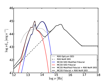
Figure 14: The fiducial model with a smaller dust-sublimation radius shows an SED (blue solid line) peaking in the near-IR. As the dust-sublimation radius is increased the SED power decreases progressively in the near-IR and the peak emission shifts to longer wavelengths.

We modified our fiducial model, setting the inner radius of the dusty wind to be $1.5675\times 10^{18}~{}{\rm cm}$, about half that of the original fiducial model, keeping all other parameters fixed. A maximum temperature of 1615 K was reached within the dusty wind as modeled by MC3D, as opposed to approximately 800–1200 K in previous variations of the fiducial model. This model reproduces the blackbody-like shape of the near-IR emission between 1–8 µm (see Figure 14) that is seen in mid-IR spectra of luminous quasars (e.g., Netzer et al., 2007; Deo et al., 2011). The SED corresponding to our fiducial run (red curve) and the high-resolution run (blue curve), bracket the average near-IR emission in the composite SED of Richards et al. (2006). The composite mean SED is an average over several important parameters such as inclination, luminosity and $M_{BH}$, and for a more accurate comparison, one would have to average over the similar range of models. That full study is beyond the scope of this paper, but we find that, in our predicted SEDs, the near-IR hot-dust luminosity decreases as we increase the inclination angle, giving approximately the correct trend. These results show that changes in the dust sublimation radius approximate the expected presence of hot graphite grains, and corresponding grid resolution (an effect of the choice of grid construction process) are important effects to consider when comparing model SEDs to observations.

We have explored a wider parameter space of this model based originally on the hydro-magnetic wind model of Königl & Kartje (1994). Our results are roughly consistent with theirs, with our models displaying similar $10{\,\mu\rm m}$ micron emission to their model (labeled as ‘A2’ in Königl & Kartje 1994), with $M_{BH}=10^{7}{\rm\,M_{\odot}}$, a bolometric luminosity $L_{bol}=10^{45}$ erg s^-1, and a mass outflow rate of 1.0 ${\rm\,M_{\odot}}$ yr^-1. We do not, however, see the silicate feature in absorption, as they do with their model ‘A3’, with $M_{BH}=10^{7}{\rm\,M_{\odot}}$, a bolometric luminosity $L_{bol}=10^{44}$ erg s^-1, and a mass outflow rate of 3.0 ${\rm\,M_{\odot}}$ yr^-1, even in our models with extremely high mass outflow rates ($>4.0{\rm\,M_{\odot}}$ yr^-1) and overall higher mass. Nenkova et al. (2008b) also see the silicate feature in absorption with many of their clumpy tori models. This may in part mean that a higher resolution is required to resolve the wind, although models with a significantly increased resolution would also require an increase in computation time (see above discussion). Furthermore, Königl & Kartje (1994) add in radiative acceleration only approximately; it is possible that with more realistic radiative acceleration added in, the wind accelerates off the disk quickly enough that the density drops very quickly with height, and only a very small region at the disk surface remains where we might observe silicate absorption.

Curiously, we find that the shape of our SEDs, in general, are similar to Schartmann et al. (2008)’s clumpy, face-on models, and are rather dissimilar to their continuous models (see the upper left panel in Figure 10 of Schartmann et al. 2008). We assume that they take the same parameters as described in Schartmann et al. (2005): a black hole mass of $M_{BH}=6.6\times 10^{7}{\rm\,M_{\odot}}$, and an $L_{disk}/L_{Edd}$ value of 0.06, parameters which are descriptive of the lower luminosity Seyfert regime of AGNs. Although our models are geared more towards describing luminous quasars, their model is most comparable to our model with $M_{BH}=1\times 10^{8}{\rm\,M_{\odot}}$ and $L/L_{Edd}=0.07$. Again, however, we do not see the silicate feature in absorption as they do for edge-on models.

5.1 Future Work

Future work on this model will entail refining our parameters, such as testing smaller inclination angles to determine whether we can more accurately reproduce the emission from the hottest dust. Along these lines, we aim to decrease the computation time further, to enable us to resolve the inner graphite-dominated region that likely gives rise to the near-IR emission. Then, we will be able to explore the importance of multiple dust components, at the necessary higher resolution. Further next steps will involve detailed comparisons of the predicted SEDs with a broad sample of IR observations, for example from the Spitzer Space Telescope. Such in-depth comparisons will allow us to further constrain the salient parameters that we have isolated in this paper.

Currently, we are investigating the effects of increasing the “shielding gas” column density, $N_{sg}$. The high X-ray flux from the AGN is prone to over-ionizing the gas in the wind. A thick layer of hot, highly ionized “shielding gas,” located interior to the wind-launching dust sublimation radius, is required in order to prevent this over-ionization. Such a construct was first hypothesized in the context of continuous quasar winds as the “hitchhiking gas” described by Murray et al. (1995), and later studied by Proga & Kallman (2004) and Everett (2005). Subsequent empirical evidence for the shielding gas was found in the signatures of high column density X-ray absorption in broad absorption line quasars (e.g. Gallagher et al., 2006). Modifications to the MC3D code are required in order to deal with absorbed continua passing through different column densitities of shielding gas to determine the effect on the dust sublimation radius and output IR SED.

Finally, another step towards perhaps more realistic models would be to simulate dusty winds of a filamentary nature. Such a model may better represent the structures seen in interferometric observations of AGNS (see, e.g., Tristram et al., 2007).

Table 1: Variations in testing parameters for MC3D

Parameter Change	$2{\,\mu\rm m}$ Ratio	$3{\,\mu\rm m}$ Ratio	$6{\,\mu\rm m}$ Ratio	$10{\,\mu\rm m}$ Ratio	$50{\,\mu\rm m}$ Ratio
Default	1.00	1.00	1.00	1.00	1.00
10 photons/$\lambda$	1.61	1.14	0.99	0.99	0.98
201 $\theta$ divisions	1.11	1.04	1.00	0.99	1.00
$R_{out}=10$ pc	1.04	1.04	1.02	0.99	0.88
$\psi=60^{\circ}$	0.98	0.96	0.96	0.96	0.96

Note. — All models are compared to the model with default base parameters of 100 photon packets per wavelength, 101 $\theta$ sub-divisions, R_out = 20 pc, and $\psi=75^{\circ}$.

Table 2: Testing Parameters

Model	Photon Packets	Model Radius	# of $\theta$	$\psi$	$i$	$N_{H,0}$	$t_{tem}$	$t_{SED}$
Name	per $\lambda$	(pc)	Divisions	(∘)	(∘)	(cm-2)	(hrs)	(hrs)
n4testS1	100	20	101	75	60	$10^{24}$	38	59
n4testS2	10	20	101	75	60	$10^{24}$	8	58
n4testS3	100	20	201	75	60	$10^{24}$	39	64
n4testS4	100	10	101	75	60	$10^{24}$	38	187
n4testS5	100	20	101	60	60	$10^{24}$	49	77
n5testS1	10	20	101	75	30	$10^{25}$	4	31
n5testS2	10	20	101	75	45	$10^{25}$	4	37
n5testS3	10	20	101	75	60	$10^{25}$	4	34
n5testS4	10	20	101	75	75	$10^{25}$	4	31
n5testS5	10	20	101	75	90	$10^{25}$	4	44

Table 3: Parameter Space

Model	$M_{BH}$	$L/L_{Edd}$	$\alpha_{ox}$	$dM/dt$	$v_{term}$	$L_{kin}$
Name	($\times 10^{8}{\rm\,M_{\odot}}$)			(${\rm\,M_{\odot}}$ yr-1)	(km sec-1)	($\times 10^{42}$ erg s-1)
n5e1x0s6	$1$	0.01	1.6	0.99	1904	$1.13$
n5e1xas6	$1$	0.01	1.1	0.96	2344	$1.67$
n5e1xbs6	$1$	0.01	2.1	0.99	1959	$1.19$
n5e2x0s6	$1$	0.03	1.6	1.00	2755	$2.40$
n5e2xas6	$1$	0.03	1.1	1.05	2884	$2.76$
n5e2xbs6	$1$	0.03	2.1	1.00	2754	$2.39$
n5e3x0s6	$1$	0.07	1.6	1.14	2877	$2.97$
n5e4x0s6	$1$	0.1	1.6	1.23	2899	$3.25$
n5e4xas6	$1$	0.1	1.1	1.32	3162	$4.14$
n5e4xbs6	$1$	0.1	2.1	1.22	2907	$3.24$
n5e1m1s6	$5$	0.01	1.6	2.39	5994	$27.1$
e1m1xas6	$5$	0.01	1.1	2.51	5958	$28.1$
e1m1xbs6	$5$	0.01	2.1	2.38	6000	$27.0$
n5e4m1s6	$5$	0.1	1.6	3.80	4999	$29.9$
e4m1xas6	$5$	0.1	1.1	4.19	5268	$36.6$
e4m1xbs6	$5$	0.1	2.1	3.78	5006	$29.9$
n5e1m2s6	$10$	0.01	1.6	3.82	7992	$76.9$
e1m2xas6	$10$	0.01	1.1	4.07	7758	$77.1$
e1m2xbs6	$10$	0.01	2.1	3.82	7991	$76.8$

Note. — All models have a base column density of $N_{H,0}=10^{25}$ cm^-2.

Table 4: Variations in $i$ for $N_{H,0}=10^{24}$ cm^-2

Parameter Change	$L_{IR}/L_{opt/UV}$	$3{\,\mu\rm m}$ Ratio	$6{\,\mu\rm m}$ Ratio	$10{\,\mu\rm m}$ Ratio	$50{\,\mu\rm m}$ Ratio
$i=90^{\circ}$	44.3%	1.00	1.00	1.00	1.00
$i=75^{\circ}$	46.0%	1.03	1.04	1.04	1.11
$i=60^{\circ}$	45.5%	0.96	1.04	1.02	1.12
$i=45^{\circ}$	47.9%	1.02	1.07	1.09	1.14
$i=30^{\circ}$	49.8%	1.07	1.09	1.15	1.15

Note. — All models are compared to the model with $i=90^{\circ}$, $N_{H,0}=10^{24}$ cm^-2, $L/L_{Edd}=0.01$, $M_{BH}$ = 10${}^{8}{\rm\,M_{\odot}}$, and $\alpha_{ox}=1.6$. The ratio $L_{IR}/L_{opt/UV}$ is the amount of power emitted in the IR from $2-100{\,\mu\rm m}$ by a certain model as compared to the amount of power emitted in the optical/UV (from $2{\,\mu\rm m}-1000$ Å) by the composite continuum by Richards et al. (2006), when both are normalized at $L_{5100}$.

Table 5: Variations in $i$ for $N_{H,0}=10^{25}$ cm^-2

Parameter Change	$L_{IR}/L_{opt/UV}$	$3{\,\mu\rm m}$ Ratio	$6{\,\mu\rm m}$ Ratio	$10{\,\mu\rm m}$ Ratio	$50{\,\mu\rm m}$ Ratio
$i=90^{\circ}$	70.9%	1.00	1.00	1.00	1.00
$i=75^{\circ}$	85.3%	1.59	1.14	1.14	1.34
$i=60^{\circ}$	97.5%	1.91	1.30	1.31	1.42
$i=45^{\circ}$	106.6%	2.13	1.39	1.47	1.46
$i=30^{\circ}$	114.7%	2.40	1.48	1.65	1.48

Note. — All models are compared to the model with $i=90^{\circ}$, $N_{H,0}=10^{25}$ cm^-2, $L/L_{Edd}=0.01$, $M_{BH}$ = 10${}^{8}{\rm\,M_{\odot}}$, and $\alpha_{ox}=1.6$. The ratio $L_{IR}/L_{opt/UV}$ is the amount of power emitted in the IR from $2-100{\,\mu\rm m}$ by a certain model as compared to the amount of power emitted in the optical/UV (from $2{\,\mu\rm m}-1000$ Å) by the composite continuum by Richards et al. (2006), when both are normalized at $L_{5100}$.

Table 6: Variations in $\alpha_{ox}$ for $L/L_{Edd}=0.1$ and $M_{BH}$ = 10${}^{8}{\rm\,M_{\odot}}$

Parameter Change	$L_{IR}/L_{opt/UV}$	$R_{\rm sub}$ (pc)	$3{\,\mu\rm m}$ Ratio	$6{\,\mu\rm m}$ Ratio	$10{\,\mu\rm m}$ Ratio	$50{\,\mu\rm m}$ Ratio
$\alpha_{ox}=1.1$	101.9%	1.78	1.49	1.55	1.54	1.14
$\alpha_{ox}=1.6$	69.7%	1.57	1.00	1.00	1.00	1.00
$\alpha_{ox}=2.1$	84.9%	1.54	1.56	1.34	1.18	1.09

Note. — The ratio $L_{IR}/L_{opt/UV}$ is the amount of power emitted in the IR from $2-100{\,\mu\rm m}$ by a certain model as compared to the amount of power emitted in the optical/UV (from $2{\,\mu\rm m}-1000$ Å) by the composite continuum by Richards et al. (2006), when both are normalized at $L_{5100}$. In columns 4 through 7, all models are compared to the model with $\alpha_{ox}=1.6$, $i=60^{\circ}$, $N_{H,0}=10^{25}$ cm^-2, $L/L_{Edd}=0.1$, and $M_{BH}$ = 10${}^{8}{\rm\,M_{\odot}}$.

Table 7: Variations in $\alpha_{ox}$ for $L/L_{Edd}=0.01$, and $M_{BH}=5\times 10^{8}{\rm\,M_{\odot}}$

Parameter Change	$L_{IR}/L_{opt/UV}$	$R_{\rm sub}$ (pc)	$3{\,\mu\rm m}$ Ratio	$6{\,\mu\rm m}$ Ratio	$10{\,\mu\rm m}$ Ratio	$50{\,\mu\rm m}$ Ratio
$\alpha_{ox}=1.1$	123.8%	0.58	1.75	1.63	1.50	1.27
$\alpha_{ox}=1.6$	83.3%	0.49	1.00	1.00	1.00	1.00
$\alpha_{ox}=2.1$	88.0%	0.50	1.20	1.13	1.04	1.00

Note. — The ratio $L_{IR}/L_{opt/UV}$ is the amount of power emitted in the IR from $2-100{\,\mu\rm m}$ by a certain model as compared to the amount of power emitted in the optical/UV (from $2{\,\mu\rm m}-1000$ Å) by the composite continuum by Richards et al. (2006), when both are normalized at $L_{5100}$. For columns 4 through 7, all models are compared to the model with $\alpha_{ox}=1.6$, $i=60^{\circ}$, $N_{H,0}=10^{25}$ cm^-2, $L/L_{Edd}=0.01$, and $M_{BH}=5\times 10^{8}{\rm\,M_{\odot}}$.

Table 8: Variations in $M_{BH}$

Parameter Change	$L_{IR}/L_{opt/UV}$	$3{\,\mu\rm m}$ Ratio	$6{\,\mu\rm m}$ Ratio	$10{\,\mu\rm m}$ Ratio	$50{\,\mu\rm m}$ Ratio
$M_{BH}=10^{8}{\rm\,M_{\odot}}$	97.5%	1.00	1.00	1.00	1.00
$M_{BH}=5\times 10^{8}{\rm\,M_{\odot}}$	83.3%	3.23	4.71	6.13	1.94
$M_{BH}=10^{9}{\rm\,M_{\odot}}$	82.6%	7.46	10.35	12.55	2.96

Note. — All models are compared to the model with $M_{BH}$ = 10${}^{8}{\rm\,M_{\odot}}$, $\alpha_{ox}=1.6$, $i=60^{\circ}$, $N_{H,0}=10^{25}$ cm^-2, and $L/L_{Edd}=0.01$. The ratio $L_{IR}/L_{opt/UV}$ is the amount of power emitted in the IR from $2-100{\,\mu\rm m}$ by a certain model as compared to the amount of power emitted in the optical/UV (from $2{\,\mu\rm m}-1000$ Å) by the composite continuum by Richards et al. (2006), when both are normalized at $L_{5100}$.

Table 9: Variations in $L/L_{Edd}$

Parameter Change	$L_{IR}/L_{opt/UV}$	$3{\,\mu\rm m}$ Ratio	$6{\,\mu\rm m}$ Ratio	$10{\,\mu\rm m}$ Ratio	$50{\,\mu\rm m}$ Ratio
$L/L_{Edd}=0.1$	69.7%	1.00	1.00	1.00	1.00
$L/L_{Edd}=0.07$	79.6%	0.80	0.79	0.78	0.84
$L/L_{Edd}=0.03$	87.9%	0.36	0.35	0.35	0.51
$L/L_{Edd}=0.01$	97.5%	0.16	0.12	0.096	0.36

Note. — All models are compared to the model with $L/L_{Edd}=0.1$, $M_{BH}=10^{8}{\rm\,M_{\odot}}$, $\alpha_{ox}=1.6$, $i=60^{\circ}$, and $N_{H,0}=10^{25}$ cm^-2. The ratio $L_{IR}/L_{opt/UV}$ is the amount of power emitted in the IR from $2-100{\,\mu\rm m}$ by a certain model as compared to the amount of power emitted in the optical/UV (from $2{\,\mu\rm m}-1000$ Å) by the composite continuum by Richards et al. (2006), when both are normalized at $L_{5100}$.

Figure 2: Gas streamlines for the fiducial model with $N_{H,0}=10^{25}$ cm^-2, $L/L_{Edd}=0.1$, $M_{BH}=10^{8}{\rm\,M_{\odot}}$, $\alpha_{ox}=1.6$, and $i=60^{\circ}$. Streamlines are plotted in the $z$ direction (along the axis of symmetry) in units of parsecs, as a function of the $r$ (radial) direction, also in units of parsecs. The streamlines are shown for each iteration of the MHD radiative wind code. At each subsequent iteration (until convergence), the wind becomes more radial as radiative acceleration is taken into account.

Figure 3: The input continuum showing the range of $\alpha_{ox}$ values used. Luminosity is shown in units of log $\nu L_{\nu}$, and frequency is in units of log Hz. The solid line shows the original SED from Richards et al. (2006), which includes the IR hump. The dotted, dashed and dashed-dotted lines display the modified continuum, with the IR hump replaced by a power law, and with an $\alpha_{ox}$ of 1.1, 1.6, and 2.1 respectively. The discontinuity at $\nu=7\times 10^{16}$ Hz (or 0.29 keV), where the X-ray continuum modification begins, is not physical, but serves to isolate the effect of the X-ray continuum from that of the far-UV.

Figure 5: Testing the effects of variation in the MC3D parameters. These IR SEDs are generated by MC3D with an inclination angle of $i=60^{\circ}$, a base column density of $N_{H,0}=10^{24}$ cm^-2, an Eddington ratio of $L/L_{Edd}=0.01$, a black hole mass of $M_{BH}$ = $10^{8}{\rm\,M_{\odot}}$, and an $\alpha_{ox}$ value of 1.6. Luminosity is in units of $\nu L_{\nu}$, and wavelengths are in ${\,\mu\rm m}$. Here, “default” refers to the set of base testing parameters in § 3.1, namely a model radius, R_out, of 20 parsecs with 30 sub-divisions in the radial direction, 101 sub-divisions in the $\theta$ direction, a half opening angle, $\psi$, of 75 degrees, and 100 photon packets per wavelength. Each subsequent SED varies one of these parameters, leaving the rest fixed at the default values. The only significant decrease in computation time arose from the change from 100 to 10 photons per wavelength, which is also the only result that deviated slightly from the SED generated by the base parameters. The largest discrepancy is seen at wavelengths $<3{\,\mu\rm m}$, where the accretion disk and host galaxy will also contribute to the observed emission.

Figure 6: Result of varying the observer’s inclination angle, $i$, for a model with $N_{H,0}=10^{24}$ cm^-2, $L/L_{Edd}=0.01$, $M_{BH}$ = 10${}^{8}{\rm\,M_{\odot}}$, and $\alpha_{ox}=1.6$. Luminosity is shown in units of $\nu L_{\nu}$, and wavelength in units of ${\,\mu\rm m}$. The SEDs display remarkably little variation with changes in the observer’s inclination angle.

Figure 7: Result of varying the observer’s inclination angle, $i$, for a model with $N_{H,0}=10^{25}$ cm^-2, $L/L_{Edd}=0.01$, $M_{BH}$ = 10${}^{8}{\rm\,M_{\odot}}$, and $\alpha_{ox}=1.6$. Luminosity is shown in units of $\nu L_{\nu}$, and wavelength in units of ${\,\mu\rm m}$. At wavelengths $>5{\,\mu\rm m}$, the effect of decreasing the inclination angle is primarily a change in normalization, with smaller inclination angles displaying more power. At wavelengths $<5{\,\mu\rm m}$, the effect is more pronounced, and the SEDs display a change in shape as well as normalization, with larger inclinations showing a steeper decrease in the amount of observable emission from the hottest dust.

Figure 8: Fiducial model with $N_{H,0}=10^{25}$ cm^-2, $L/L_{Edd}=0.1$, $M_{BH}$ = 10${}^{8}{\rm\,M_{\odot}}$, $\alpha_{ox}=1.6$, and $i=60^{\circ}$. Luminosity is shown in units of log $\nu L_{\nu}$, and wavelength in units of log Hz. The output SED for the fiducial model is denoted by the solid line. Also shown is the input SED (dotted line), the sum of the output and input SEDs (dashed-dot line), and the Richards composite SED (dashed line).

Figure 9: Result of varying $\alpha_{ox}$ for a model with $N_{H,0}=10^{25}$ cm^-2, $L/L_{Edd}=0.1$, $M_{BH}$ = 10${}^{8}{\rm\,M_{\odot}}$, and $i=60^{\circ}$. Luminosity is shown in units of $\nu L_{\nu}$, and wavelength is in units of ${\,\mu\rm m}$. The model with $\alpha_{ox}=1.1$ (solid line) displays the highest overall luminosity, with emission that decreases at wavelengths $<4{\,\mu\rm m}$. The model with $\alpha_{ox}=1.6$ (dotted line) displays a slightly lower emission than both the X-ray brighter and X-ray fainter models. The model with $\alpha_{ox}=2.1$ (dashed line) has a similar SED shape to the other models, but displays more emission at shorter wavelengths ($<4{\,\mu\rm m}$) than either of the other models. The shape and emission for wavelengths $>50{\,\mu\rm m}$ is very similar for all models.

Figure 10: Result of varying $\alpha_{ox}$ for a model with $N_{H,0}=10^{25}$ cm^-2, $L/L_{Edd}=0.01$, $M_{BH}$ = $5\times 10^{8}{\rm\,M_{\odot}}$, and $i=60^{\circ}$. Luminosity is shown in units of $\nu L_{\nu}$, and wavelength is in units of ${\,\mu\rm m}$. The X-ray bright model with $\alpha_{ox}=1.1$ (solid line) displays the highest overall luminosity. The model with $\alpha_{ox}=1.6$ (dotted line) shows primarily a change in normalization, with little effect on the SED shape. The X-ray faint model with $\alpha_{ox}=2.1$ (dashed line) also shows a change in normalization compared to the X-ray bright model, and is very similar to the model with $\alpha_{ox}=1.6$, though it displays a slight increase in emission at wavelengths $<8{\,\mu\rm m}$.

Figure 11: Result of varying $M_{BH}$ for a model with $N_{H,0}=10^{25}$ cm^-2, $L/L_{Edd}=0.01$, $\alpha_{ox}=1.6$, and $i=60^{\circ}$. Luminosity is shown in units of $\nu L_{\nu}$, and wavelength is in units of ${\,\mu\rm m}$. The highest black hole mass, $M_{BH}$ = $10^{9}{\rm\,M_{\odot}}$ (dashed line), shows an increase in luminosity at all wavelengths compared to the model with $M_{BH}$ = $5\times 10^{8}{\rm\,M_{\odot}}$ (dotted line) and $M_{BH}$ = $10^{8}{\rm\,M_{\odot}}$ (solid line). Here, higher black hole masses produce higher overall luminosities. The higher $M_{BH}$ models show a more peaked SED shape from $3-30{\,\mu\rm m}$ as compared to the $M_{BH}$ = $10^{8}{\rm\,M_{\odot}}$ model, as well as the overall increase in luminosity.

Figure 12: Result of varying $L/L_{Edd}$ for a model with $N_{H,0}=10^{25}$ cm^-2, $M_{BH}=10^{8}{\rm\,M_{\odot}}$, $\alpha_{ox}=1.6$, and $i=60^{\circ}$. Luminosity is shown in units of $\nu L_{\nu}$, and wavelength is in units of ${\,\mu\rm m}$. The difference between $L/L_{Edd}=0.1$ (solid line) and $L/L_{Edd}=0.07$ (dotted line) is a normalization factor, with little change in the SED shape. More pronounced changes to the SED shape, in addition to a change in normalization, can be seen for $L/L_{Edd}=0.03$ (dashed line) and $L/L_{Edd}=0.01$ (dashed-dot line), with the latter displaying relatively more emission than the former at wavelengths $<6{\,\mu\rm m}$.

Figure 13: Plot of models with the same input luminosity, $L_{5100}=3.7\times 10^{29}$ erg s^-1 Hz^-1, for different Eddington ratios and black hole masses. The solid line shows our fiducial model, with $M_{BH}=10^{8}{\rm\,M_{\odot}}$ and $L/L_{Edd}=0.1$. The dotted line shows a model with $M_{BH}=10^{9}{\rm\,M_{\odot}}$ and $L/L_{Edd}=0.01$. The two curves are not identical, with the model with $M_{BH}=10^{9}{\rm\,M_{\odot}}$ and $L/L_{Edd}=0.01$ showing relatively more power shortward of the 10µm silicate feature.

References

- Antonucci (1993) Antonucci, R. 1993, ARAA, 31, 473
- Antonucci & Miller (1985) Antonucci, R. R. J., & Miller, J. S. 1985, ApJ, 297, 621
- Barvainis (1990) Barvainis, R. 1990, ApJ, 353, 419
- Beckert & Duschl (2004) Beckert, T., & Duschl, W. J. 2004, A&A, 426, 445
- Blandford & Payne (1982) Blandford, R. D., & Payne, D. G. 1982, MNRAS, 199, 883
- Chartas et al. (2003) Chartas, G., Brandt, W. N., & Gallagher, S. C. 2003, ApJ, 595, 85
- Crenshaw et al. (2003) Crenshaw, D. M., Kraemer, S. B., & George, I. M. 2003, ARA&A, 41, 117
- Deo et al. (2011) Deo, R. P., Richards, G. T., Nikutta, R., et al. 2011, ApJ, 729, 108
- Dopita et al. (1998) Dopita, M. A., Heisler, C., Lumsden, S., & Bailey, J. 1998, ApJ, 498, 570
- Dorodnitsyn et al. (2011a) Dorodnitsyn, A., Bisnovatyi-Kogan, G. S., & Kallman, T. 2011a, ApJ, 741, 29
- Dorodnitsyn et al. (2011b) Dorodnitsyn, A., Kallman, T., & Bisnovatyi-Kogan, G. S. 2011b, ArXiv e-prints
- Draine (2003) Draine, B. T. 2003, ARA&A, 41, 241
- Dullemond & van Bemmel (2005) Dullemond, C. P., & van Bemmel, I. M. 2005, A&A, 436, 47
- Elitzur & Shlosman (2006) Elitzur, M., & Shlosman, I. 2006, ApJ, 648, L101
- Elvis et al. (1994) Elvis, M., Wilkes, B. J., McDowell, J. C., et al. 1994, ApJS, 95, 1
- Everett (2005) Everett, J. E. 2005, ApJ, 631, 689
- Everett et al. (2009) Everett, J. E., Gallagher, S. C., & Keating, S. K. 2009, in American Institute of Physics Conference Proceedings, Vol. 1201, The Monster’s Fiery Breath: Feedback in Galaxies, Groups, and Clusters, ed. S. Heinz & E. Wilcots, 56–59
- Ferland et al. (1998) Ferland, G. J., Korista, K. T., Verner, D. A., et al. 1998, PASP, 110, 761
- Fritz et al. (2006) Fritz, J., Franceschini, A., & Hatziminaoglou, E. 2006, MNRAS, 366, 767
- Gallagher et al. (2006) Gallagher, S. C., Brandt, W. N., Chartas, G., et al. 2006, ApJ, 644, 709
- Gibson et al. (2009) Gibson, R. R., Jiang, L., Brandt, W. N., et al. 2009, ApJ, 692, 758
- Grimes et al. (2004) Grimes, J. A., Rawlings, S., & Willott, C. J. 2004, MNRAS, 349, 503
- Hao et al. (2007) Hao, L., Weedman, D. W., Spoon, H. W. W., et al. 2007, ApJ, 655, L77
- Hao et al. (2005a) Hao, L., Strauss, M. A., Fan, X., et al. 2005a, AJ, 129, 1795
- Hao et al. (2005b) Hao, L., Spoon, H. W. W., Sloan, G. C., et al. 2005b, ApJ, 625, L75
- Hawley (2011) Hawley, J. F. 2011, in IAU Symposium, Vol. 275, IAU Symposium, ed. G. E. Romero, R. A. Sunyaev, & T. Belloni, 50–58
- Hill et al. (1996) Hill, G. J., Goodrich, R. W., & Depoy, D. L. 1996, ApJ, 462, 163
- Hönig & Kishimoto (2010) Hönig, S. F., & Kishimoto, M. 2010, A&A, 523, A27+
- Hopkins et al. (2011) Hopkins, P. F., Hayward, C. C., Narayanan, D., & Hernquist, L. 2011, MNRAS, 2115
- Jaffe et al. (2004) Jaffe, W., Meisenheimer, K., Röttgering, H. J. A., et al. 2004, Nature, 429, 47
- Just et al. (2007) Just, D. W., Brandt, W. N., Shemmer, O., et al. 2007, ApJ, 665, 1004
- Königl & Kartje (1994) Königl, A., & Kartje, J. F. 1994, ApJ, 434, 446
- Krolik (2007) Krolik, J. H. 2007, ApJ, 661, 52
- Krolik & Begelman (1988) Krolik, J. H., & Begelman, M. C. 1988, ApJ, 329, 702
- Lawrence (1991) Lawrence, A. 1991, MNRAS, 252, 586
- Lawrence & Elvis (2010) Lawrence, A., & Elvis, M. 2010, ApJ, 714, 561
- Mason et al. (2009) Mason, R. E., Levenson, N. A., Shi, Y., et al. 2009, ApJ, 693, L136
- Mathis et al. (1977) Mathis, J. S., Rumpl, W., & Nordsieck, K. H. 1977, ApJ, 217, 425
- Murray et al. (1995) Murray, N., Chiang, J., Grossman, S. A., & Voit, G. M. 1995, ApJ, 451, 498
- Nenkova et al. (2008a) Nenkova, M., Sirocky, M. M., Ivezić, Ž., & Elitzur, M. 2008a, ApJ, 685, 147
- Nenkova et al. (2008b) Nenkova, M., Sirocky, M. M., Nikutta, R., Ivezić, Ž., & Elitzur, M. 2008b, ApJ, 685, 160
- Netzer et al. (2007) Netzer, H., Lutz, D., Schweitzer, M., et al. 2007, ApJ, 666, 806
- Pier & Krolik (1992) Pier, E. A., & Krolik, J. H. 1992, ApJ, 401, 99
- Proga & Kallman (2004) Proga, D., & Kallman, T. R. 2004, ApJ, 616, 688
- Reichard et al. (2003) Reichard, T. A., Richards, G. T., Hall, P. B., et al. 2003, AJ, 126, 2594
- Richards et al. (2006) Richards, G. T., Lacy, M., Storrie-Lombardi, L. J., et al. 2006, ApJS, 166, 470
- Sanders et al. (1989) Sanders, D. B., Phinney, E. S., Neugebauer, G., Soifer, B. T., & Matthews, K. 1989, ApJ, 347, 29
- Schartmann et al. (2011) Schartmann, M., Krause, M., & Burkert, A. 2011, MNRAS, 415, 741
- Schartmann et al. (2005) Schartmann, M., Meisenheimer, K., Camenzind, M., Wolf, S., & Henning, T. 2005, A&A, 437, 861
- Schartmann et al. (2008) Schartmann, M., Meisenheimer, K., Camenzind, M., et al. 2008, A&A, 482, 67
- Schweitzer et al. (2006) Schweitzer, M., Lutz, D., Sturm, E., et al. 2006, ApJ, 649, 79
- Shi & Krolik (2008) Shi, J., & Krolik, J. H. 2008, ApJ, 679, 1018
- Siebenmorgen et al. (2005) Siebenmorgen, R., Haas, M., Krügel, E., & Schulz, B. 2005, A&A, 436, L5
- Simpson (2005) Simpson, C. 2005, MNRAS, 360, 565
- Simpson & Rawlings (2000) Simpson, C., & Rawlings, S. 2000, MNRAS, 317, 1023
- Steffen et al. (2003) Steffen, A. T., Barger, A. J., Cowie, L. L., Mushotzky, R. F., & Yang, Y. 2003, ApJ, 596, L23
- Steffen et al. (2006) Steffen, A. T., Strateva, I., Brandt, W. N., et al. 2006, AJ, 131, 2826
- Tananbaum et al. (1979) Tananbaum, H., Avni, Y., Branduardi, G., et al. 1979, ApJ, 234, L9
- Tristram et al. (2007) Tristram, K. R. W., Meisenheimer, K., Jaffe, W., et al. 2007, A&A, 474, 837
- Urry & Padovani (1995) Urry, C. M., & Padovani, P. 1995, PASP, 107, 803
- van Hoof et al. (2004) van Hoof, P. A. M., Weingartner, J. C., Martin, P. G., Volk, K., & Ferland, G. J. 2004, MNRAS, 350, 1330
- Vollmer et al. (2004) Vollmer, B., Beckert, T., & Duschl, W. J. 2004, A&A, 413, 949
- Wolf (2003) Wolf, S. 2003, Computer Physics Communications, 150, 99