Assessing the Feasibility of Cosmic-Ray Acceleration
by Magnetic Turbulence at the Galactic Center

Abstract

The presence of relativistic particles at the center of our galaxy is evidenced by the diffuse TeV emission detected from the inner $\sim$$2^{\circ}$ of the Galaxy. Although it is not yet entirely clear whether the origin of the TeV photons is due to hadronic or leptonic interactions, the tight correlation of the intensity distribution with the distribution of molecular gas along the Galactic ridge strongly points to a pionic-decay process involving relativistic protons. In earlier work, we concluded that point-source candidates, such as the supermassive black hole Sagittarius A* (identified with the HESS source J1745-290), or the pulsar wind nebulae dispersed along the Galactic plane, could not account for the observed diffuse TeV emission from this region. Motivated by this result, we consider here the feasibility that the cosmic rays populating the Galactic Center (GC) region are accelerated in situ by magnetic turbulence. Our results indicate that even in a highly conductive environment, this mechanism is efficient enough to energize protons within the intercloud medium to the $\gtrsim$ TeV energies required to produce the HESS emission.

1 Introduction

Observations of the Galactic Center (GC) with the High-Energy Stereoscopic System (HESS) have revealed the presence of diffuse TeV emission spread out roughly $0.2^{\circ}$ in Galactic latitude $b$ within the inner $2^{\circ}$ of our galaxy (Aharonian et al. 2006). The strong correlation between the $>200$ GeV emission and the $\sim$$10^{8}\;M_{\odot}$ of molecular gas distributed along the GC ridge, as traced by its CO and CS line emission (see, e.g., Tsuboi et al. 1999), points to the decay of neutral pions produced by the scattering of relativistic cosmic rays with the proton-rich target of overlapping clouds as the dominant source of this diffuse radiation (see, e.g., Crocker et al. 2005; Ballantyne et al. 2007).

The origin of these energetic hadrons is an intriguing puzzle because the observed gamma-ray spectrum requires an underlying cosmic-ray population quite different from that seen at Earth. Specifically, the gamma-ray spectrum measured by HESS in the region $|l|<0.8^{\circ}$ and $|b|<0.3^{\circ}$ (with point-source emission subtracted) can be reasonably fit with a power law with photon index $\Gamma=2.29\pm 0.27$. Since the spectral index of the gamma rays tracks the spectral index of the cosmic rays themselves, the implied cosmic ray index ($\sim$$2.3$) is then much harder than that ($\sim$$2.75$) measured locally.

Possible sources of energetic hadrons at the GC were recently considered by Wommer et al. (2008). The results of this effort seemingly rule out point sources such as Sagittarius A* and the pulsar wind nebulae dispersed along the Galactic ridge, and thereby give credence to the possibility that the relativistic protons are accelerated throughout the GC medium. Following up on this result, Fatuzzo & Melia (2011) found that stochastic acceleration by magnetic turbulence within the intercloud medium, which is effectively a 1-D random walk in energy process, can produce a distribution of particle energies whose high-energy tail is capable of reproducing the HESS data, so long as the tail extends to $\gtrsim 1$ TeV energies.

However, the electric field used to calculate the energy evolution of particles in Fatuzzo & Melia (2011), which was derived directly from the form of the turbulent magnetic field using Faraday’s Law, had a component parallel to the overall magnetic field. As a result, the electric field was so efficient at energizing protons that the required particle distributions could only be produced if the turbulent field was much weaker than the underlying field or if acceleration was limited to small “active regions” within the intercloud medium. However, the high conductivity of the medium within the GC environment makes it highly likely that a component of the electric field parallel to the underlying magnetic field would be quickly “quenched”.

The purpose of this paper is to reassess the feasibility of stochastic acceleration within the GC region with the (more realistic) assumption that the highly conductive medium does not allow for an electric field component parallel to the magnetic field. Toward that end, we adopt the formalism of O’Sullivan et al. (2009) to construct the turbulent fields so that the electric field is everywhere perpendicular to the total magnetic field. The spatial and energy diffusion of cosmic-ray protons within the molecular cloud and intercloud regions are then investigated via numerical simulations. Specifically, both the spatial and energy diffusion coefficients over a relevant range of parameter space are calculated and used to compare estimates of the time required to energize protons up to TeV energies with the escape and cooling times associated with both the cloud and intercloud environments.

Our results indicate that protons in the intercloud medium can be energized up to the $\gtrsim$ TeV energies required to produce the observed HESS emission. As such, stochastic particle acceleration by magnetic turbulence appears to be a viable mechanism for Cosmic-ray production at the GC.

2 The Physical Conditions

The large concentration (up to $\sim$$10^{8}\;M_{\odot}$) of dense molecular gas at the GC is largely confined to GMC’s with a size $\sim$$50$–$70$ pc (Güsten & Philipp 2004). These clouds appear to be clumpy with high-density ($\sim$$10^{5}$ cm^-3) regions embedded within less dense ($\sim$$10^{3.7}$ cm^-3) envelopes (e.g., Walmsley et al. 1986) and are threaded by a pervasive magnetic field whose milligauss strength is suggested by the rigidity of non-thermal filaments interacting with the molecular clouds (see, e.g., Yusef-Zadeh & Morris 1987; Morris & Yusef-Zadeh 1989; Morris 2007). Confirming evidence for such field strengths in and around the GMC’s is provided by their apparent stability. The observed pressure $P_{plasma}$$\sim$$10^{-9.2}\;{\rm erg}\;{\rm cm}^{-3}$ due to the hot plasma between the clouds is an order of magnitude smaller than the turbulent pressure $P_{turb}$$\sim$$10^{-8}\;{\rm erg}\;{\rm cm}^{-3}$ within the GMC environment (Güsten & Philipp 2004), seemingly ruling out pressure confinement. If clouds are instead bound by their own magnetic fields, then equating the turbulent and magnetic ($B^{2}/8\pi$) energy densities gives field strengths of $\sim$$0.5$ mG within the clouds, not too different from the typical value measured in the non-thermal filaments.

We are now also reasonably sure of the magnetic field strength between the clouds. In the past, the field intensity near the GC had been uncertain by two orders of magnitude. We’ve just seen how on a scale of $\sim$100 pc, field strengths can be as high as $\sim$1 mG. At the other extreme, equipartition arguments based on radio observations favor fields of only $\sim$6 $\mu$G on $\sim$400 pc scales (LaRosa et al. 2005). But a more careful analysis of the diffuse emission from the central bulge has revealed a down-break in its non-thermal radio spectrum, attributable to a transition from bremsstrahlung to synchrotron cooling of the in situ cosmic-ray electron population. Crocker et al. (2010) have shown recently that this spectral break requires a field of $\sim$50 $\mu$G extending over several hundred parsecs, lest the synchrotron-emitting electrons produce too much $\gamma$-ray emission given existing constraints (Hunter et al. 1997).

While the structure of this magnetic field is not well understood, magnetic fluctuations are expected to be present in essentially all regions of the interstellar medium. For example, molecular clouds are observed to have substantial non-thermal contributions to the observed molecular line-widths (e.g., Larson 1981; Myers, Ladd, & Fuller 1991; Myers & Gammie 1999). These non-thermal motions are generally interpreted as arising from MHD turbulence (e.g., Arons & Max 1975; Gammie & Ostriker 1996; for further evidence that the observed linewidths are magnetic in origin, see Mouschovias & Psaltis 1995). Indeed, the size of these non-thermal motions, as indicated by the observed line-widths, are consistent with the magnitude of the Alfvén speed (e.g., Myers & Goodman 1988; Crutcher 1998, 1999; McKee & Zweibel 1995; Fatuzzo & Adams 1993). As a result, the fluctuations are often comparable in magnitude to the mean values of the fields.

For this work, we treat molecular clouds within the GC as spherical ($R_{c}=30$ pc), uniform density ($n_{H}=n_{H_{2}}/2=10^{4}$ cm^-3) structures threaded by an underlying uniform magnetic field $\vec{B}_{0}=B_{0}\hat{z}$, where $B_{0}=0.50$ mG. The Alfvén speed within the cloud environment is therefore taken to be $v_{A}\approx 11$ km/s. Consistent with the limits placed by Crocker et al. (2010), we treat the intercloud medium as a spherical ($R_{ic}=200$ pc), low density ($n_{H}=10$ cm^-3) structure threaded by an underlying uniform magnetic field $\vec{B}_{0}=B_{0}\hat{z}$, where $B_{0}=50\,\mu$G. The Alfvén speed within the intercloud environment is therefore $v_{A}=35$ km/s. For both regions, we assume that the magnetic turbulence has the same energy density as that of the underlying uniform magnetic field.

For completeness, we note that the conditions much closer to Sagittarius A* are somewhat different and appear to be controlled primarily by ongoing stellar wind activity (Rockefeller et al. 2004). But this is a very small region compared to the rest of the TeV emitting gas, so we do not expect it to significantly influence our results.

3 The Turbulent Fields

The standard numerical approach for analyzing the fundamental physics of ionic motion in a turbulent magnetic field treats the total magnetic field $\vec{B}$ as a spatially fluctuating component $\delta{\vec{B}}$ superimposed onto a static background component ${\vec{B}_{0}}$, where $\delta\vec{B}$ is generated by summing over a large number of randomly polarized transverse waves with wavelengths $\lambda_{n}=2\pi/k_{n}$, logarithmically spaced between $\lambda_{min}$ and $\lambda_{max}$ (e.g., Giancoli & Jokipii 1994; Casse et al. 2006; O’Sullivan et al. 2009; Fatuzzo et al. 2010). Adopting a static turbulent field removes the necessity of specifying a dispersion relation between the wavevectors $k_{n}$ and their corresponding angular frequencies $\omega_{n}$. This approach therefore allows one to consider highly non-linear turbulence ($\delta B>>B_{0}$), or even remove the background component altogether. Of course, turbulent magnetic fields in cosmic environments are not static. Nevertheless, a static formalism in spatial diffusion calculations of relativistic particles is justified for environments in which the Alfvén speed is much smaller than the speed of light.

This paper focuses on the energy diffusion of cosmic rays propagating through a turbulent magnetic environment, which then requires the use of a time-dependent formalism in order to self-consistently include the fluctuating electric fields that must also be present. Toward that end, we assume that the GC environment is well represented by a nonviscous, perfectly conducting fluid threaded by a uniform static field $\vec{B}_{0}=B_{0}\hat{z}$, and use linear MHD theory to guide us. In general, three types of MHD waves exist in the linear regime—Alfvén, fast and slow. Following the formalism of O’Sullivan et al. (2009), we consider here only Alfvén waves, so that the turbulent magnetic field is defined by the sum of $N$ randomly directed waves

$$\delta\vec{B}=\sum_{n=1}^{N}\vec{A}_{n}\,e^{i(\vec{k}_{n}\cdot\vec{r}-\omega_{n}t+\beta_{n})}\,,$$ (1)

where the direction of each propagation vector $\vec{k}_{n}$ is set through a random choice of polar angles $\theta_{n}$ and $\phi_{n}$, and the phase of each term is set through a random choice of $\beta_{n}$.

Alfvén waves don’t compress the fluid through which they propagate, and are therefore characterized by a fluid velocity $\vec{v}$ that satisfies the condition $\vec{k}\cdot\vec{v}=0$. This condition in turn implies that $\vec{v}\cdot\hat{B}_{0}=0$. We can therefore write the fluid velocity associated with the $n$-th term in Equation (1) as

$$\delta\vec{v}_{n}=\pm A_{n}\,{v_{A}\over B_{0}}\,{\hat{z}\times\vec{k}_{n}\over|\hat{z}\times\vec{k}_{n}|}\,e^{i(\vec{k}_{n}\cdot\vec{r}-\omega_{n}t+\beta_{n})}\,,$$ (2)

where the sign is chosen randomly for each term in the sum. The dispersion relation for Alfveńic waves is given by the expression

$$\omega_{n}=v_{A}k_{n}|\cos\theta_{n}|\,,$$ (3)

where $v_{A}$ is the Alfvén speed, and $\theta_{n}$ is the angle between ${\vec{k}_{n}}$ and ${\vec{B}_{0}}$

The corresponding magnetic field for each wave then follows from the linear form of Ampère’s Law, as given by

$$\vec{A}_{n}=\mp A_{n}\,{\vec{k}_{n}\cdot\hat{z}\over|\vec{k}_{n}\cdot\hat{z}|}\,{\hat{z}\times\vec{k}_{n}\over|\hat{z}\times\vec{k}_{n}|}\,.$$ (4)

This formalism is identical to that of O’Sullivan et al. (2009), with the exception that we allow for a random choice of sign in each term. We find, however, that including a random sign has no effect on the statistical output measures of our numerical simulations.

The total number of terms in the sum is given by $N=N_{k}\log_{10}[k_{max}/k_{min}]$, and the values of $k_{n}$ are evenly spaced on a logarithmic scale between $k_{min}=2\pi/\lambda_{max}$ and $k_{max}=2\pi/\lambda_{min}$. The desired spectrum of the turbulent magnetic field is set through the appropriate choice of $\Gamma$ in the scaling

$$A_{n}^{2}=A_{1}^{2}\left[{k_{n}\over k_{1}}\right]^{-\Gamma}{\Delta k_{n}\over\Delta k_{1}}=A_{1}^{2}\left[{k_{n}\over k_{1}}\right]^{-\Gamma+1}$$ (5)

(e.g., $\Gamma=3/2$ for Kraichnan and 5/3 for Kolmogorov turbulence). The value of $A_{1}$ is set by a parameter $\xi$ that specifies the averaged energy density of the turbulent field via the definition

$$\langle\delta B^{2}\rangle=\langle\sum_{n}\sum_{n^{\prime}}\delta\vec{B}_{n}\cdot\delta\vec{B}_{n^{\prime}}^{*}\rangle$$

$$=A_{1}^{2}\sum_{n}\left[{k_{n}\over k_{1}}\right]^{-\Gamma+1}\,=\xi\,B_{0}^{2}\;,$$ (6)

where the $n\neq n^{\prime}$ terms average to zero. We note that for our adopted scheme, the value of $\Delta k_{n}/k_{n}$ is the same for all values of $n$. We further note that $\xi=2$ corresponds to the real part of the turbulent field having the same energy density as a uniform field $B_{0}$.

Naively extending the results from linear MHD theory to our formalism, one would obtain the total electric field $\delta{\vec{E}}$ associated with the turbulent magnetic field defined by Eq. (1) by summing over the terms

$$\delta{\vec{E}_{n}}=-\delta\vec{v}_{n}\times B_{0}\,.$$ (7)

Although $\delta{\vec{E}}\cdot{\vec{B}_{0}}$ = 0, the second order term $\delta{\vec{E}}\cdot\delta{\vec{B}}\neq 0$. The presence of an electric field component parallel to the magnetic field in this second order term can significantly increase the acceleration efficiency artificially, especially if the formalism is extended to the nonlinear regime ($\delta B\sim$$B_{0}$). However, the interstellar medium is highly conductive, and as such, any electric field component parallel to the magnetic field should be quickly quenched. To circumvent this problem, we adopt the formalism of O’Sullivan et al. (2009) and first obtain the total fluid velocity $\delta{\vec{v}}$ via the summation

$$\delta{\vec{v}}=\sum_{n=1}^{N}\delta\vec{v}_{n}\,.$$ (8)

We then use the MHD condition to set the total electric field:

$$\delta{\vec{E}}=-{\delta{\vec{v}}\over c}\times\vec{B}\;,$$ (9)

where $\vec{B}=B_{0}\hat{z}+\delta\vec{B}$.

4 Numerical Analysis

The equations that govern the motion of a relativistic charged proton with Lorentz factor $\gamma$ through the turbulent medium are

$${d\over dt}(\gamma m_{p}\vec{v})=e\left[\delta{\vec{E}}+{\vec{v}\times\vec{B}\over c}\right]\;,$$ (10)

and

$${d{\vec{r}}\over dt}=\vec{v}\;.$$ (11)

Although these equations are deterministic, the chaotic nature of motion through turbulent fields necessitates a statistical analysis.

We define a single experiment as a numerical investigation of particle dynamics through a given environment and a given particle injection energy. The environment is specified by the underlying field strength $B_{0}$ and Alfvén speed $v_{A}$ (see §2), and the turbulent fields are specified by the parameters $\Gamma$, $\lambda_{max}$, $\lambda_{min}$, $N_{k}$ and $\xi$. For each experiment, we numerically integrate the equations of motion for $N_{p}=1000$ protons randomly injected from the origin with the same initial energy, as specified by the Lorentz factor $\gamma_{0}$. The equations of motion are integrated for a time $\Delta t=100\lambda_{max}/c$, with each particle sampling its own unique magnetic field structure (i.e., the values of $\beta_{n}$, $\theta_{n}$, $\phi_{n}$ and the choice of a $\pm$ are chosen randomly for each particle).

As is well known, the diffusion coefficients provide a useful output measure for the characterization of the diffusion process since their values are constant once the particles are in the diffusion regime. We therefore adopt $D_{\gamma}\equiv\langle\Delta\gamma^{2}\rangle/(2\Delta t)$, $D_{\perp}\equiv\langle\Delta x^{2}\rangle/(2\Delta t)$, and $D_{||}\equiv\langle\Delta z^{2}\rangle/(2\Delta t)$ as the output measures of our experiments (recall that the underlying field $\vec{B}_{0}$ is in the $\hat{z}$ direction). The diffusion constants can then be used to obtain the “acceleration time” $\tau_{acc}=\gamma_{0}^{2}/D_{\gamma}$, which characterizes how long it would take low energy particles to diffuse to $\gamma_{0}m_{p}c^{2}$ energies (and hence, attain a high energy tail $\gtrsim\gamma_{0}m_{p}c^{2}$), and the escape time $\tau_{esc}=R^{2}/D_{||}$, which characterizes how long it would take those particles to diffuse a distance $R$ along the preferential $\hat{z}$ direction.

As elaborated upon in §3 below, a given experiment is defined by the parameters $B_{0}$, $v_{A}$, $\Gamma$, $\lambda_{max}$, $\xi$, and $\gamma_{0}$, and the output measures are the diffusion coefficients $D_{\gamma}$, $D_{\perp}$ and $D_{||}$. These values are summarized in Table 1 for all experiments performed in this work.

4.1 Baseline experiment

Our first goal is to find a numerical scheme that minimizes computer time without sacrificing accuracy. Toward that end, we perform our first numerical experiment for $\gamma_{0}=10^{6}$ particles injected into the intercloud environment ($B_{0}=50\,\mu$G, $v_{A}=35$ km/s). We adopt a baseline set of turbulent field parameters $\Gamma=5/3$, $\lambda_{max}=1$ pc, $\lambda_{min}=0.002$ pc, $\xi=2$ and $N_{k}=25$. We note that the particle radius of gyration,

$$R_{g0}=0.02\,{\rm pc}\left({\gamma_{0}\over 10^{6}}\right)\left({B_{0}\over 50\,\mu{\rm G}}\right)^{-1}\;,$$ (12)

falls comfortably within the values of $\lambda_{min}$ and $\lambda_{max}$.

As can be seen from Figure 1, a single particle’s energy, as characterized by $\Delta\gamma/\gamma_{0}=\gamma/\gamma_{0}-1$, changes in a random-like fashion. As such, the energy distribution for an ensemble of particles injected with the same energy becomes normal once the particles have fully sampled the turbulent nature of the accelerating electric fields. This point is clearly illustrated by Figure 2, which shows the distribution of $\Delta\gamma$ values at time $t=100\lambda_{max}/c$ for the $1000$ particles tracked in our baseline experiment (Experiment 1). One can therefore quantify the stochastic acceleration of particles in turbulent fields through the variance of the resulting distributions of initially mono-energetic particles. To illustrate this point, we plot in Figure 3 the variance $\sigma_{\gamma}\equiv\sqrt{\langle\Delta\gamma^{2}\rangle}$ of the $\Delta\gamma$ distribution as a function of time for the particles tracked in our baseline experiment. As expected from the random nature of stochastic acceleration, $\sigma_{\gamma}\propto\sqrt{t}$ once particles have had a change to sample the turbulent nature of the underlying fields, i.e., for $t\gtrsim\lambda_{max}/c$.

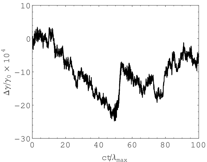
Figure 1: The fractional change in particle energy $\Delta\gamma/\gamma_{0}$ as a function of time for a $\gamma_{0}=10^{6}$ particle injected into an intercloud-like environment ($B_{0}=50\,\mu$G, $v_{A}=35$ km/s) with an Alfvénic turbulent field defined by the parameters $\lambda_{max}=1$ pc, $\lambda_{min}=0.002$ pc, $\Gamma=3/2$, $\xi=2.0$, and $N_{k}=25$.

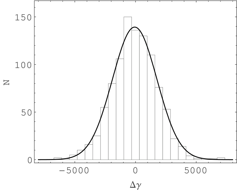
Figure 2: The particle energy distribution for the ensemble of $N_{p}=1,000$ particles at time $t=100\lambda_{max}/c$ in our baseline numerical experiment (Experiment 1). The solid line shows a Gaussian fit to the data.

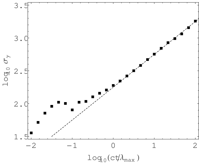
Figure 3: The variance of the particle energy distribution as a function of time for the $N_{p}=1,000$ particles in our baseline numerical experiment (Experiment 1). The dotted line serves as a reference and has a slope of $1/2$, clearly indicating that $\sigma_{\gamma}\propto\sqrt{t}$ for time $t\gtrsim\lambda_{max}/c$.

The spatial diffusion of particles will be different in the parallel and perpendicular directions to the underlying magnetic field $B_{0}\hat{z}$, resulting in different variances in the distributions of particle displacement along and across the underlying field. To illustrate this point, we plot $\sigma_{x}\equiv\sqrt{\langle\Delta x^{2}\rangle}$ and $\sigma_{z}\equiv\sqrt{\langle\Delta z^{2}\rangle}$ as a function of time in Figure 4 for the particles in our baseline experiment. As expected, particles diffuse farther in the direction parallel to the magnetic field, and both output measures become $\propto\sqrt{t}$ at time $t\gtrsim\lambda_{max}/c$.

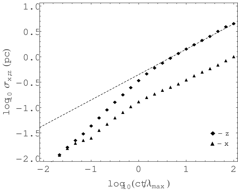
Figure 4: The variance of the particle spatial distributions perpendicular ($x$) and parallel ($z$) to the underlying field $\vec{B}_{0}$ as a function of time for the $N_{p}=1,000$ particles in our baseline numerical experiment (Experiment 1). The dotted line serves as a reference and has a slope of $1/2$, clearly indicating that $\sigma_{x}$ and $\sigma_{z}$ are proportional to $\sqrt{t}$ for time $t\gtrsim\lambda_{max}/c$.

A fundamental issue in this analysis is what value of $N_{k}$ will allow our discrete treatment of the turbulent field to adequately represent the continuous fields found in nature. Toward that end, we repeated our baseline experiment with $N_{k}$ = 250. The difference in output measures were smaller than 10%, indicating that setting $N_{k}=25$ provides good accuracy in our results. We also repeated our baseline experiment with $\lambda_{min}=0.0002$ pc. Again, the difference in output measures were smaller than 10%, indicating that our output measures are not sensitive to the value of $\lambda_{min}$ so long as the particle radius of gyration $R_{g}>\lambda_{min}$ (see also Fatuzzo et al. 2010).

Guided by the results of our baseline analysis, we will perform the remainder of our experiments using $N_{k}=25$ and $\lambda_{min}=0.1R_{g0}$, where

$$R_{g0}={\gamma_{0}m_{p}c^{2}\over eB_{0}}\;,$$ (13)

is the radius of gyration for the injected particles in the absence of turbulence. The governing equations for each particle will be integrated out to a time sufficiently long to ensure that $\sigma_{\gamma}$, $\sigma_{x}$ and $\sigma_{z}$ are proportional to $\sqrt{t}$ by the end of the integration (usually $\Delta t=100\lambda_{max}/c$), and the particles have therefore fully sampled the turbulent nature of the magnetic and electric fields. This scheme is expected to provide accurate results with minimal computing resources.

As a consistency check, we perform a set of experiments (2 – 7) using the same physical conditions corresponding to models W3 and X3 presented in O’Sullivan et al. (2009; see Table 1 and Figures 3 and 4). Specifically, we consider a physical environment defined by the parameters $B_{0}=3\,\mu$G and $v_{A}=0.002$ c, and a turbulent field defined by $\Gamma=5/3$ (Kolmogorov) and $\lambda_{max}=1$ kpc for $\xi=0.2$ (corresponding to model W3 for which $\langle\delta B/B_{0}\rangle^{2}=0.1$) and $\xi=2$ (corresponding to model X3 for which $\langle\delta B/B_{0}\rangle^{2}=1$). We compare our results for the acceleration time $\tau_{acc}$ to those obtained by O’Sullivan et al. (2009) in Figure 5. While there is general agreement between these results, our values of the acceleration times are consistently about a factor of two greater than those to which we are comparing.

As a final consistency check, we compare in Figure 6 the spatial diffusion coefficients $D_{\perp}$ and $D_{||}$ obtained for Exp. 5 – 7 to those obtained by Fatuzzo et al. (2010) under the same physical conditions. We note that the turbulent magnetic field used in our earlier work is of the form given by Equation 1, but with

$$\vec{A}_{n}=A_{n}\left(\cos\alpha_{n}\;\hat{y}^{\prime}\pm i\sin\alpha_{n}\;\hat{z}^{\prime}\right)\;,$$ (14)

where the $y^{\prime}-z^{\prime}$ plane is normal to the $\vec{k}$ direction and $\alpha_{n}$ is picked at random for each $n$ term. As can be seen from Figure 6, there is good agreement between results, indicating that the turbulent magnetic field adopted in this work is equivalent to that used in our earlier work. We note also that the presence of a weak turbulent electric field (i.e., $\delta E<<\delta B$), which was not included in the calculations of Fatuzzo et al. (2010), has a negligible effect on the spatial diffusion of particles.

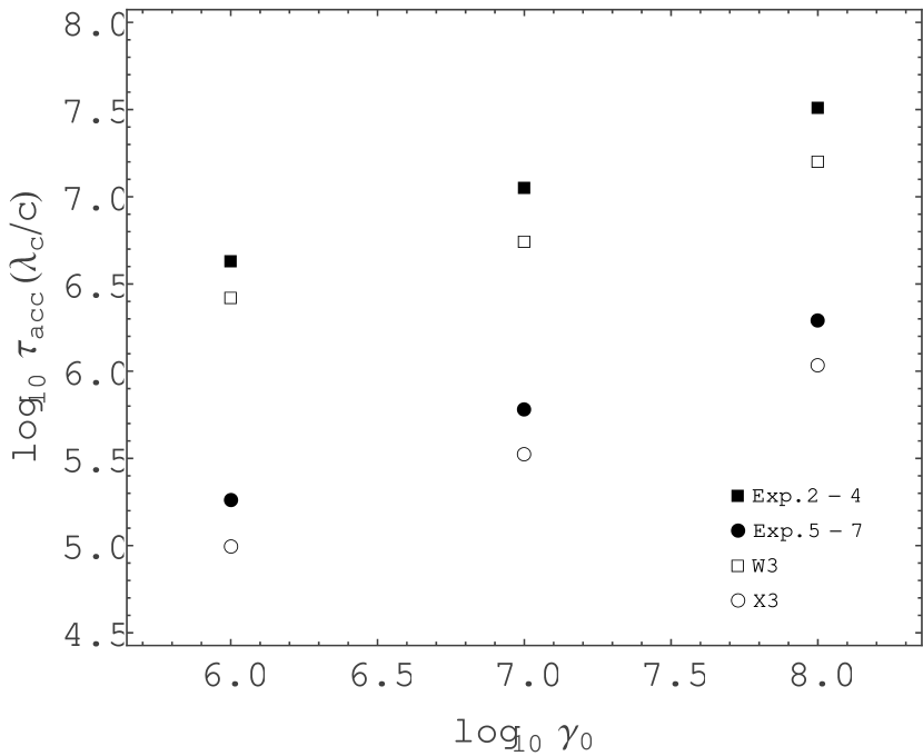
Figure 5: Acceleration time $\tau_{acc}$ as a function of the injected particle Lorentz factor, for both our work and the work of O’Sullivan et al. (2009). Open squares (W3) and circles (X3) denote the results of O’Sullivan et al. (2009). Solid squares and circles denote our results. We note that $\lambda_{c}=0.77\lambda_{max}/(2\pi)$.

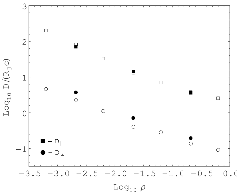
Figure 6: Diffusion coefficients $D_{\perp}$ and $D_{||}$ as a function of rigidity $\rho=2\pi R_{g0}/\lambda_{max}$ for experiments 5 – 7 [solid squares and circles] compared with results obtained by Fatuzzo et al. (2010) for which $\xi=2$ (open squares and circles).

4.2 Survey of Parameter Space

As noted above, the spatial and energy diffusion of particles through turbulent fields is not sensitive to the minimum wavelength so long as the particle’s radius of gyration exceeds $\lambda_{min}$. For a given environment, as defined by $B_{0}$ and $v_{A}$, the diffusion process is thus dependent upon the maximum turbulence wavelength $\lambda_{max}$, the turbulent field strength, as characterized by $\xi$, and the turbulence spectrum, as characterized by the spectral index $\Gamma$.

Quasi-linear theory predicts that the energy diffusion coefficient for relativistic particles scales as

$$D_{\gamma}\approx{v_{A}^{2}\over c^{2}}\,{\delta B^{2}\over B_{0}^{2}}\left({R_{g}\over\lambda_{max}}\right)^{\Gamma-1}{p^{2}c^{2}\over R_{g}c}\,,$$ (15)

where $p$ is the particle momentum (Schlickeiser 1989). For relativistic particles, the energy diffusion coefficient should therefore scale to our model parameters as

$$D_{\gamma}\propto\xi\,\lambda_{max}^{1-\Gamma}\,\gamma_{0}^{\Gamma}\,.$$ (16)

Equation (15) however does not appear to be valid in the strong turbulence limit (O’Sullivan et al. 2009). We therefore investigate how the energy diffusion coefficient depends upon $\lambda_{max}$ and $\xi$ for Kolmogorov ($\Gamma=5/3$) turbulence. Specifically, we perform two sets of experiments designed to explore parameter space around our baseline values. For the first set (Experiments 8 – 10), we vary $\lambda_{max}$ from 0.32 – 10 pc, while in the second set (Experiments 11 – 13) we vary $\xi$ between 0.2 – 6.4.

The energy diffusion coefficients for Experiments 1 and 8 – 10 are presented in Figure 7, with the best line fit to the data indicating that $D_{\gamma}\propto\lambda_{max}^{-0.47}$. This results confirms that quasi-linear theory, which predicts that $D_{\gamma}\propto\lambda_{max}^{-0.67}$ for Kolmogorov turbulence, is not applicable in the strong turbulence ($\xi\gtrsim 1$) limit. The energy diffusion coefficients for Experiments 1 and 8 – 10 are presented in Figure 8, with the best line fit to the data indicating that $D_{\gamma}\propto\xi^{1.2}$ in both the weak and strong turbulence limit.

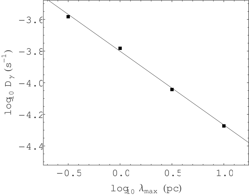
Figure 7: The energy diffusion coefficients $D_{\gamma}$ as a function of maximum turbulence wavelength $\lambda_{max}$ for experiments 1 and 8 – 10. The best line fit to the data has a slope of $-0.47$.

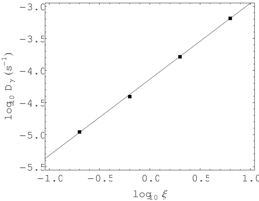
Figure 8: The energy diffusion coefficients $D_{\gamma}$ as a function of $\xi$ for experiments 1 and 11 – 14. The best line fit to the data has a slope of $1.2$.

5 Application to the GC Environment

The stochastic acceleration of protons in a magnetically turbulent environment is essentially a 1-D random walk process that results in a particle energy distribution that broadens in time. Our goal in this section is to calculate the characteristic particle energy for both the inter-cloud medium and the molecular cloud region observed at the GC. As shown in §4, a numerical treatment of particle diffusion requires an integration time-step $\delta t\sim$$0.1\lambda_{min}\sim$$0.01R_{g}$, but a total integration time that is $\Delta t\sim$$100\lambda_{max}$. Numerically integrating the equations of motion for protons that are energized from a thermal state to TeV energies is therefore not computationally feasible given the small radius of gyration of thermal particles.

As such, we determine the characteristic particle energy in each region by comparing the “acceleration time” $\tau_{acc}=\gamma_{0}^{2}/D_{\gamma}$, which characterizes how long it would take a distribution of low-energy particles to attain energies $\sim$$\gamma_{0}m_{p}c^{2}$, with the escape time $\tau_{esc}=R^{2}/D_{||}$, which characterizes how long it would take those particles to diffuse a distance $R$ along the preferential $\hat{z}$ direction, and the proton cooling time $\tau_{pp}$, which characterizes how long a proton can move through a region before losing a significant fraction of its energy to $pp$ scattering with the ambient medium.

To determine how the acceleration and escape times depend on particle energy for the inter-cloud medium ($B_{0}=50\,\mu$G, $v_{A}=35$ km/s, $R=200$ pc), we perform a set of Experiments (14 – 18) using our base-line parameters $\Gamma=5/3$, $\lambda_{max}=1$ pc, and $\xi=2$. We perform two additional experiments (19 & 20) at $\gamma_{0}=10^{5}$ and $\gamma_{0}=10^{6}$ for the same environment, but with $\Gamma=3/2$. We perform a final set of Experiments (21 – 26) to determine how the acceleration and escape times depend on particle energy for the molecular cloud medium ($B_{0}=500\,\mu$G, $v_{A}=11$ km/s, $R=30$ pc).

The energy loss rate of protons with energies needed to produce $\pi^{0}$-decay $\gamma$-rays is dominated by nuclear energy losses due to $pp$ scattering with the ambient medium (Aharonian & Atoyan 1996). As such, the cooling time, $\tau_{pp}$, of the protons depends on the pp-scattering cross-section, $\sigma_{pp}$, and the inelasticity parameter, $\kappa$. Over a broad range of proton energies, neither of these quantities significantly varies so the usual method is to adopt the constant average values $\sigma_{pp}\approx$ 40 mb and $\kappa\approx$ 0.45 (see, e.g., Markoff et al. 1997). That being the case, the proton cooling time becomes independent of proton energy:

$$\tau_{pp}=(n_{H}c\kappa\sigma_{pp})^{-1}\;,$$ (17)

where $n_{H}$ is the number density of ambient protons. The value of $\tau_{pp}$ is therefore $\approx 2\times 10^{14}$ s for the inter-cloud region and $\approx 2\times 10^{11}$ within the molecular cloud region.

Our principal results are presented in Figures 9 and 10. A characteristic particle energy for each region can be estimated by the crossing point where $\tau_{acc}$ becomes greater than either $\tau_{esc}$ or $\tau_{pp}$. Interestingly, this value is $\sim$$3$ Tev for the intercloud region, indicating that the TeV cosmic-rays associated with the HESS observations can thus be produced via stochastic acceleration within the turbulent intercloud environment. This result appears to hold true for both Kolmogorov ($\Gamma=5/3$) and Kraichnan ($\Gamma=3/2$) turbulence, and suggests that energy diffusion in the strong turbulence limit is not sensitive to the turbulence power-spectrum. In contrast, while the acceleration time associated with the molecular clouds are comparable to those in the intercloud medium, the escape time and the proton cooling time are significantly shorter. As such, it is clear from Figure 10 that TeV protons cannot be energized within the molecular cloud environment.

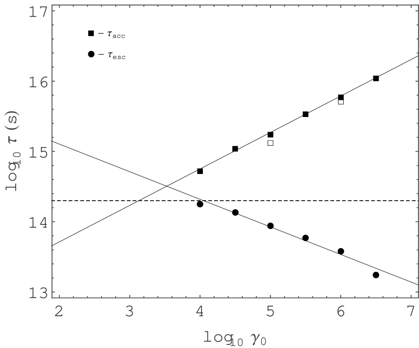
Figure 9: The acceleration time $\tau_{acc}$ and escape time $\tau_{esc}$ for the intercloud environment as a function of injection energy (as characterized by the Lorentz factor $\gamma_{0}$) for experiments 14 – 20 (solid squares and circles) and experiments 19 – 20 (open squares). The solid lines represent the best-line fits to the data from experiments 14 – 20, and the dashed line represents the value of $\tau_{pp}$ in the intercloud region .

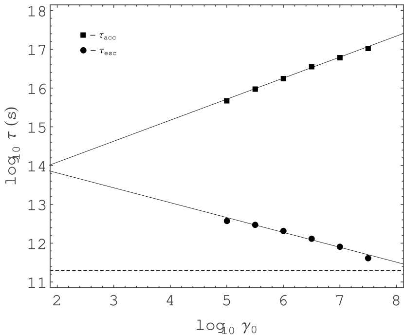
Figure 10: The acceleration time $\tau_{acc}$ and escape time $\tau_{esc}$ for the molecular cloud environment as a function of injection energy (as characterized by the Lorentz factor $\gamma_{0}$) for experiments 21 – 26. The solid lines represent the best-line fits to the data, and the dashed line represents the value of $\tau_{pp}$ in the GC molecular clouds.

6 Conclusion

The purpose of this paper has been to assess the feasibility of stochastic acceleration within the GC region in producing the TeV cosmic-rays revealed by the diffuse HESS emission correlated with the molecular gas distributed along the GC ridge. As shown in previous work, this emission can be produced by cosmic rays with an energy distribution that has a high-energy tail extending out beyond a few TeV. Such a distribution is naturally produced by the stochastic acceleration of particles in a magnetically turbulent environment (which is effectively a 1-D random walk in energy). Thus, the remaining question is whether or not this mechanism is efficient enough to energize protons to the required TeV energies in the highly conductive interstellar medium permeating the galactic center.

To resolve this issue, we performed a series of numerical experiments in order to calculate the spatial and energy diffusion coefficients for protons in both the molecular cloud and the intercloud medium located within the inner several hundred parsecs of the galaxy. We then estimated the characteristic energy of the resulting particle distribution by comparing the acceleration time required for particles to reach a certain energy, the escape time which characterizes how long it takes protons to diffuse out of each region, and the cooling time which characterizes how long a proton can move through a region before losing a significant fraction of its energy to $pp$ scattering with the ambient medium.

Our results indicate that for the physical conditions observed in the intercloud medium, together with reasonable estimates of the turbulent field strength and maximum turbulence wavelength, protons can be accelerated to characteristic energies $\sim$$3$ TeV, indicating that the TeV cosmic-rays observed by HESS can thus be produced via stochastic acceleration within the turbulent intercloud environment. In contrast, while the acceleration time associated with the molecular clouds are comparable to those in the intercloud medium, the escape time and the proton cooling time are significantly shorter. As such, protons cannot be energized to TeV energies within the molecular cloud environment.

These results are very encouraging, not only because the idea of stochastic acceleration in a turbulent magnetic field at the GC appears to be a viable mechanism for producing the cosmic rays observed in that region, but especially because the characteristic energy attained by the relativistic protons matches the observations very well. We note, in this regard, that the physical conditions used in our simulations are unique to the GC. As such, cosmic rays like those observed by HESS are not easily produced by this mechanism anywhere else in the Galaxy.

So the investigation now turns to the very important subsequent question, which we already alluded to in the introduction, viz. can we understand the origin of cosmic rays observed at Earth, at least up to energies $\sim$3–5 TeV, as the result of stochastic acceleration at the GC followed by energy-dependent diffusion and escape across the Milky Way? Simulations designed to address this issue are currently underway, and the results will be reported elsewhere.

Table 1: Summary of Experiments

Exp	$B_{0}$ ($\mu$G)	$v_{A}$ (km/s)	$\Gamma$	$\lambda_{\rm max}$    (pc)	$\xi$	$\gamma_{0}$	$D_{\gamma}$ (s-1)	$D_{\perp}$ (cm2 s-1)	$D_{||}$ (cm2 s-1)
1	50	$35$	$5/3$	1	2	$10^{6}$	$1.6\times 10^{-4}$	$4.9\times 10^{26}$	$9.8\times 10^{27}$
2	3	$600$	$5/3$	$10^{3}$	0.2	$10^{8}$	$2.4\times 10^{-2}$	$1.4\times 10^{29}$	$2.6\times 10^{32}$
3	3	$600$	$5/3$	$10^{3}$	0.2	$10^{7}$	$6.8\times 10^{-4}$	$9.4\times 10^{28}$	$1.2\times 10^{32}$
4	3	$600$	$5/3$	$10^{3}$	0.2	$10^{6}$	$1.8\times 10^{-5}$	$7.0\times 10^{28}$	$6.6\times 10^{31}$
5	3	$600$	$5/3$	$10^{3}$	2	$10^{8}$	$3.9\times 10^{-1}$	$6.2\times 10^{29}$	$1.2\times 10^{31}$
6	3	$600$	$5/3$	$10^{3}$	2	$10^{7}$	$1.3\times 10^{-2}$	$2.3\times 10^{29}$	$4.6\times 10^{30}$
7	3	$600$	$5/3$	$10^{3}$	2	$10^{6}$	$4.2\times 10^{-4}$	$1.2\times 10^{29}$	$2.3\times 10^{30}$
8	50	$35$	$5/3$	0.32	2	$10^{6}$	$2.6\times 10^{-4}$	$2.6\times 10^{26}$	$6.7\times 10^{27}$
9	50	$35$	$5/3$	3.2	2	$10^{6}$	$9.2\times 10^{-5}$	$9.3\times 10^{26}$	$1.8\times 10^{28}$
10	50	$35$	$5/3$	10	2	$10^{6}$	$5.4\times 10^{-5}$	$1.7\times 10^{27}$	$4.2\times 10^{28}$
11	50	$35$	$5/3$	1	0.2	$10^{6}$	$1.1\times 10^{-5}$	$1.4\times 10^{26}$	$2.1\times 10^{29}$
12	50	$35$	$5/3$	1	0.64	$10^{6}$	$4.0\times 10^{-5}$	$2.9\times 10^{26}$	$4.6\times 10^{28}$
13	50	$35$	$5/3$	1	6.4	$10^{6}$	$6.6\times 10^{-4}$	$6.9\times 10^{26}$	$2.6\times 10^{27}$
14	50	$35$	$5/3$	1	2	$3.2\times 10^{6}$	$8.7\times 10^{-4}$	$8.4\times 10^{26}$	$2.1\times 10^{28}$
15	50	$35$	$5/3$	1	2	$3.2\times 10^{5}$	$2.9\times 10^{-5}$	$2.9\times 10^{26}$	$6.3\times 10^{27}$
16	50	$35$	$5/3$	1	2	$10^{5}$	$5.6\times 10^{-6}$	$2.0\times 10^{26}$	$4.3\times 10^{27}$
17	50	$35$	$5/3$	1	2	$3.2\times 10^{4}$	$1.0\times 10^{-6}$	$1.3\times 10^{26}$	$2.8\times 10^{27}$
18	50	$35$	$5/3$	1	2	$10^{4}$	$1.9\times 10^{-7}$	$9.6\times 10^{25}$	$2.1\times 10^{27}$
19	50	$35$	$3/2$	1	2	$10^{6}$	$1.9\times 10^{-4}$	$3.9\times 10^{26}$	$9.6\times 10^{27}$
20	50	$35$	$3/2$	1	2	$10^{5}$	$7.5\times 10^{-6}$	$1.3\times 10^{26}$	$2.3\times 10^{27}$
21	500	$11$	$5/3$	1	2	$3.2\times 10^{7}$	$9.1\times 10^{-3}$	$8.6\times 10^{26}$	$2.0\times 10^{28}$
22	500	$11$	$5/3$	1	2	$10^{7}$	$1.6\times 10^{-3}$	$4.5\times 10^{26}$	$1.0\times 10^{28}$
23	500	$11$	$5/3$	1	2	$3.2\times 10^{6}$	$2.7\times 10^{-4}$	$2.8\times 10^{26}$	$6.3\times 10^{27}$
24	500	$11$	$5/3$	1	2	$10^{6}$	$5.5\times 10^{-5}$	$2.0\times 10^{26}$	$4.0\times 10^{27}$
25	500	$11$	$5/3$	1	2	$3.2\times 10^{5}$	$1.0\times 10^{-5}$	$1.4\times 10^{26}$	$2.8\times 10^{27}$
26	500	$11$	$5/3$	1	2	$10^{5}$	$2.1\times 10^{-6}$	$1.1\times 10^{26}$	$2.2\times 10^{27}$

References

- aharonian (96) Aharonian, F. A., & Atoyan, A. M. 1996, A&A, 309, 917
- aha (06) Aharonian, F. et al. 2006, Nature, 439, 695
- Aronmax (1975) Arons, J., & Max, C. E. 1975, ApJ, 196, L77
- bal (07) Ballantyne, D., Melia, F., & Liu, S. 2007, ApJ Letters, 657, L13
- casetal (02) Casse, F., Lemoine, M., & Pelletier, G. 2002, PhRvD, 65, 023002
- croc (05) Crocker, R., Fatuzzo, M., Jokipii, R., Melia, F., and Volkas, R. 2005, ApJ, 622, 892
- croc (10) Crocker, R. M., Jones, D. I., Melia, F., Ott, J., and Protheroe, R. J. 2010, Nature, 463, 65
- Crutcher (1998) Crutcher, R. M. 1998, in Interstellar Turbulence, eds. J. Franco and J. Carraminana (Cambridge: Cambridge Univ. Press), pp. 213
- Crutcher (1999) Crutcher, R. M. 1999, ApJ, 520, 706
- Fatuzzo & Adams (1993) Fatuzzo, M., & Adams, F. C. 1993, ApJ, 412, 146
- fat (10) Fatuzzo, M., Melia, F., Todd, E., and Adams, F. C. 2010, ApJ, 725, 515
- fat (11) Fatuzzo, M., and Melia, F. 2011, MNRAS Letters, 410, L23
- gammie (1996) Gammie, C. F., & Ostriker, E. C. 1996, ApJ, 466, 814
- giajok (94) Giacalone, J. & Jokipii, J. R. 1994, ApJL, 430, L137
- gust (04) Güsten, R., and Philipp, S. 2004, arXiv:astro-ph/0402019
- hun (97) Hunter, S. D., et al. 1997, ApJ, 481, 205
- larosa (05) LaRosa, T. N. et al. 2005, ApJ Letters, 626, L23
- larson (1985) Larson, R. B. 1981, MNRAS, 194, 809
- (19) McKee, C. F., & Zweibel, E. G. 1995, ApJ, 440, 686
- Mouschovias (1995) Mouschovias, T. Ch., & Psaltis, D. 1995, ApJ, 444, L105
- mor (89) Morris, M., and Yusef-Zadeh, F. 1989, ApJ, 343, 703
- mor (07) Morris, M. 2007, arXiv:astro-ph/0701050
- (23) Myers, P. C., & Gammie, C. F. 1999, ApJ, 522, 141
- Myers & Goodman (1988) Myers, P. C., & Goodman, A. A. 1988, ApJ, 326, L27
- (25) Myers, P. C., & Ladd, E. F., & Fuller, G. A. 1991, ApJ, 372, 95
- osuetal (09) O’Sullivan, S., Reville, B., & Taylor, A. M. 2009, MNRAS, 400, 248
- rock (04) Rockefeller, G., Fryer, C. L., Melia, F., and Warren, M. S., 2004, ApJ, 604, 662
- schlick (89) Schlickeiser, R., 1989, ApJ, 336, 243
- tsu (99) Tsuboi, M., Toshihiro, H., and Ukita, N. 1999, ApJ Supplements, 120, 1
- walm (86) Walmsley, C. et al. 1986, A&A, 155, 129
- wom (08) Wommer, E., Melia, F., and Fatuzzo, M. 2008, MNRAS, 387, 987
- yus (87) Yusef-Zadeh, F., and Morris, M. 1987, AJ, 94, 1178