A report on the nonlinear squeezed states and their non-classical properties of a generalized isotonic oscillator

Abstract

We construct nonlinear squeezed states of a generalized isotonic oscillator potential. We demonstrate the non-existence of dual counterpart of nonlinear squeezed states in this system. We investigate statistical properties exhibited by the squeezed states, in particular Mandel’s parameter, second-order correlation function, photon number distributions and parameter $A_{3}$ in detail. We also examine the quadrature and amplitude-squared squeezing effects. Finally, we derive expression for the $s$-parameterized quasi-probability distribution function of these states. All these information about the system are new to the literature.

1 Introduction

Very recently studies have been made to analyze the generalized isotonic oscillator potential, $V(y)=\left(\frac{m_{0}\omega^{2}}{2}y^{2}+\frac{g_{a}(y^{2}-a^{2})}{(y^{2}+a^{2})^{2}}\right)$, in different perspectives [1, 2, 3, 4, 5, 6, 7, 8, 9, 10, 11]. The associated Schrödinger equation can be written as (after suitable rescaling)

$$-\frac{1}{2}\frac{d^{2}\psi_{n}(x)}{dx^{2}}+\frac{1}{2}\left(x^{2}+\frac{8(2x^{2}-1)}{(2x^{2}+1)^{2}}\right)\psi_{n}(x)=E_{n}\psi_{n}(x).$$ (1)

Equation (1) admits eigenfunctions and energy eigenvalues as [1]

$$\psi_{n}(x) = {\cal N}_{n}\displaystyle{\frac{{\cal P}_{n}(x)}{(1+2x^{2})}}e^{\displaystyle-{x^{2}}/2},$$ (2)

$$E_{n} = -\frac{3}{2}+n,\quad\qquad\qquad n=0,3,4,5,...,$$ (3)

where the polynomial factors ${\cal P}_{n}(x)$ are given by

$$\qquad\qquad{\cal P}_{n}(x)=\left\{\begin{array}[]{c}1,\quad\qquad\qquad\qquad\qquad\qquad\qquad\qquad\quad\mbox{if}\;\;n=0\\ H_{n}(x)+4nH_{n-2}(x)+4n(n-3)H_{n-4}(x),\;\mbox{if}\;\;n=3,4,5,...\\ \end{array}\right.$$ (6)

and the normalization constant

$${\cal N}_{n}=\left[\displaystyle{\frac{(n-1)(n-2)}{2^{n}n!\sqrt{\pi}}}\right]^{1/2},\quad n=0,3,4,5,....$$ (7)

We consider (1) as the number operator equation after subtracting the ground state energy ${\displaystyle E_{0}=-\frac{3}{2}}$ from it, that is

$$\hat{N}_{0}|n\rangle=n|n\rangle.$$ (8)

In a very recent paper [9], we have addressed the method of finding the deformed ladder operators $\hat{N}_{-}$ and $\hat{N}_{+}$ from the solution (2). The deformed ladder operators $\hat{N}_{-}$ and $\hat{N}_{+}$ satisfy the relations [9]

$$\hat{N}_{-}|n\rangle = \sqrt{n}\;f(n)\;|n-1\rangle,$$ (9)

$$\hat{N}_{+}|n\rangle = \sqrt{n+1}\;f(n+1)\;|n+1\rangle,$$ (10)

with $f(n)=\sqrt{(n-1)(n-3)}$. Since $f(n)$ has zeros at $n=1$ and $3$, we relate the annihilation ($\hat{a}$) and creation operators ($\hat{a}^{\dagger}$) to the deformed ladder operators $\hat{N}_{-}$ and $\hat{N}_{+}$ through the relations,

$$\hat{a}=\frac{1}{f(\hat{N}_{0}+1)}\hat{N}_{-},\qquad\hat{a}^{\dagger}=\frac{1}{f(\hat{N}_{0})}\hat{N}_{+},\quad n=0,3,4,5,...$$ (11)

in which we preserve the ordering of operators $f(\hat{N}_{0}),\;\hat{N}_{-}$ and $\hat{N}_{+}$. Specifically the operators $\hat{a}$ and $\hat{a}^{\dagger}$ act on the states $|0\rangle$ and $|3\rangle$ yield

$$\hat{a}|0\rangle = \frac{1}{f(\hat{N}_{0}+1)}\hat{N}_{-}|0\rangle=0,\qquad\hat{a}^{\dagger}|0\rangle=\frac{1}{f(\hat{N}_{0})}\hat{N}_{+}|0\rangle=0,$$ (12)

$$\hat{a}|3\rangle = \frac{1}{f(\hat{N}_{0}+1)}\hat{N}_{-}|3\rangle=0,\qquad\hat{a}^{\dagger}|3\rangle=\frac{1}{f(\hat{N}_{0})}\hat{N}_{+}|3\rangle=\sqrt{4}\;|4\rangle.$$ (13)

For the remaining states, the operators produce

$$\hat{a}|n\rangle = \sqrt{n}\;|n-1\rangle,$$ (14)

$$\hat{a}^{\dagger}|n\rangle = \sqrt{n+1}\;|n+1\rangle,\quad n=4,5,6,7,...$$ (15)

and $\hat{N}_{0}=\hat{a}^{\dagger}\hat{a}$.

Since $\hat{N}_{-}|0\rangle=0$ and $\hat{N}_{+}|0\rangle=0$, the ground state can be considered as an isolated one. Further, the expression $\hat{N}_{-}|3\rangle=0$ implies that the first excited state $|3\rangle$ acts as a ground state. This is due to the reason that $f(n)$ has zeros at $n=1$ and $3$. Because of this fact, the Hilbert space ${\cal H}$ consists of states $|0\rangle,|3\rangle,|4\rangle,...$ splits up into two invariant sub-spaces, namely (i) $|\Psi\rangle=|0\rangle$ and (ii) $|\Psi^{{}^{\prime}}\rangle=\sum^{\infty}_{n=3}c_{n}|n\rangle$ for the operators $\hat{N}_{-}$ and $\hat{N}_{+}$ [12]. We consider the sub-Hilbert space, ${\cal H^{\prime}}$, spanned by the eigenstates, $|3\rangle,|4\rangle,|5\rangle,...$ and exclude the ground state $|0\rangle$ for further discussion.

The operators $\{\hat{N}_{-},\hat{N}_{+},\hat{N}_{0}\}$ satisfy the following deformed $su(1,1)$ algebra [10, 13, 14]

$$[\hat{N}_{+},\hat{N}_{-}]|n\rangle=[5\hat{N}_{0}-3\hat{N}^{2}_{0}]|n\rangle,\qquad\;[\hat{N}_{0},\hat{N}_{\pm}]|n\rangle=\pm\hat{N}_{\pm}|n\rangle$$ (16)

with Casimir operator of the type [15]

$$\hat{C}=\hat{N}_{-}\hat{N}_{+}+h(\hat{N}_{0})=\hat{N}_{+}\hat{N}_{-}+h(\hat{N}_{0}-1),$$ (17)

where $h(\hat{N}_{0})$ is a real function which is of the form [15]

$$h(\hat{N}_{0})=\frac{5}{2}\hat{N}_{0}(\hat{N}_{0}+1)-\hat{N}_{0}(\hat{N}_{0}+1)(\hat{N}_{0}+\frac{1}{2}).$$ (18)

We note here that a physical interpretation for the deformed operators was already given in Refs. [12, 16]. In the present case also, we observe that the frequency of vibrations of the nonlinear oscillator depends on the energy of vibrations. To demonstrate this let us consider the Hamiltonian $\tilde{H}=\frac{1}{2}\left(\hat{N}_{+}\hat{N}_{-}+\hat{N}_{-}\hat{N}_{+}\right)$ associated with the quantum $f$-deformed nonlinear oscillator. The energy eigenvalues in the Fock space is then given by $\tilde{E}_{n}=\frac{1}{2}[n(1-5n+2n^{2})]$ [12, 16]. The Heisenberg equation of motion for $\hat{N}_{-}$ (or $\hat{N_{+}}$) now reads

$$\dot{\hat{N}}_{-}+i[\hat{N}_{-},\tilde{H}(\hat{N}_{0})]=0\;\Rightarrow\;\dot{\hat{N}}_{-}+i\omega_{\pm}(\hat{N}_{0})\hat{N}_{-}=0,$$ (19)

where $\omega_{+}(\hat{N}_{0})=\tilde{H}(\hat{N}_{0}+1)-\tilde{H}(\hat{N}_{0})=3\hat{N}^{2}_{0}-2\hat{N}_{0}-1$, $\omega_{-}(\hat{N}_{0})=\tilde{H}(\hat{N}_{0})-\tilde{H}(\hat{N}_{0}-1)=3\hat{N}^{2}_{0}-4\hat{N}_{0}+2$ and the square bracket denotes the usual commutator. In terms of the evolution operator, $U(t)=e^{i\tilde{H}(\hat{N}_{0})(t-t_{0})}$, the solution to (19) can be written as

$$\hat{N}_{-}(t)=e^{-i\omega_{+}(\hat{N}_{0})(t-t_{0})}\hat{N}_{-}(t_{0}).$$ (20)

Expression (20) shows that the quantum $f$-oscillator vibrates with a frequency depends on the energy $\tilde{E}_{n}$.

The aim of this paper is to construct the nonlinear squeezed states of the system (1). A squeezed state is one of the minimum uncertainty states in which the fluctuation of one photon-quadrature component is less than the quantum limit [17]. This can be achieved by increasing or decreasing one of the photon-quadrature dispersions in such a way that the Heisenberg uncertainty relation is not violated [18, 19, 20, 21]. Squeezed states can be produced by acting with the squeezing operator $S(\xi)=\exp{\left(\frac{\xi}{2}\hat{a}^{\dagger^{2}}-\frac{\xi^{*}}{2}\hat{a}^{2}\right)}$ on the coherent state or ground state or first order excited state of a quantum system, where $\hat{a}$ and $\hat{a}^{\dagger}$ are annihilation and creation operators respectively and $\xi$ is a complex parameter. The method of constructing nonlinear squeezed states in the $su(1,1)$ algebra was discussed in Ref. [22]. The nonlinear squeezed states [23] have applications in quantum cryptography [24], quantum teleportation [25] and moreover they have also been proposed for high precision measurements such as improving the sensitivity of Ramsey fringe interferometry [26] . During the past three decades considerable efforts have been made towards the methods of generating squeezed states in particular optical four-wave mixing and optical fibers, parametric amplifiers, non-degenerate parametric oscillators and so on [19, 27, 28, 29, 30].

Motivated by these recent developments we intend to construct nonlinear squeezed states for the generalized isotonic oscillator potential. By transforming the deformed ladder operators suitably we identify the Heisenberg algebra and the squeezing operators. While one of the operators produces nonlinear squeezed states the other one fails to produce another set of nonlinear squeezed states (dual pair) [31]. Besides constructing nonlinear squeezed states we also investigate the non-classical properties exhibited by the nonlinear squeezed states, by investigating Mandel’s parameter, second-order correlation function and parameter $A_{3}$. We examine non-classical nature of the states by evaluating quadrature squeezing and amplitude-squared squeezing. Further, we derive analytical expressions for the $s$-parameterized function for the non-classical states. The partial negativity of the $s$-parameterized function confirm the non-classical properties of the nonlinear squeezed states. All these informations about the system (1) are new to the literature.

We organize our presentation as follows. In the following section, we discuss the method of obtaining Heisenberg algebra from the deformed annihilation and creation operators. In section 3, we construct nonlinear squeezed states from the Heisenberg algebra for this nonlinear oscillator. Consequently, we analyze certain photon statistical properties, normal quadrature squeezing and amplitude-squared squeezing properties exhibited by the nonlinear squeezed states and the harmonic oscillator squeezed states in section 4. Followed by this, in section 5, we study quadrature distribution and quasi-probability distribution function for the dual pairs of nonlinear squeezed states. Finally, we present our conclusions in section 6.

2 Deformed oscillator algebra and transformations [32]

To construct nonlinear squeezed states [23, 33] of (1), we transform $\hat{N}_{-}$ or/and $\hat{N}_{+}$ suitably, such a way that the newly transformed operators satisfy the Heisenberg algebra. We consider all three possibilities in the following.

First let us rescale $\hat{N}_{+}$ as [13]

$$\hat{{\cal N}}_{+}=\hat{N}_{+}F(\hat{C},\hat{N}_{0}),$$ (21)

where $\hat{{\cal N}}_{+}$ is the new deformed ladder operator and $\displaystyle{F(\hat{C},\hat{N}_{0})=\frac{\hat{N}_{0}+\delta}{\hat{C}-h(\hat{N}_{0})}=\frac{\hat{N}_{0}+\delta}{\hat{N}_{-}\hat{N}_{+}}}$, with $\delta$ is a parameter.

We can generate Heisenberg algebra, for the system (1), through the newly deformed ladder operator (21) in the form [32]

$$\mbox{Case: (i)}\;\;[\hat{N}_{-},\hat{{\cal N}}_{+}]|n\rangle=|n\rangle,\;\;[\hat{\cal N}_{+}\hat{N}_{-},\hat{N}_{-}]|n\rangle=-\hat{N}_{-}|n\rangle,\;\;[\hat{\cal N}_{+}\hat{N}_{-},\hat{\cal N}_{+}]|n\rangle=\hat{\cal N}_{+}|n\rangle.$$ (22)

Similarly by rescaling the ladder operator $\hat{N}_{-}$ such a way that

$$\hat{\cal N}_{-}=F(\hat{C},\hat{N}_{0})\hat{N}_{-},$$ (23)

where $\displaystyle{F(\hat{C},\hat{N}_{0})=\frac{\hat{N}_{0}+\delta}{\hat{C}-h(\hat{N}_{0})}=\frac{\hat{N}_{0}+\delta}{\hat{N}_{-}\hat{N}_{+}}}$, we can generate the second set of Heisenberg algebra in the form

$$\mbox{Case: (ii)}\;\;[\hat{\cal N}_{-},\hat{N}_{+}]|n\rangle=|n\rangle,\;\;[\hat{N}_{+}\hat{\cal N}_{-},\hat{\cal N}_{-}]|n\rangle=-\hat{\cal N}_{-}|n\rangle,\;\;[\hat{N}_{+}\hat{\cal N}_{-},\hat{N}_{+}]|n\rangle=\hat{N}_{+}|n\rangle.$$ (24)

The constant $\delta$ in $F(\hat{C},\hat{N}_{0})$ can be fixed by utilizing the commutation relations, $[\hat{N}_{-},\hat{\cal N}_{+}]|3\rangle=|3\rangle$ and $[\hat{\cal N}_{-},\hat{N}_{+}]|3\rangle=|3\rangle$. From these two relations, we find $\delta=-2$ and fix ${\displaystyle F(\hat{C},\hat{N}_{0})=\frac{\hat{N}_{0}-2}{\hat{N}_{-}\hat{N}_{+}}}$.

Finally, one can rescale both the operators $\hat{N}_{+}$ and $\hat{N}_{-}$ simultaneously and evaluate the commutation relations. For example, let us rescale $\hat{N}_{+}$ and $\hat{N}_{-}$ respectively as $\hat{K}_{+}=\hat{N}_{+}G(\hat{C},\hat{N}_{0})$ and $\hat{K}_{-}=G(\hat{C},\hat{N}_{0})\hat{N}_{-}$. The explicit form of $G(\hat{C},\hat{N}_{0})$ can then be found by using the commutation relation $[\hat{K}_{-},\hat{K}_{+}]=\hat{I}$, that is

$$G(\hat{C},\hat{N}_{0})\hat{N}_{-}\hat{N}_{+}G(\hat{C},\hat{N}_{0})-\hat{N}_{+}G^{2}(\hat{C},\hat{N}_{0})\hat{N}_{-}=\hat{I}.$$ (25)

Solving (25) we find $G(\hat{C},\hat{N}_{0})=\sqrt{F(\hat{C},\hat{N}_{0})}$.

With this choice of $G(\hat{C},\hat{N}_{0})$ we can establish

$$\mbox{Case: (iii)}\;[\hat{K}_{-},\hat{K}_{+}]|n\rangle=|n\rangle,\;\;[\hat{K}_{0},\hat{K}_{-}]|n\rangle=-\hat{K}_{-}|n\rangle,\;\;\;[\hat{K}_{0},\hat{K}_{+}]|n\rangle=\hat{K}_{+}|n\rangle,$$ (26)

where $\hat{K}_{0}=\hat{K}_{+}\hat{K}_{-}$. Here $\hat{K}_{0}$ serves as a number operator.

We construct squeezed and nonlinear squeezed states using these three sets of new deformed ladder operators.

3 Nonlinear squeezed states

3.1 Non-unitary squeezing operators and nonlinear squeezed states

The transformed operators $\hat{\cal N}_{+}$ and $\hat{\cal N}_{-}$ which satisfy the commutation relations (22) and (24) help us to define two non-unitary squeezing operators, namely

$$\mbox{Case: (i)}\;\;\;\;S(\beta) = e^{\frac{\beta}{2}\hat{\cal N}^{2}_{+}-\frac{\beta^{*}}{2}\hat{N}^{2}_{-}},$$ (27)

$$\mbox{Case: (ii)}\;\;\;\tilde{S}(\beta) = e^{\frac{\beta}{2}\hat{N}^{2}_{+}-\frac{\beta^{*}}{2}\hat{\cal N}^{2}_{-}}.$$ (28)

By applying these operators on the lowest energy state $|3\rangle$ given in (2), we obtain the nonlinear squeezed states as

$$\;\mbox{Case: (i)}\;\;\;\;\;|\beta,\tilde{f}\rangle = N_{\beta}\sum^{\infty}_{n=0}\frac{\beta^{n}}{2^{n}\;n!}\sqrt{\frac{(2n)!}{(2n+2)!\;(2n+3)!}}\;|2n+3\rangle,$$ (29)

$$\;\mbox{Case: (ii)}\;\;\;\;\widetilde{|\beta,\tilde{f}\rangle} = {\tilde{N}_{\beta}}\sum^{\infty}_{n=0}\frac{\beta^{n}}{2^{n}\;n!}\sqrt{(2n)!(2n+2)!(2n+3)!}\;|2n+3\rangle,$$ (30)

where the normalization constant $N_{\beta}$ and $\tilde{N}_{\beta}$ are given by

$$\;\;\;\;\mbox{Case: (i)}\;\;\;\;N_{\beta}=\left(\sum^{\infty}_{n=0}\frac{|\beta|^{2n}(2n)!}{4^{n}(n!)^{2}(2n+2)!(2n+3)!}\right)^{-1/2},$$ (31)

$$\;\;\;\;\mbox{Case: (ii)}\;\;\;\tilde{N}_{\beta}=\left(\sum^{\infty}_{n=0}{\frac{|\beta|^{2n}\;(2n)!\;(2n+2)!\;(2n+3)!}{4^{n}(n!)^{2}}}\right)^{-1/2}.$$ (32)

The series given in (32) is of the form ${\displaystyle\sum^{\infty}_{n=0}\frac{12|\beta|^{2n}}{[x_{n}]!}}$, with ${\displaystyle x_{n}=\frac{2n}{(2n-1)(2n+1)(2n+2)^{2}(2n+3)}}$ and $[x_{n}]!=x_{n}.x_{n-1}...x_{1}$. One can unambiguously prove that the series given in (32) is a divergent one since for non-zero values of $|\beta|$, the limit yields ${\displaystyle L^{2}=\lim_{n\to\infty}x_{n}=0}$ and consequently it does not meet the necessary condition, $|\beta|<L$ with $L^{2}\neq 0$. Since $\tilde{N}_{\beta}=0$, the dual states (30) do not exist. Hence, we conclude that for the generalized isotonic oscillator one can construct only nonlinear squeezed states and not their dual counterpart.

3.2 Unitary squeezing operator and squeezed states

In the Case (iii) the squeezing operator

$$S(\xi)=e^{\frac{\xi}{2}\hat{K}^{2}_{+}-\frac{\xi^{*}}{2}\hat{K}^{2}_{-}}$$ (33)

is an unitary one. By applying this operator on the lowest energy state $|3\rangle$ given in (2), we get the normalized form of squeezed states as

$$\;\mbox{Case: (iii)}\;\;\;\;|\xi\rangle=S(\xi)|3\rangle=N_{\xi}\sum^{\infty}_{n=0}\frac{\xi^{n}}{2^{n}n!}\sqrt{(2n)!}|2n+3\rangle,$$ (34)

where $N_{\xi}$ can be obtained from the normalization condition $\langle\xi|\xi\rangle=1$. Doing so we find the normalization constant

$$\quad\qquad\qquad\qquad\quad N_{\xi}=\left(\sum^{\infty}_{n=0}\frac{|\xi|^{2n}\;(2n)!}{4^{n}(n!)^{2}}\right)^{-1/2}.$$ (35)

These squeezed states $|\xi\rangle$ are in the same form as that of harmonic oscillator [17]. We will discuss the properties of these states separately hereafter.

4 Non-classical properties

In this section we study certain photon statistical properties, namely (i) the photon number distribution $(P(n))$, (ii) Mandel’s parameter $(Q)$ and (iii) the second-order correlation function $(g^{2}(0))$ associated with the nonlinear squeezed states given in (29) and squeezed states given in (34). In addition to these, we also analyze quadrature and amplitude-squared squeezing for the non-classical states.

4.1 Photon statistical properties

To start with, we calculate the probability of finding $n$ photons in the nonlinear squeezed states (29) which in turn gives

$$\;\;\;\;\mbox{Case: (i)}\;\;\;P(2n)=|\langle 2n+3|\beta,\tilde{f}\rangle|^{2}=\frac{N^{2}_{\beta}|\beta|^{2n}(2n)!}{4^{n}(n!)^{2}\;(2n+2)!\;(2n+3)}.$$ (36)

The photon number distribution for the nonlinear squeezed states $|\beta,\tilde{f}\rangle$ is calculated ($r=|\beta|=20$ with $n_{max}=70$) and plotted in figure 1(a). The result confirms that the distribution is not a Poissonian one.

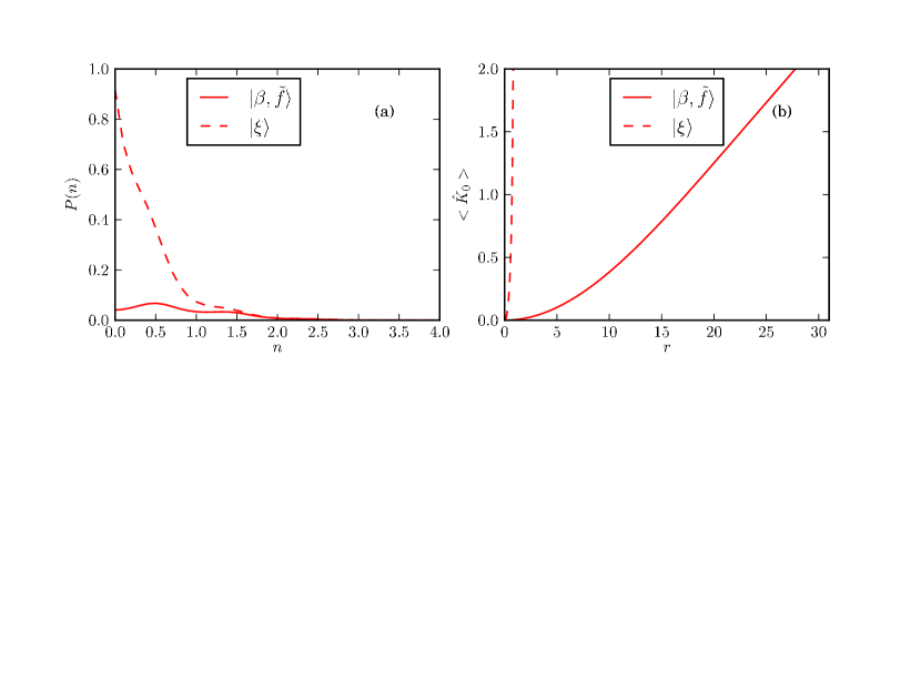
Figure 1: The plots of (a) photon number distribution $P(n)$ and (b) average number of photons $\langle\hat{K}_{0}\rangle$ in nonlinear squeezed states (29) and squeezed states (34)

.

Since $\hat{K}_{+},\hat{K}_{-}$ and $\hat{K}_{0}$ act on the states $|3\rangle,|4\rangle,|5\rangle,...$ in the same way as creation $(\hat{a}^{\dagger})$, annihilation $(\hat{a})$ and number $(\hat{n})$ operators act on the states $|0\rangle,|1\rangle,|2\rangle,...$ of harmonic oscillator potential, we consider $\hat{K}_{0}$ as number operator for the system (1) in the sub-Hilbert space spanned by the eigenstates $|3\rangle,|4\rangle,|5\rangle,...$. So, we examine Mandel’s parameter $Q$ and second-order correlation function $g^{2}(0)$ in terms of $\hat{K}_{0}$ only [34, 35, 36, 37], that is

$$Q=\frac{\langle\hat{K}^{2}_{0}\rangle}{\langle\hat{K}_{0}\rangle}-\langle\hat{K}_{0}\rangle-1,\qquad\;\;\;g^{(2)}(0)=\frac{\langle\hat{K}^{2}_{0}\rangle-\langle\hat{K_{0}}\rangle}{\langle\hat{K}_{0}\rangle^{2}}.$$ (37)

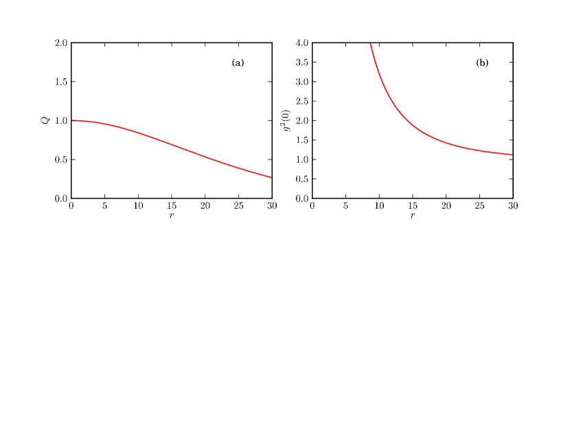
Figure 2: The plots of (a) Mandel’s parameter $Q$ and (b) the second-order correlation function $g^{2}(0)$ of the nonlinear squeezed states (29).

To calculate Mandel’s parameter, we first obtain expressions for $\langle\hat{K}_{0}\rangle$ and $\langle\hat{K}^{2}_{0}\rangle$ corresponding to the nonlinear squeezed states given in (29), which are of the form

$$\mbox{Case: (i)}\;\;\;\langle\hat{K}_{0}\rangle = N^{2}_{\beta}\sum^{\infty}_{n=1}{\frac{|\beta|^{2n}\;(2n-1)!}{4^{n-1}\;((n-1)!)^{2}\;(2n+2)!\;(2n+3)!}},$$ (38)

$$\qquad\qquad\;\langle\hat{K}^{2}_{0}\rangle = N^{2}_{\beta}\sum^{\infty}_{n=1}{\frac{|\beta|^{2n}\;(2n)!}{4^{n-1}\;((n-1)!)^{2}\;(2n+2)!\;(2n+3)!}},$$ (39)

where $\langle\hat{K}_{0}\rangle$ gives the average number of photons in the nonlinear squeezed states $|\beta,\tilde{f}\rangle$ for different values of $r$. The results are plotted in figure 1(b) which demonstrates the nonlinear dependency between $\langle\hat{K}_{0}\rangle$ and $r$.

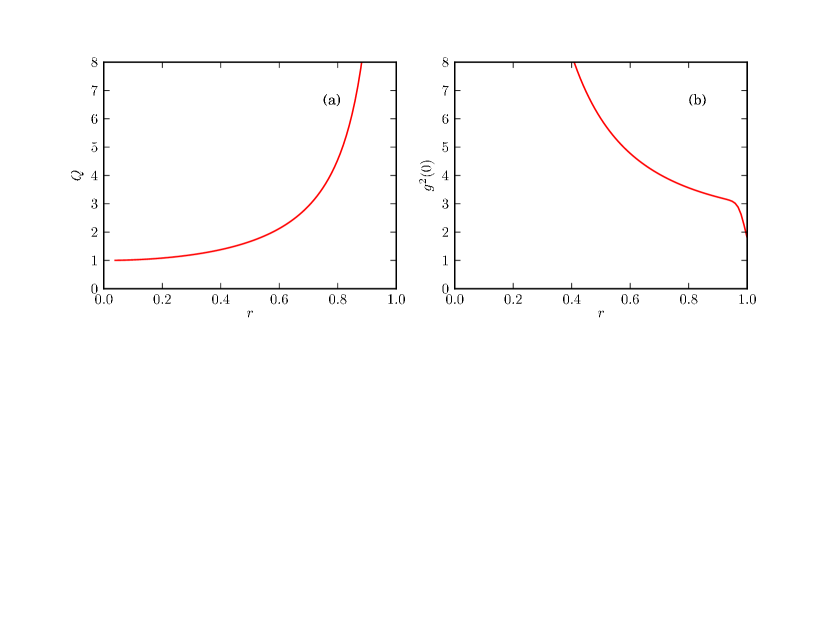
Figure 3: The plots of (a) Mandel’s parameter $Q$ and (b) the second-order correlation function $g^{2}(0)$ of the squeezed states (34).

Substituting the expressions (38)-(39) in (37) and evaluating the resultant expressions we can obtain the Mandel’s parameter and second-order correlation function for the states $|\beta,\tilde{f}\rangle$. Here we investigate the variations of $Q$ and $g^{2}(0)$ against $r(<31)$ and summarize the results in figures 2(a) and 2(b). From the figures we observe that for the values of $r(<31)$ with $n_{max}=70$, $Q>0$ and $g^{2}(0)>1$. The positive values of $g^{2}(0)$ indicate the super-Poissonian nature of the nonlinear squeezed states $|\beta,\tilde{f}\rangle$.

The photon number distribution for the states (34) corresponding to the Case (iii) are found to be

$$\qquad\quad\mbox{Case:\;(iii)}\;\;\;P(2n)=|\langle 2n+3{|\xi,\tilde{f}\rangle}|^{2}=N^{2}_{\xi}\frac{|\xi|^{2n}(2n)!}{4^{n}\;(n!)^{2}},$$ (40)

which is calculated and plotted in figure 1(a) with $r=0.4$ and $n_{max}=70$. As shown in the figure, the photon number distribution for the states $|\xi\rangle$ is not a Poissonian one.

The Mandel’s parameter and second-order correlation function for the squeezed states $|\xi\rangle$ are found to be

$$\quad\quad\;\langle\hat{K}_{0}\rangle=N^{2}_{\xi}\sum^{\infty}_{n=1}|\xi|^{2n}\frac{(2n-1)!}{4^{n-1}\;((n-1)!)^{2}},\quad\quad\langle\hat{K}^{2}_{0}\rangle=N^{2}_{\xi}\sum^{\infty}_{n=1}|\xi|^{2n}\frac{(2n)!}{4^{n-1}\;((n-1)!)^{2}},$$ (41)

where $\langle\hat{K}_{0}\rangle$ is the average value of number of photons in the squeezed states which is plotted in figure 1(b). Substituting (41) in (37), we can calculate Mandel’s parameter ($Q$) and the second-order correlation function ($g^{2}(0)$) for the squeezed states given in (34). In figures 3(a) and 3(b), the parameters $Q$ and $g^{2}(0)$ of the states $|\xi\rangle$ are shown as a function of $r$. The states given in equation (34) exhibit super-Poissonian feature for a range of $r$.

4.2 $A_{3}$-parameter

In addition to the above non-classical properties, one can also investigate the parameter $A_{3}$ which was introduced by Agarwal and Tara [38]. It was also recently studied for the newly introduced $\beta$- nonlinear coherent states [39]. The parameter $A_{3}$ can be calculated from the expression [38],

$$A_{3}=\frac{det\;m^{(3)}}{det\;\mu^{(3)}-det\;m^{(3)}},$$ (42)

where $m^{(3)}=\left(\begin{array}[]{ccc}1&m_{1}&m_{2}\\ m_{1}&m_{2}&m_{3}\\ m_{2}&m_{3}&m_{4}\\ \end{array}\right)$ and $\mu^{(3)}=\left(\begin{array}[]{ccc}1&\mu_{1}&\mu_{2}\\ \mu_{1}&\mu_{2}&\mu_{3}\\ \mu_{2}&\mu_{3}&\mu_{4}\\ \end{array}\right).$

In the above, $m_{j}=\hat{K}^{j}_{+}\hat{K}^{j}_{-}$ and $\mu_{j}=(\hat{K}_{+}\hat{K}_{-})^{j}$, $j=1,2,3,4$. For the coherent and vacuum states $\det\;m^{(3)}=0$ and for a Fock state $\det\;m^{(3)}=-1$ and $\det\;\mu^{3}=0$. For the non-classical states $\det\;m^{(3)}<0$ and since $\det\;\mu^{(3)}>0$, it follows that parameter $A_{3}$ lies between 0 and -1.

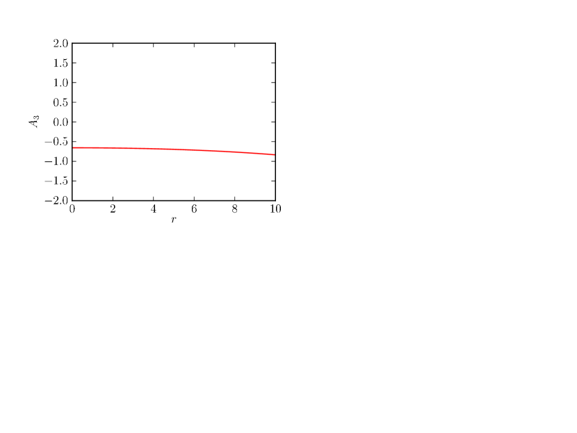
Figure 4: The plot of parameter $A_{3}$.

To obtain an expression for parameter $A_{3}$, one has to evaluate $\langle m_{j}\rangle$’s and $\langle\mu_{j}\rangle$’s, $j=1,2,3,4$, with respect to the nonlinear squeezed states $|\beta,\tilde{f}\rangle$. Let us first calculate $\langle m_{j}\rangle$:

$$\qquad\qquad m_{j}|\beta,\tilde{f}\rangle=N_{\beta}\sum^{\infty}_{n=0}\frac{\beta^{n}}{2^{n}n!}\sqrt{\frac{(2n)!}{(2n+2)!\;(2n+3)!}}\;m_{j}|2n+3\rangle.$$ (43)

Since $m_{j}|2n+3\rangle=K^{j}_{+}K^{j}_{-}|2n+3\rangle=2n(2n-1)(2n-2)...(2n-j+1)|2n+3\rangle$, we get

$$\qquad\qquad m_{j}|\beta,\tilde{f}\rangle=N_{\beta}\sum^{\infty}_{n=0}\frac{\beta^{n}}{2^{n}\;n!}\sqrt{\frac{(2n)!}{\;(2n+2)!\;(2n+3)!}}$$

$$\qquad\qquad\qquad\qquad\times\;2n(2n-1)...(2n-j+1)\;|2n+3\rangle.$$ (44)

Using (44), we find

$$\qquad\qquad\langle\beta,\tilde{f}|m_{j}|\beta,\tilde{f}\rangle=N^{2}_{\beta}\sum^{\infty}_{n=\lceil\frac{j}{2}\rceil}\frac{|\beta|^{2n}\;((2n)!)^{2}}{(2n-j)!4^{n}(n!)^{2}\;(2n+2)!\;(2n+3)!},$$ (45)

where $\lceil\frac{j}{2}\rceil$ is ceiling($\frac{j}{2}$). Using these expressions, we calculate parameter $A_{3}$ for the nonlinear squeezed states $|\beta,\tilde{f}\rangle$. The result is given in figure 4. The figure confirms that the value of parameter $A_{3}$ lies in between $-1$ and $0$ for all positive values of $r$. The negative values prove the non-classical nature of the nonlinear squeezed states.

4.3 Quadrature squeezing

To study the non-classical nature of the squeezed states, we define two Hermitian operators, namely $\hat{x}$ and $\hat{p}$ in terms of the deformed creation and annihilation operators, $\hat{K}_{+}$ and $\hat{K}_{-}$ in the form [17, 19, 20]

$$\hat{x}=\frac{1}{\sqrt{2}}(\hat{K}_{+}+\hat{K}_{-}),\qquad\hat{p}=\frac{i}{\sqrt{2}}(\hat{K}_{+}-\hat{K}_{-}).$$ (46)

The operators $\hat{x}$ and $\hat{p}$ satisfy the commutation relation $[\hat{x},\hat{p}]=i$.

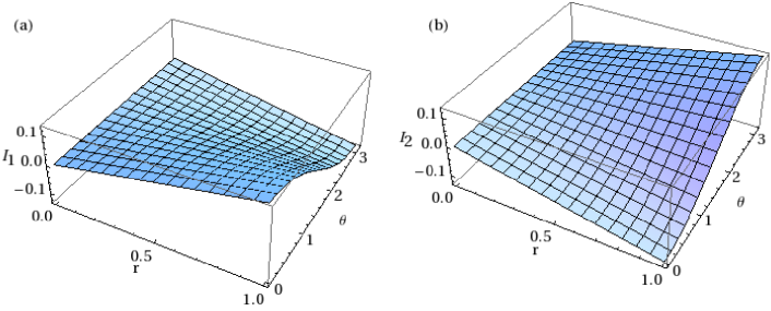
Figure 5: The plots of the identities (a) $I_{1}$ and (b) $I_{2}$ calculated with respect to nonlinear squeezed states (29) with $n_{max}=70$.

The squeezed states (29) and (34) satisfy the Heisenberg uncertainty relation $(\Delta\hat{x})^{2}(\Delta\hat{p})^{2}\geq\frac{1}{4}$ . A state is said to be squeezed in $\hat{x}$ or $\hat{p}$, if $(\Delta\hat{x})^{2}<\frac{1}{2}$ or $(\Delta\hat{p})^{2}<\frac{1}{2}$. Here, $\Delta\hat{x}$ and $\Delta\hat{p}$ denote the uncertainties in $\hat{x}$ and $\hat{p}$ respectively. The squeezing conditions can be transformed to the forms [40]

$$\qquad I_{1} = \langle\hat{K}^{2}_{-}\rangle+\langle\hat{K}^{2}_{+}\rangle-\langle\hat{K}_{-}\rangle^{2}-\langle\hat{K}_{+}\rangle^{2}-2\langle\hat{K}_{-}\rangle\langle\hat{K}_{+}\rangle+2\langle\hat{K}_{+}\hat{K}_{-}\rangle<0,$$ (47)

$$\qquad I_{2} = -\langle\hat{K}^{2}_{-}\rangle-\langle\hat{K}^{2}_{+}\rangle+\langle\hat{K}_{-}\rangle^{2}+\langle\hat{K}_{+}\rangle^{2}-2\langle\hat{K}_{-}\rangle\langle\hat{K}_{+}\rangle+2\langle\hat{K}_{+}\hat{K}_{-}\rangle<0,$$ (48)

where the expectation values are to be calculated with respect to squeezed states for which the quadrature squeezing has to be examined.

The identities, (47) and (48), are calculated for the nonlinear squeezed states (29) and presented in figures 5(a) and 5(b) respectively with $\beta=re^{i\;\theta}$.

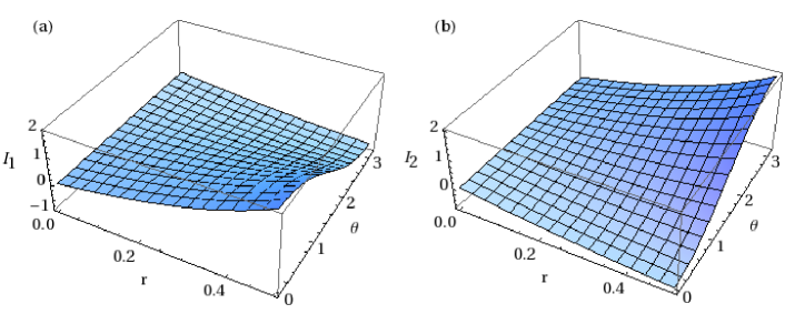
Figure 6: The plots of the identities (a) $I_{1}$ and (b) $I_{2}$ calculated with respect to squeezed states (34) with $n_{max}=70$.

From figures 5(a) and 5(b), we observe that the identities (47) and (48) for the nonlinear squeezed states $|\beta,\tilde{f}\rangle$ satisfying the uncertainty relation show small oscillations in $I_{1}$ and $I_{2}$. These two quantities, $I_{1}$ and $I_{2}$, oscillate out of phase $\pi$ with each other. In other words the squeezing can be observed in both the quadratures, $\hat{x}$ and $\hat{p}$, at different values of $\theta$.

The same type of squeezing is observed in the squeezed states (34) as well, which is depicted in figures 6(a) and 6(b). The squeezing shown by the nonlinear squeezed states (29) and squeezed states (34) confirm the non-classical nature of the associated states.

4.4 Amplitude-squared squeezing

The amplitude-squared squeezing, which was introduced by Hillery [41], involves two operators which represent the real and imaginary parts of the square of the amplitude of a radiation field. To investigate the amplitude-squared squeezing effect, we introduce again two Hermitian operators $\hat{X}$ and $\hat{P}$ from $\hat{K}_{+}$ and $\hat{K}_{-}$ respectively of the form

$$\hat{X}=\frac{1}{\sqrt{2}}(\hat{K}^{2}_{+}+\hat{K}^{2}_{-}),\qquad\hat{P}=\frac{i}{\sqrt{2}}(\hat{K}^{2}_{+}-\hat{K}^{2}_{-}).$$ (49)

Here $\hat{X}$ and $\hat{P}$ are the operators corresponding to the real and imaginary parts of the square of the complex amplitude of a radiation field. The Heisenberg uncertainty relation of these conjugate operators is then given by $(\Delta\hat{X})^{2}(\Delta\hat{P})^{2}\geq-\frac{1}{4}\langle[\hat{X},\hat{P}]\rangle^{2}$. For the nonlinear squeezed states (29) and the squeezed states (34), we find $(\Delta\hat{X})^{2}<-\frac{i}{2}\langle[\hat{X},\hat{P}]\rangle$ or $(\Delta\hat{P})^{2}<-\frac{i}{2}\langle[\hat{X},\hat{P}]\rangle$ which in turn confirm that the states are non-classical. The conditions for the amplitude-squared squeezing read [40]

$$\qquad I_{3}=\frac{1}{4}\left(\langle{\hat{K}_{-}}^{4}\rangle+\langle{\hat{K}_{+}}^{4}\rangle-\langle{\hat{K}_{-}}^{2}\rangle^{2}-\langle{\hat{K}_{+}}^{2}\rangle^{2}-2\langle{\hat{K}_{-}}^{2}\rangle\langle{\hat{K}_{+}}^{2}\rangle+\langle{\hat{K}_{+}}^{2}{\hat{K}_{-}}^{2}\rangle+\langle{\hat{K}_{-}}^{2}{\hat{K}_{+}}^{2}\rangle\right)$$

$$-\langle{\hat{K}_{+}}{\hat{K}_{-}}\rangle-\frac{1}{2}<0,$$ (50)

$$\qquad I_{4}=\frac{1}{4}\left(-\langle{\hat{K}_{-}}^{4}\rangle-\langle{\hat{K}_{+}}^{4}\rangle+\langle{\hat{K}_{-}}^{2}\rangle^{2}+\langle{\hat{K}_{+}}^{2}\rangle^{2}-2\langle{\hat{K}_{-}}^{2}\rangle\langle{\hat{K}_{+}}^{2}\rangle+\langle{\hat{K}_{+}}^{2}{\hat{K}_{-}}^{2}\rangle+\langle{\hat{K}_{-}}^{2}{\hat{K}_{+}}^{2}\rangle\right)$$

$$-\langle{\hat{K}_{+}}{\hat{K}_{-}}\rangle-\frac{1}{2}<0,$$ (51)

where the expectation values are to be calculated with respect to the nonlinear squeezed states $|\beta,\tilde{f}\rangle$ for which the amplitude-squared squeezing property has to be examined.

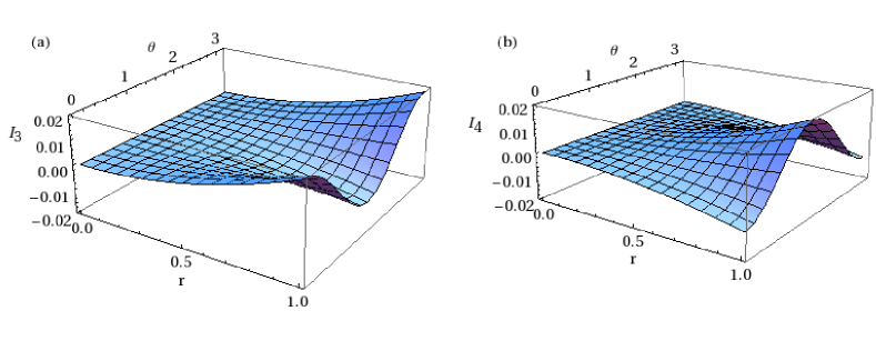
Figure 7: The plots of the identities (a) $I_{3}$, and (b) $I_{4}$ calculated with respect to nonlinear squeezed states (29) for $n_{max}=70$.

We evaluate the identities, (50) and (51), numerically and plot the results in figures 7(a) and 7(b). The identities $I_{3}$ and $I_{4}$ also vary in an oscillatory manner. For certain values of $r$ and $\theta$ when one of the identities $I_{3}\;($or $I_{4})$ is positive the other identity $I_{4}\;($or $I_{3})$ becomes negative. The negativity of $I_{3}\;(I_{4})$ indicates the amplitude squared squeezing in $\hat{X}\;(\hat{P})$ operators respectively.

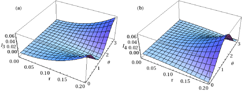
Figure 8: The plots of the identities (a) $I_{3}$, and (b) $I_{4}$ calculated with respect to squeezed states (34).

We calculate the identities $I_{3}$ and $I_{4}$ in (50) and (51) for the squeezed states (34) and plot the results in figure 8(a) and 8(b), which in turn confirm the non-classical nature of the squeezed states.

5 Quadrature distribution and quasi-probability distribution functions

5.1 Phase-parameterized field strength distribution

We study phase-parameterized distribution for the nonlinear squeezed states $|\beta,\tilde{f}\rangle$, in order to analyze the nature of the dependency of quantum noise on phase, which is defined to be [42]

$$P(x,\phi)=|\langle x,\phi{|\beta,\tilde{f}\rangle}|^{2},$$ (52)

where $|x,\phi\rangle$ is the eigenstate of the quadrature component $\hat{x}(\phi)=\frac{1}{\sqrt{2}}\left(e^{-i\phi}\hat{K}_{-}+e^{i\phi}\hat{K}_{+}\right)$. In other words

$$\hat{x}(\phi)|x,\phi\rangle=x|x,\phi\rangle,$$ (53)

which can be expressed in photon number basis in the form

$$|x,\phi\rangle=\frac{e^{\frac{-x^{2}}{2}}}{\pi^{\frac{1}{4}}}\sum^{\infty}_{n=0}\frac{H_{n}(x)e^{in\phi}}{\sqrt{2^{n}n!}}|n+3\rangle,$$ (54)

where $H_{n}(x)$ is the Hermite polynomial. Substituting (54) in (52) with $\beta=re^{i\theta}$ we obtain

$$\quad P(x,\phi)=\frac{{N}^{2}_{\beta}e^{-x^{2}}}{\sqrt{\pi}}\sum^{\infty}_{n,m=0}\left(\frac{r}{4}\right)^{n+m}\frac{H_{2n}(x)H_{2m}(x)}{n!\;m!}$$

$$\quad\qquad\quad\times\frac{\cos[(m-n)(2\phi-\theta)]}{\sqrt{(2n+2)!\;(2m+2)!\;(2n+3)!\;(2m+3)!}}.$$ (55)

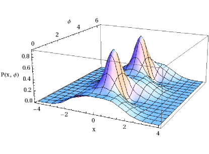
Figure 9: The plot of $P(x,\phi)$ which is calculated with respect to squeezed states (29)

From the expressions (55), we determine the quadrature function numerically with $\beta=re^{i\theta}$. The numerical results are displayed in figure 9 with $r=10$ and $\theta=0.5$ for the nonlinear squeezed states $|\beta,\tilde{f}\rangle$. The figure 9 shows an oscillating wave packet around $x=0$ with two peaks near $\phi=\frac{\pi}{2}$ and $\frac{3\pi}{2}$. When $|x|>3$, the phase information $P(x,\;\phi)$ disappears. The quadrature distribution $P(x,\;\phi)$ plotted in figure 9 depicts the time evolution of position probability density of the squeezed vacuum state during one oscillation period. In fact, this quadrature distribution plot matches with the experimental result reported in Ref. [43].

5.2 $s$-parameterized quasi-probability function

In this sub-section, we study $s$-parameterized quasi-probability distribution function for the nonlinear squeezed states (29). The $s$-parameterized quasi-probability distribution function is defined as the Fourier transform of the $s$-parameterized characteristic function [44, 45, 46]

$$F(z,s)=\frac{1}{\pi^{2}}\int C(\lambda,s)e^{(\lambda^{*}z-\lambda z^{*})}d^{2}\lambda,$$ (56)

where

$$C(\lambda,s)=\mbox{Tr}[\hat{\rho}D(\lambda)]\exp{\left[\frac{s}{2}|\lambda|^{2}\right]}$$ (57)

is the $s$-parameterized characteristic function [42] and $D(\lambda)$ is the displacement operator. To study the quasi-probability distribution for the nonlinear squeezed states constructed for the system (1), we consider the unitary displacement operator $D(\lambda)=\exp{(\lambda\hat{K}_{+}-\lambda^{*}\hat{K}_{-})}$ from Case (iii) since $\hat{K}_{-}$ and $\hat{K}_{+}$ act as annihilation and creation operators $\hat{a}$ and $\hat{a}^{\dagger}$. This $s$-parameterized function is introduced by Cachill and Glauber with $s$ being a continuous variable [44]. This function is known as the generalized function that interpolates the Glauber-Sudarhsan $P$-function for $s$ = 1, Wigner function $W$ for $s=0$ and Husimi $Q$-function for $s=-1$ [44]. The quasi-probability distribution functions provides insight into the non-classical features of the radiation field.

The characteristic function (57) for the squeezed states read

$$C(\lambda,s)=\exp{\left[\frac{s}{2}|\lambda|^{2}\right]}\sum^{\infty}_{m,\;n=0}{B}_{n,\;m}\langle 2m+3|D(\lambda)|2n+3\rangle,$$ (58)

where the coefficients ${B}_{n,\;m}$ for the nonlinear squeezed states $|\beta,\tilde{f}\rangle$ are

$$\quad\quad{B}_{n,\;m}=N^{2}_{\beta}\sum^{\infty}_{n,m=0}\frac{{\beta^{*}}^{m}\beta^{n}}{2^{n+m}\;n!\;m!}\sqrt{\frac{(2n)!\;(2m)!}{(2n+2)!\;(2m+2)!\;(2n+3)!\;(2m+3)!}}.$$ (59)

To evaluate $C(\lambda,s)$, one can derive the expression for $\langle 2m+3|D(\lambda)|2n+3\rangle$ as, [44, 46]

$$\langle 2m+3|D(\lambda)|2n+3\rangle = e^{-\frac{|\lambda|^{2}}{2}}\sqrt{\frac{(2n)!}{(2m)!}}{\lambda^{*}}^{2n-2m}L^{2n-2m}_{2m}(|\lambda|^{2}).$$ (60)

where $L^{2n-2m}_{2m}(|\lambda|^{2})$ is an associated Laguerre polynomials [47].

Using the expectation value (60) in (58) and then substituting the resultant expression in (56), we arrive at

$$F(z,s)=\frac{1}{\pi^{2}}\sum^{\infty}_{n,m=0}{B}_{n,\;m}\sqrt{\frac{(2n)!}{(2m)!}}\int\exp{\left[\frac{(s-1)}{2}|\lambda|^{2}+\lambda^{*}z-\lambda z^{*}\right]}$$

$$\qquad\qquad\quad\qquad\times{(\lambda^{*})}^{2n-2m}L^{2n-2m}_{2m}(|\lambda|^{2})d^{2}\lambda.\;\;\;$$ (61)

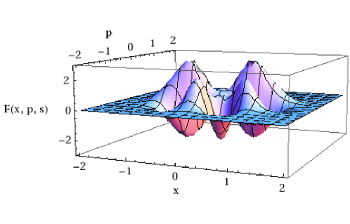
Figure 10: The plot of $s$-parameterized quasi probability distribution function corresponding to nonlinear squeezed states (29) for $s=0.5$.

Evaluating the integral in (61), we find

$$\quad F(z,s)=\frac{2\exp{\left[\frac{2}{(s-1)}|z|^{2}\right]}}{\pi(1-s)}\sum^{\infty}_{n,m=0}{B}_{n,\;m}{(2z^{*})}^{2n-2m}\sqrt{\frac{(2n)!}{(2m)!}}\frac{(s+1)^{2m}}{(s-1)^{2n}}$$

$$\qquad\qquad\quad\qquad\times L^{2n-2m}_{2m}\left(\frac{4}{(1-s^{2})}|z|^{2}\right),$$ (62)

where $L^{2n-2m}_{2m}(|\lambda|^{2})$ is an associated Laguerre polynomial.

We consider the value $s$ in-between $0$ and $1$ and calculate a general quasi-probability distribution function instead of investigating the special cases one by one, that is (i) $s=1$ (Glauber-Sudarshan $P$-function), (ii) $s=0$ (Wigner function $W$) and (iii) $s=-1$ (Husimi $Q$-function). Using (59) in (62), we numerically calculate $s$-parameterized quasi-probability distribution function, with $s=0.5$ for the nonlinear squeezed states $|\beta,\tilde{f}\rangle$ (with $\beta=2+i2$) and display the results in figure 10 with $z=x+i\;p$. The function $F(x,p,s)$ has negative values for the nonlinear squeezed states $|\beta,\tilde{f}\rangle$. The results reveal the non-classical nature of the nonlinear squeezed states.

6 Conclusion

In this paper, we have constructed nonlinear squeezed states for the generalized isotonic oscillator by transforming the deformed ladder operators, which satisfy the deformed oscillator algebra, suitably in such a way that they produce the Heisenberg algebra. We observed that the transformation can be made in three different ways. While implementing this we obtain non-unitary squeezing operator in two cases and an unitary squeezing operator in the third case. One of the two non-unitary squeezing operators produces the nonlinear squeezed states whereas the other one fails to produce their dual pair. The unitary squeezing operator produces squeezed states only. The non-classical nature of the nonlinear squeezed states has been confirmed through the evaluation of photon number distribution, Mandel’s parameter, second-order correlation function and parameter $A_{3}$. Further, we have demonstrated that the nonlinear squeezed states possess other non-classical properties as well, namely quadrature and amplitude-squared squeezing. We have also analyzed the quadrature distribution and $s$-parameterized quasi-probability function for the nonlinear squeezed states which again confirmed the non-classical nature of these states. The results summarized in this paper are all useful in the quantum entanglement perspective.

References

References

- [1] Cariñena J F, Perelomov A M, Rañada M F and Santander M 2008 J. Phys. A: Math. Theor. 41 085301
- [2] Fellows J M and Smith R A 2009 J. Phys. A: Math. Theor. 42 335303
- [3] Berger M S and Ussembayev N S 2010 Phys. Rev. A 82 022121
- [4] Sesma J 2010 J. Phys. A: Math. Theor. 43 185303
- [5] Hall R L, Saad N and Özlem Yeşiltaş 2010 J. Phys. A: Math. Theor. 43 465304
- [6] Sadd N, Hall R L, Çiftçi H and Özlem Yeşiltaş 2011 Adv. Math. Phys. 2011 750168
- [7] Kraenkel R A and Senthilvelan M 2009 J. Phys. A: Math. Theor. 42 415303
- [8] Chithiika Ruby V and Senthilvelan M 2010 J. Math. Phys. 51 052106
- [9] Chithiika Ruby V and Senthilvelan M 2010 J.Phys.A: Math. Theor. 43 415301
- [10] Junker G and Roy P 1997 Phys. Lett. A 232 155
- [11] Quesne C 2008 J. Phys. A: Math. Theor. 41 392001
- [12] de Matos Filho R L and Vogel W 1996 Phys. Rev. A 54 4560; Man’ko V I, Marmo G, Sudarshan E C G and Zaccaria F 1997 Phys. Scr. 55 528
- [13] Sunilkumar V, Bambah B A, Panigrahi P K and Srinivasan V 1999 Coherent states for the deformed algebras arXiv:quant-ph/9905010v1
- [14] Sklyanin E K 1982 Funct. Anal. Appl. 16 262
- [15] Delbecq C and Quesne C 1993 J. Phys. A: Math. Gen. 26 L127
- [16] Man’ko V I, Marmo G, Solimeno S and Zaccaria F 1993 Int. J. Mod. Phys. A 3577; Mizrahi S S, Camargo Lima J P and Dodonov V V 2004 J. Phys. A: Math. Gen. 37 3707
- [17] Walls D F and Zoller P 1981 Phys. Rev. Lett. 47 709; Walls D F 1983 Nature 306 141
- [18] Stoler D 1970 Phys. Rev. D 1 3217
- [19] Yuen H P 1976 Phys. Rev. A 13 2226
- [20] Hong C K and Mandel L 1985 Phys. Rev. Lett. 54 323
- [21] Darwish M 2007 Eur. Phys. J. D 41 547
- [22] Obada A-S F and Abd Al-Kader G M 2007 Eur. Phys. J. D 41 189; Obada A-S F 2011 J. Egypt. Math. Soc. doi:10.1016/j.joems.2011.09.013
- [23] Kwek L C and Kiang D 2003 J. Opt. B: Quantum Semiclass. Opt. 5 383; Darwish M 2005 Int. J. Mod. Phys. B 19 715; Kolesnikov A A and Manḱo V I 2008 J. Rus. Laser Research 29 142
- [24] Bennett C H, Brassard G, Mermin N D 1992 Phys. Rev. Lett. 68 557; Kempe J 1999 Phys. Rev. A 60 910
- [25] Wang X 2001 Phys. Rev. A 64 022302; An N B 2009 Phys. Lett. A 373 1701
- [26] Gross C, Zibold T, Nicklas E, Estéve and Oberthaler M K 2010 Nature 464 1165
- [27] Yuen P H and Shapiro H J 1979 Opt. Lett. 4 334; Reid M D and D. F. Walls D F 1985 Phys. Rev. A 31 1622
- [28] Shelby R M, Levenson M D, Perlmutter S M, DeVoe R G and Walls D F 1986 Phys. Rev. Lett. 57 691
- [29] Milburn G J and Walls D F 1981 Opt. Commun. 39 401; Collet M J and Gardiner C W 1984 Phys. Rev. A 30 1386; Wu L -A, Kimble H J, Hall J L and Wu H 1986 Phys. Rev. Lett. 57 2520; Heidmann A, Horowicz R J, Reynaud S, Giacobino E, Fabre C and Camy G 1987 Phys. Rev. Lett. 59 2555
- [30] Lugiato L A and Strini G 1982 Opt. Commun. 41 67; Collet M J and Walls D F 1985 Phys. Rev. A 32 2887
- [31] Roknizadeh R and Tavassoly M K 2005 J. Math. Phys. 46 042110; Roy B and Roy P 2000 J. Opt. B: Quantum Semicalss. Opt. 2 65
- [32] Chithiika Ruby V and Senthilvelan M 2011 J. Phys. A: Math. Theor. An observation of quadratic algebra, dual family of nonlinear coherent states and their non-classical properties, in the generalized isotonic oscillator (submitted for publication)
- [33] Gazeau J-P 2009 Coherent states in Quantum Physics (Weinheim: Wiley-VCH)
- [34] Mandel L 1979 Opt. Lett. 4 205
- [35] Paul H 1982 Rev. Mod. Phys. 54 1061
- [36] Mahran M H and Venkata Satyanarayana M 1986 Phys. Rev. A 34 640
- [37] Antoine J P, Gazeau J P, Monceau P, Klauder J R and Penson K A 2001 J. Math. Phys. 42 2349
- [38] Agarwal G S and Tara K 1992 Phys. Rev. A 46 485
- [39] Tavassoly M K 2010 Opt. Commun. 283 5081
- [40] Roknizadeh R and Tavassoly M K 2004 J. Phys. A: Math. Gen. 37 8111
- [41] Hillery M 1987 Phys. Rev. A 36 3796
- [42] Obada A-S F and Abd Al-Kader G M 2005 J. Opt. B: Quantum Semiclass. Opt. 7 S635
- [43] Breitenbach G, Schiller S and Mlynek J 1997 Nature 387 471
- [44] Cahill K E and Glauber R J 1969 Phys. Rev. 177 1857; Cahill K E and Glauber R J 1969 Phys. Rev. 177 1882
- [45] Vogel W and Welsch D-G 2006 Quantum Optics (Weinheim: Wiley-VCH)
- [46] Barnett S M and Radmore P M 1997 Methods in Theoretical Quantum Optics (Clarendon: Oxford University Press)
- [47] Gradshteyn I S and Ryzhik I M 1980 Table of Integrals, Series and Products (New York: Academic)