Modeling rhythmic patterns in the hippocampus

Abstract

We investigate different dynamical regimes of neuronal network in the CA3 area of the hippocampus. The proposed neuronal circuit includes two fast- and two slowly-spiking cells which are interconnected by means of dynamical synapses. On the individual level, each neuron is modeled by FitzHugh-Nagumo equations. Three basic rhythmic patterns are observed: gamma-rhythm in which the fast neurons are uniformly spiking, theta-rhythm in which the individual spikes are separated by quiet epochs, and theta/gamma rhythm with repeated patches of spikes. We analyze the influence of asymmetry of synaptic strengths on the synchronization in the network and demonstrate that strong asymmetry reduces the variety of available dynamical states. The model network exhibits multistability; this results in occurrence of hysteresis in dependence on the conductances of individual connections. We show that switching between different rhythmic patterns in the network depends on the degree of synchronization between the slow cells.

I Introduction

Rhythmic behavior is a basic property of biological systems and plays an important role in a variety of physiological processes Winfree . In particular, hippocampal neurons of the human brain are able to generate rhythmic oscillations in several frequency ranges; among these, prominent roles belong to fast (gamma-rhythm, 30$\div$65 Hz) and slow (theta-rhythm, 3$\div$10 Hz) signals and to mixed regimes in which fast and slow oscillations alternate. Theta-rhythm has been demonstrated to be responsible for coding of spatial information Keef , synaptic modification of intrahippocampal pathways, as well as for assembling and segregation of neuronal groups Bur . In its turn, oscillatory activity in the gamma-frequency band is involved in information transmission and storage Harr . Isolated parts (so-called CA1, CA3, DG etc.) of hippocampal formation where these regimes are observed, have been subjected to numerous experiments Haj ; Glov ; Gloveli ; Macca ; Mann ; Klaus . In particular, it has been established that the neuronal network in the CA3 region of the hippocampus can exhibit three qualitatively different oscillatory states (theta-, gamma- and the mixed “theta/gamma”) and is able to dynamically switch between them Gloveli . Transitions between different regimes in brain neuronal networks can be provoked not only by variation of parameters, but by variation of initial conditions as well Fro ; Durst ; Kass ; Sasaki ; the latter may occur due to changes in the baseline potential Kass or to perturbations of initial ionic concentrations Hahn .

Cells, which constitute a hippocampal network, differ in their morphological, electrophysiological and neurochemical properties Ander . Synaptic interactions between several types of cells: the pyramidal ones, basket, septum and oriens-lacunosum-moleculare (OLM) cells are responsible for the generation of different rhythms Klaus .

Besides experimental studies, transitions between various rhythms and multistability phenomena in isolated cells as well as in neuronal networks have been subjected to theoretical and numerical modeling Gloveli ; Kopell ; Siek ; Frohl ; Rab1 . Typically, such models involve various cell types as well as large numbers of ionic currents and compartments. In the detailed models Traub ; Frohl as well as in simpler biophysical approximations Kopell the cells, responsible for the generation of rhythmic patterns, are typically described by equations of the Hodgkin-Huxley type.

Role of intercellular synchronization in the transitional processes is an object of ongoing discussions. In particular, it has been shown Sing that a switching between two states of the system can forecast desynchronization in a bursting activity of the hippocampus. The strength of intercellular coupling governed by synaptic conductances is apparently a crucial factor in this context Gloveli ; Rab . For example, studies of detailed thalamocortical model Rab1 have shown that presence or absence of bistability in the neuronal circuit can depend on parameters of the electrical coupling between neurons as well as on the synaptic conductance.

High degree of complexity, obligatory in realistic models, hampers revealing of principal mechanisms and control parameters of transitions between different types of oscillations. Therefore, along with accurate reproduction of experimental observations, one of the main aims of the modeling remains a consideration of general dynamics in the appropriate class of circuits, as well as an understanding of the underlying dynamical mechanisms which are responsible for different rhythmic patterns. This raises a question about a minimal module of the hippocampal network: a small set of cells capable of reproducing all basic typs of experimentally observable rhythms Kopell . Embedded into intricate networks of neurons, such modules can play a role of pacemakers which ensure persistence of optimal oscillatory states in the entire ensemble.

Below we discuss a minimalistic dynamical model of the hippocampal circuit in the area CA3, which is able to produce several rhythmic patterns. For this purpose we simplify the basic module of the circuit in such a way that maintenance of the essential types of dynamical regimes would be controlled by a concise number of principal parameters. Since we do not aim at detailed reproduction of intrinsic cellular dynamics but restrict ourselves to rhythmic aspects, we reduce the description of each element to the classical simplified model of neuronal oscillations: the FitzHugh-Nagumo (FHN) equations. Simplification of elements in this case does not imply trivialization of dynamics: ensembles of the FHN oscillators are known to exhibit different kinds of collective behavior which, depending on the topology and strength of interaction, range from subthreshold oscillations via mixed-mode intermittency to tonic spiking zssgn . Interplay between connectivity and coupling strength in networks of heterogeneous FHN oscillators can induce or destroy synchrony hennig . Working with FHN neurons renders the well-understood dynamics on the level of individual elements and allows us to concentrate on the governing role of interactions between them.

In Sect. II we introduce the model equations and discuss the choice of appropriate parameter values. Sect. III begins with characterization of the principal rhythmic patterns; in particular, the role of the phase shift between the OLM cells is discussed. Further we proceed to the description of multistability and transitions between the patterns. We demonstrate that the model reproduces the basic rhythms observed experimentally, as well as hysteresis between them. Finally, we show how the symmetry or asymmetry in the arrangement of synaptic connections influences the existence and properties of dynamical states.

II Model equations

In a recent paper Gloveli , a kind of minimalistic network for studies of different regimes in the hippocampal area CA3 has been proposed. This network includes main types of hippocampal cells and consists of five elements: two fast-oscillating cells (so-called basket cells), two slow cells (OLM – oriens/lacunosum-moleculare associated – cells) and one two-compartmental pyramidal cell. The cells are synaptically connected in all-to-all topology, with one exception: there is no direct connection between the slowly spiking cells. Accordingly, the pyramidal cell activates the rest of the cells which, in turn, inhibit each other and the pyramidal cell. The cells are described within the framework of the Hodgkin-Huxley formalism. After taking into account all relevant currents as well as kinetics of synaptic variables, the resulting system constitutes a set of 41 ordinary differential equations. Notably, the choice of coupling coefficients employed in Gloveli ensured a certain degree of asymmetry in the network: in particular, each basket cell was coupled to both OLM-cells through connections with different conductivity.

Numerical simulations of that model have confirmed that transitions between different regimes depend on the strength of coupling between the cells. Typically, a switching between different rhythms is preceded by onset of a certain phase shift between two slow-spiking cells. Within the model of Gloveli , this shift can be ensured e.g. by a judicious choice of appropriate initial conditions.

In the present work we further reduce the complexity of the model: we decrease the number of cells and replace the Hodgkin-Huxley setup by the FitzHugh-Nagumo equations. The resulting network, sketched in Fig.1, includes one-compartmental pyramidal cell $P$, one basket cell $B$ and two OLM-cells $L_{1}$ and $L_{2}$. All cells are mutually synaptically connected; the only exception are two slow OLM-cells which do not communicate directly. Synaptic connections are governed by the synaptic conductances $G_{ji}$ with $j,i=L_{1},\,L_{2},\,P,\,B$ (and $G_{jj}$=0). Leaving in the network only one basket cell $B$, we take into account, however, inequality of the cross- and direct- connections as a potential source of a phase shift between the slowly spiking cells. For this purpose, it is sufficient to allow for asymmetric synaptic inputs from the basket cell to $L_{1}$ and $L_{2}$: in general, $G_{BL_{1}}\neq G_{BL_{2}}$. The rest of connections is set symmetrically: $G_{PL_{1}}$=$G_{PL_{2}}$=$G_{PL}$, $G_{L_{1}P}$=$G_{L_{2}P}$=$G_{LP}$, $G_{L_{1}B}$=$G_{L_{2}B}$=$G_{LB}$.

Within this simplified description, it appears reasonable to keep only one activating input which acts upon the fast-oscillating cell $P$. The latter excites all other cells, which inhibit each other as well as $P$ itself.

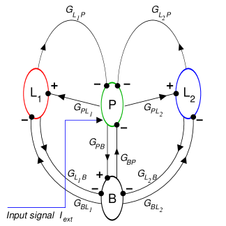
Figure 1: (Color Online). Sketch of the cellular network. $L_{1,2}$: slow OLM cells; $P$: fast pyramidal cell; $B$: basket cell. Arrows: directions of currents. Filled circles: synapses. Pluses: excitatory synapses; minuses: inhibitory synapses. Synaptic connections are characterized by conductances $G_{ji}$. External input $I_{ext}$ affects only the pyramidal cell $P$.

We use below the form of equations in which all variables, and, hence, all parameters are measured in dimensionless units. Each cell of the network obeys the standard set of coupled FitzHugh-Nagumo equations:

$$\frac{dv_{i}}{dt} = v_{i}-\frac{v_{i}^{3}}{3}-u_{i}+I_{\rm ext}\delta_{i,P}+\sum_{j}I_{\rm syn}^{(ji)},$$

$$\frac{du_{i}}{dt} = \varepsilon_{i}\,(v_{i}+a-b\,u_{i}).$$

where $v_{i}$ is the membrane potential of the $i$-th cell (recall that $i=L_{1},L_{2},P,B$), and $u_{i}$ is the respective membrane variable. The values of parameters $a$ and $b$ are the same for all cells. The Kronecker-delta $\delta_{i,P}$ ensures that only the pyramidal cell is externally excited by the current $I_{\rm ext}$.

The synaptic input $I_{\rm syn}^{(ji)}$ in Eqs (LABEL:equations) – the current from cell $j$ to cell $i$ – is defined as

$$I_{\rm syn}^{(ji)}=G_{ji}s_{ji}\,(E_{\rm ex,in}-v_{i})$$

and is governed by kinetic equation for the synaptic variable $s_{ji}(t)$ Kopell :

$$\frac{ds_{ji}}{dt}=\frac{A}{2}\left(1+\tanh\frac{v_{j}}{v_{vsl}}\right)(1-s_{ji})-Bs_{ji},$$ (2)

For simplicity, we assume that all synapses obey quantitatively the same kinetics. This is achieved by using the same values of $A$, $B$ and $v_{vsl}$ in (2) for all $s_{ji}$. Hence, evolution of $s_{ji}$ depends (via $v_{j}$) only on $j$, and the number of independent synaptic variables equals the number of cells in the network. Altogether, the dynamical system includes 12 ordinary differential equations: 8 equations for the FitzHugh-Nagumo variables along with 4 equations for the synaptic variables.

Originally, the FitzHugh-Nagumo equations were written as a crude simplistic model which mimics the characteristic features of the Hodgkin-Huxley dynamics. Hence, their parameters do not allow for direct biological interpretation and serve the mere purpose of supporting the proper dynamical regimes. To illustrate possible kinds of dynamics in the considered network, we fix the parameters of the FitzHugh-Nagumo equations (LABEL:equations) at the values which ensure that in absence of external currents every isolated cell is at rest; if perturbed by sufficient external input, it displays full-scale oscillations. The values $a$=0.5, $b$=0.8 which we use for our calculations, are close to those employed by FitzHugh FH_69 .

The parameter $\varepsilon_{i}$ in the FitzHugh-Nagumo equations (LABEL:equations) determines the timescale of oscillations in the isolated $i$-th cell: in the leading order, period of relaxation oscillations in a cell is inversely proportional to $\varepsilon_{i}$. The dimensionless number $\varepsilon_{i}$ can be interpreted as ratio of two dimensional timescales of the neuron: that of the fastest relaxation to that of the slowest one. In the case of the pyramidal and the basket cells these are the relaxation times of, respectively, potassium and sodium currents; the values of $\varepsilon_{i}$ for these two cells can be viewed as (approximately) the same. In contrast, in the OLM-cells the slowest processes involve relaxation of specific so-called hyperpolarization-activated currents Macca ; Gil , and their values of $\varepsilon_{i}$ should be chosen substantially lower. Accordingly, we set $\varepsilon$=0.3 for the fast basket and pyramidal cells, whereas for slow $L$-cells the value $\varepsilon$=0.04 is adopted.

Equations (2) for synaptic variables are phenomenological as well; the values of parameters $A$, $B$ and $v_{vsl}$ are commonly obtained by fitting the experimentally measured dependencies. By setting $A$=1, $B$=0.3 and $v_{vsl}$=0.1 we model the typical situation in which opening of channels occurs faster – but not much faster – than their subsequent closure.

The value of $E$ in the expression for synaptic current depends on the kind of connection. For all excitatory synapses we put $E_{\rm ex}=0$, whereas for inhibitory synapses $E_{\rm in}$=–5 is set. The latter value ensures that the difference $E_{\rm in}-v_{i}$, and thereby the corresponding synaptic current $I_{\rm syn}^{(ji)}$ stay negative at all times, and the connection is indeed inhibitory.

Concerning synaptic conductances $G_{ji}$, we choose the values which, dimensionalized in units of 0.01$Ohm^{-1}m^{-2}$, have the order of magnitude of those, reported in Gloveli . In a sense, conductances predetermine the relative importance of individual cells in the ensemble. Since external current acts only upon the pyramidal cell, synaptic connections from this cell to the rest of the module should be strong enough in order to activate the otherwise silent basket and OLM-cells; this is ensured by assigning to them relatively high values $G_{PL}=0.7$ and $G_{PB}=0.57$. A lower conductivity is assigned to the backward connection from the basket to the pyramidal cell: $G_{BP}$=0.1. Further, we introduce asymmetry between the left and right halves of the network by fixing different values for connections from the basket to the OLM-cells: $G_{BL_{1}}$=0.06 in contrast to $G_{BL_{2}}$=0.03.

The slow OLM-cells are driven by the pyramidal cell; intensity of their inhibitory feedback to the driving element depends on conductances $G_{LP}$ and (mediated by the basket cell) on conductances $G_{LB}$. If both $G_{LB}$ and $G_{LP}$ are set to zero, the feedback is absent, and the OLM-cells play the passive role. Each of them oscillates periodically: it is phase-locked to the oscillations of the driving fast subsystem formed by the pyramidal cell and the basket cell. However, due to asymmetry, the slow cells can be locked (and under the quoted parameter values are indeed locked) to the fast subsystem in different locking ratios. Asymmetry of rhythmic patterns persists for sufficiently low values of $G_{LB}$ and $G_{LP}$: this is visualized in the lower panel of Fig.2 where the slow cells oscillate in the ratio 2:3. Increase of conductances $G_{LB}$ and/or $G_{LP}$ intensifies the feedback; in spite of the absence of the direct connection, the OLM-cells interact through the mediation of the fast cells, and their periods get adjusted.

In order to concentrate on the role of connection from the OLM-cells to the pyramidal cell, we use throughout this work the conductance $G_{LP}$ as a controlling parameter and study transitions which occur in the course of its variation. As for the connection from the OLM to the basket cell, it should be weak enough in order not to damp the module dynamics, hence we fix for our calculations (with the only exception of the plot in Fig.2) the value $G_{LB}=0.01$. This value is sufficiently high to ensure that the feedback via the basket cell synchronizes the slow cells in the frequency ratio 1:1, even in the absence of direct feedback through the $LP$-connections.

The steady solution of equations corresponds to the quiescent non-spiking state. Intensity of the constant external input $I_{\rm ext}$ (recall: it affects only the $P$-cell) should ensure destabilization of the equilibrium and sustainment of oscillations in the system. Under $G_{LP}$=0.037 and the aforementioned fixed values of other parameters, the equilibrium is unstable for $0.02<I_{\rm ext}<1.1$. In the endpoints of this interval, subcritical Hopf bifurcations take place. Location of the endpoints is almost insensitive to variation of $G_{LP}$. Accordingly, for our numerical simulations we take the value of input from this range: $I_{\rm ext}=0.43$.

Numerical solutions have been obtained using the software packages XPPAUT and MATCONT.

III Results

In order to characterize different attractors of the system and to understand possible mechanisms of switching between the regimes, we have studied the response of the model to variation of the strength of $LP$ connection. Starting from the situation when this connection is absent, we describe below the states which are observed in the course of increase of $G_{LP}$.

Among the solutions, we single out the three main qualitative types of oscillations. The difference between them lies in the behavior of the voltage variables of fast (pyramidal or basket) neurons: in the gamma-rhythm the voltage exhibits fast regular oscillations, whose amplitude is weakly modulated due to interaction with slow counterparts. In the theta/gamma rhythm certain spikes in the pattern “fall out”; the plot shows regular patches of spikes interrupted by nearly quiescent epochs. Typically, theta/gamma oscillations are periodic. Finally, the theta pattern consists of repeated solitary spikes on the nearly quiescent background. For a slow OLM-cell the difference in the temporal dynamics between three rhythms is not so pronounced; here, transitions manifest themselves in the onset or the disappearance of a phase shift between two such cells.

III.1 Gamma-rhythm

If the value of conductance $G_{LP}$ is set to zero, the OLM-cells exert no inhibiting action upon the pyramidal cell; this corresponds to removal of the upper connecting arcs in the scheme of Fig.1. In this situation, the system performs periodic oscillations of the gamma type. Consecutive spikes in the fast cells occur at close time intervals, but the exact repetition (in other words, closure of the limit cycle in the phase space of the system) requires several spikes. In particular, smallness of $G_{LB}$ can result in asynchrony between the slow cells (Fig. 2).

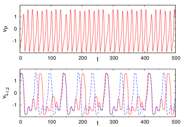
Figure 2: (Color Online). Gamma-rhythm at $G_{LP}$=0.032, $G_{LB}$=0.001. Top: pyramidal cell; periodic pattern which consists of 9 spikes. Bottom row: OLM cells; solid curve: $L_{1}$; dashed curve: $L_{2}$. OLM cells are locked in the frequency ratio 2:3.

By continuity, rhythmic pattern of the gamma type persists at sufficiently low non-zero values of $G_{LP}$ as well. An example is shown in Fig.3. At $G_{LP}=0.035$ the slow cells oscillate in the ratio $1:1$ (bottom panel), but their maxima do not occur simultaneously. In this context it is natural to speak about the phase shift. We introduce the phase phenomenologically: for each cell the phase increment of $2\pi$ is assigned to every interval between two consecutive positive maxima of voltage; between the maxima, the phase is linearly interpolated. The phase shift between oscillations shown in the bottom panel of Fig. 3 is close to $2\pi/3$.

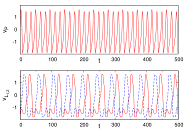
Figure 3: (Color Online). Gamma-rhythm at $G_{LP}$=0.035, $G_{LB}$=0.01. Top: pyramidal cell. Bottom row: OLM cells; solid curve: $L_{1}$; dashed curve: $L_{2}$. OLM-cells are locked in 1:1 ratio; note phase shift between them.

III.2 Theta/gamma rhythm

In a broad range of values $G_{LP}$ above 0.0362 an appropriate choice of initial condition results in a different rhythmic pattern: the system exhibits theta/gamma oscillations. The bottom panel of Fig. 4 indicates that in the theta/gamma state both slow cells oscillate synchronously; there is no phase shift between them.

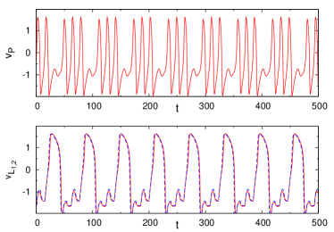
Figure 4: (Color Online). Theta/gamma-rhythm close to its onset; $G_{LP}$=0.05. Top: pyramidal cell. Bottom: OLM cells; solid curve: $L_{1}$; dashed curve: $L_{2}$.

III.3 Theta-rhythm

At sufficiently high values of $G_{LP}$ theta/gamma rhythm is replaced by theta-oscillations. Switching between the two regimes is visualized in Fig. 5: the motion starts as a typical theta/gamma oscillation, with patches of spikes of the fast cell; in the course of time evolution, at around $t\approx 200$, it abruptly changes the pattern and acquires the characteristic shape of theta rhythm with equidistant solitary spikes of the fast cell. Remarkably, the slow cells, synchronous on the initial stage, develop during the switch the phase shift of $\pi$: in the theta-rhythm the OLM cells oscillate in antiphase.

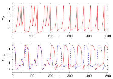
Figure 5: (Color Online). Breakdown of theta/gamma rhythm and onset of theta rhythm, $G_{LP}$=2.274. Top: pyramidal cell. Bottom: OLM cells; solid curve: $L_{1}$; dashed curve: $L_{2}$. Note in-phase oscillations before the switch and antiphase immediately after it.

III.4 Hysteresis

Over large intervals of values of $G_{LP}$, different rhythmic patterns coexist as attractors of Eqs (LABEL:equations,2): at low values of $G_{LP}$, depending on the initial values of the variables, the system can exhibit gamma- as well as theta/gamma-oscillations, whereas at moderate and high values of $G_{LP}$ there is a hysteresis between theta/gamma- and pure theta- patterns.

For slow OLM cells, neither a transition between gamma- and theta/gamma-states, nor the further growth of $G_{LP}$ significantly affect the period of their oscillations. In contrast, periodicity in spiking patterns of the fast cells $P$ and $B$ changes quite noticeably. A convenient characteristics is delivered by the average duration of interspike interval (ISI): the mean distance between the positive maxima of voltage in a cell. In Fig. 6, we plot this characteristics for membrane potential oscillations in the pyramidal cell. The value of ISI increases from 14.73 in the gamma state at $G_{LP}=0$ to 35.94 in the theta state at $G_{LP}=3$. Similar situation is observed for the basket cell.

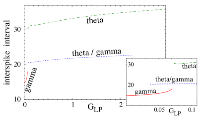
Figure 6: (Color Online). Duration of interspike intervals in dependence on $G_{LP}$ for different rhythmic patterns. Solid line: gamma-rhythm. Dotted line: theta/gamma pattern. Dashed line: theta rhythm. Inlet: range of low values of the conductance $G_{LP}$.

A closer look shows that gamma- and theta- branches are connected; in fact, they belong to the same continuous family of solutions. A transformation from the gamma- to theta-rhythm occurs through the intermediate regime which is observed within the small parameter range $0.0724<G_{LP}<0.0734$. Main stages of this process, in terms of the voltage variable of the pyramidal cell, are presented in Fig. 7. The transformation is preceded by a gradual deformation of the gamma-pattern: of the three initially nearly equal spikes (cf. Fig. 3), two spikes get diminished (Fig. 7(a,b)). As a result, the periodic gamma-state acquires the characteristic shape of mixed-mode oscillations Chaos_focus with alternating small subthreshold - and large-scale spiking maxima. At $G_{LP}=0.0726$ these oscillations form the complicated (yet periodic, with period 541.1 !) temporal pattern, visualized in Fig. 7(c). A small increase of $G_{LP}$ leads to partial flattening of subthreshold epochs (Fig. 7(d)); the next small increment results in the regular alteration of a spike and a single subthreshold oscillation (Fig. 7(e)). In fact, this state is already very close to the theta-pattern; further increase of $G_{LP}$ brings only quantitative changes: the subthreshold oscillations are gradually flattened, eliminated, and the theta state is established. On the phase portrait (cf. Fig. 8), the epochs of subthreshold oscillations are represented by minor loops of the trajectory. In the course of flattening, these loops get smaller, turn into cusps and disappear, so that only the large loops (corresponding to solitary spikes of the theta-rhythm) persist.

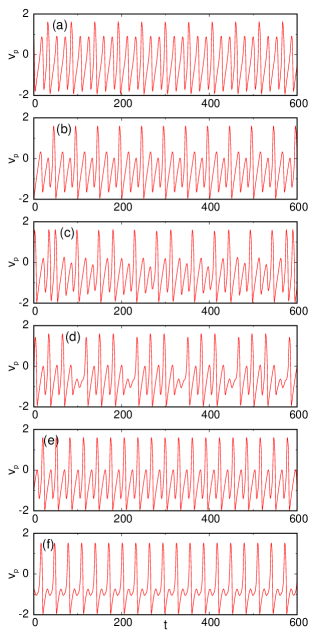
Figure 7: (Color Online). Transformation of gamma- into the theta-rhythm for the membrane voltage of the pyramidal cell. (a) $G_{LP}$=0.07; (b) $G_{LP}$=0.0724; (c) $G_{LP}$=0.0726; (d) $G_{LP}$=0.0732; (e) $G_{LP}$=0.0734; (f) $G_{LP}$=0.1000.

Remarkably, the described transformation changes the phase difference between the slow cells: as already mentioned, in the gamma-state the difference is close to $2\pi/3$, and the proximity to this value holds until the onset of mixed-mode oscillations in Fig. 7(c). As soon as the simple temporal pattern is regained (Fig. 7(e)) the phase difference acquires the value close to $\pi$, and the antiphase oscillations of slow cells remain the hallmark of the theta-state everywhere in the range of its existence.

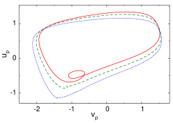
Figure 8: (Color Online). Evolution of attractor shape in the phase space. Theta-rhythm. Projection on the variables of the pyramidal cell. Minor loops, which correspond to subthreshold oscillations, shrink, turn into cusps and disappear.
Solid line: $G_{LP}$=0.09, dashed line: $G_{LP}$=0.2, dotted line: $G_{LP}$=0.4.

A similar process of deformation occurs on the other branch of solutions, which corresponds to the theta/gamma state. In this state, patches of full-scale spikes are separated by subthreshold oscillations (cf. Fig.4); the latter correspond to minor loops on the projections of respective phase portraits. In the course of increase of conductance $G_{LP}$, the shape of the attracting orbit is subjected to continuous deformation (similarly to that shown in Fig. 8 for theta-rhythm): the minor loop gradually gets smaller, shrinks into a cusp and disappears completely. This process leads to gradual decrease and elimination of one of the maxima in the temporal pattern of the oscillations.

As seen in Fig. 6, the branch of theta/gamma oscillations is isolated in the parameter space. A closer look shows that its birth at low values of $G_{LP}$ begins with a very short segment of mixed-mode oscillations; they are present close to $G_{LP}$=0.0362, but already at $G_{LP}$=0.0363 the characteristic shape of periodic theta/gamma oscillations is established. On the other end of the branch, at $G_{LP}$=2.274, the limit cycle which corresponds to the theta/gamma rhythmic pattern, disappears in the saddle-node bifurcation.

III.5 Attraction basins of coexisting states

In further numerical simulations we studied the sensitivity of the system response with respect to a variation of initial conditions. At low (below 0.036) values of conductance $G_{LP}$ the oscillatory state of the gamma-type was reached for all tested initial conditions. On the other end, at sufficiently large (above 2.28) values of $G_{LP}$ the system appears to possess the unique attractor as well: now this is the limit cycle which corresponds to the theta regime. In between, the system is bistable.

For a case study we take the value $G_{LP}=0.8$, well inside the range of this parameter where the distinct oscillations of the theta type coexist with the theta/gamma rhythmic pattern.

The system has been scanned on a grid of initial conditions for variables $v_{i}$ and $u_{i}$ from -2 to 2: these ranges correspond to the maximal span of gamma and theta/gamma oscillations for pyramidal cells. The initial size of the mesh has been taken as 0.01$\times$0.01, and has been refined whenever necessary in order to resolve the fine details. It turned out that the choice of eventual attractor depends mostly on initial values of membrane potential and membrane variable of the slow cells.

To illustrate graphically the shape of the boundary between the attraction basins in the 12-dimensional space of initial values, we choose two characteristic intersections of this boundary with coordinate planes. The first one (left panel of Fig.9) is the plane upon which all coordinates except $v_{p}$ (voltage variable of the pyramidal cell) and $u_{L_{1}}$ (gating variable of the left slow cell) are set to zero. The plot shows two distinct regions of theta oscillations separated by a strip which belongs to the basin of the theta/gamma state. Both borderlines display rather mild variations. Notably, the initial value of $u_{L_{1}}$ should be sufficiently large in order to excite the theta oscillation: initial strong contrast between the $OLM$-cells (recall that $u_{L_{2}}$=0 upon this plane) would facilitate the onset of the large phase difference between them, imminent for the theta state.

The second coordinate plane corresponds to the case when only the voltage variables of the $OLM$-cells are initially excited whereas the rest of the variables starts from zero values. In this projection (right panel of Fig.9), the shape of attraction basins is much more intricate, with characteristic cusps, islands and narrow bridges between them. Here, again, we see that proximity between the initial states of the slow cells results, as a rule, in the eventual onset of the theta/gamma rhythmic pattern.

Experimentally relevant is the location of the border between the basins in terms of the membrane voltage of slow cells. Numerics shows that this border (not presented graphically) looks quite simple: within the studied range of $v_{p}$ there exists a threshold value of voltage $v_{L_{1,2}}\approx 0.14$ below which the unit oscillates in the theta/gamma rhythm whereas above it the theta rhythm has been registered.

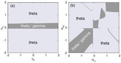
Figure 9: (Color Online). Projections of attraction basins of coexisting rhythmic patterns. $G_{BL_{1}}=0.06,G_{BL_{2}}=0.03$, $G_{LP}=0.8$. Dark grey: attraction basin of the theta/gamma rhythm. Light grey: attraction basin of theta-oscillations. (a): initial values for voltage of the pyramidal cell vs. membrane variable of the left slow cell; the rest of variables is set to zero. (b): initial values for membrane variables of two slow cells; the rest of variables is set to zero.

III.6 Variation of asymmetry between BL-synaptic connections

In order to elucidate the possible role of asymmetry in the pattern of synaptic connections, we performed calculations at different values of the ratio $G_{BL_{1}}/G_{BL_{2}}$. Decreasing this ratio from 2 to 1, we have detected qualitative distinction only at very low values of conductance $G_{LP}$; otherwise, the results were largely similar to the ones described in the previous subsections.

In the symmetric case $G_{BL_{1}}=G_{BL_{2}}$, the system possesses the invariant “diagonal” subspace in which the values of variables for the two slow cells coincide (hence, the phase shift between them is absent). Surprisingly, the states from this subspace are stable not only at moderate values of $G_{LP}$ which correspond to the attractor of the theta/gamma type, but at low values of this parameter as well, where the temporal pattern belongs to the gamma-type. In contrast to the previously described gamma-oscillations, in this state the phase shift between the slow cells is absent; they oscillate in unison. Below we call this regime a “symmetric gamma-state”. If the conductance $G_{LP}$ is set below $0.0016$, symmetric gamma-oscillations are chaotic. Above this value of $G_{LP}$ the periodic gamma-state is observed; in a narrow interval close to $G_{LP}$=0.036 its regular pattern is transformed (via the mixed-mode) into the periodic theta/gamma oscillation. Outside the diagonal subspace there exists another,“asymmetric” oscillatory state which has a shape of gamma-oscillations with a phase difference of $2\pi/3$ between the slow cells and is akin to the gamma-state described in the Sect. III.1.

Accordingly, at sufficiently low values of $G_{LP}$, two qualitatively different types of gamma-oscillations coexist: a symmetric one and an asymmetric one in which there is a phase lag between the slow cells. The asymmetric type, in its turn, consists of two different limit cycles: the state in which the phase of the cell $L_{1}$ is $2\pi/3$ ahead of $L_{2}$, as well as its mirror counterpart in which $L_{2}$ is “leading”.

Depending on the initial conditions, the symmetrical network can display either of these three gamma-patterns. Being structurally stable, all three limit cycles survive introduction of weak asymmetry between the connections; of course, the former symmetric state develops in this case a small phase shift between the slow cells. Increase of $G_{BL_{1}}$ at constant value of $G_{BL_{2}}$ initially results in the growth of the attraction basin of the oscillation with leading $L_{1}$ at the cost of the basins of two other gamma-states. Further growth of $G_{BL_{1}}$ brings about saddle-node bifurcations in which at first the former symmetric gamma-state and then the gamma-state with leading $L_{2}$ disappear.

For example, at $G_{BL_{2}}$=$G_{LP}$=0.03 all three gamma patterns coexist in the range of values of $G_{BL_{1}}$ between 0.03 and 0.03774. The saddle-node bifurcation of periodic orbits on the right border of this interval destroys the former symmetric pattern. Of the two remaining states with phase shift close to $2\pi/3$, the pattern with leading $L_{2}$ disappears in the saddle-node bifurcation at $G_{BL_{1}}$=0.04732: beyond this value of $G_{BL_{1}}$ only one pattern of the gamma-type can be observed.

Let us return to characterization of the symmetric network with $G_{BL_{1}}=G_{BL_{2}}$=0.03. Except for the “unison” symmetric gamma-state, the appearance and properties of the gamma- and theta-oscillations display only small quantitative difference from the case $G_{BL_{1}}\neq G_{BL_{2}}$ described in the preceding sections. Two paragraphs above we have characterized solutions which at low values of $G_{LP}$ look like a gamma-oscillation with a phase shift between the slow cells close to $2\pi/3$. At around $G_{LP}$=0.073 this pattern is rapidly transformed (via the mixed-mode oscillation) into the theta-rhythm in which the slow cells oscillate in the antiphase; stable theta-oscillations persist in the whole studied range $G_{LP}\leq 3$. Similarly to the asymmetric case, at sufficiently high values of conductance $G_{LP}$, theta/gamma-state has not been observed, and the theta-oscillations are the only attractor of the system (cf. Fig. 6). In absence of symmetry between $BL_{1,2}$, the periodic theta/gamma state is eliminated in the course of the saddle-node bifurcation. In the symmetric case, this bifurcation is replaced by the inverse pitchfork bifurcation; for $G_{BL_{1}}=G_{BL_{2}}$=0.03 this event takes place at $G_{LP}$=2.014. As a result, the periodic solution of the theta/gamma type persists at higher values of $G_{LP}$ as well, but is attracting only in the invariant “diagonal” subspace $u_{L_{1}}=u_{L_{2}}$ and $v_{L_{1}}=v_{L_{2}}$. A weak violation of the symmetry in initial conditions leads to creation and growth of the phase shift between the slow cells, which eventually destroys the theta/gamma oscillations and replaces them by the theta-rhythm.

Concerning the border between attraction basins in case of hysteresis between theta and theta/gamma rhythms, merely the quantitative shift due to variation of the ratio $G_{BL_{1}}/G_{BL_{2}}$ has been observed; the shape of the basins has been largely preserved. Compared to Fig. 9(a), in the symmetric case $G_{BL_{1}}=G_{BL_{2}}$ the attraction basin of the theta/gamma state is slightly broader. In contrast, projection of attraction basins for membrane variables of two slow cells (analog of Fig. 9(b), which is symmetric with respect to the diagonal) displays a slight narrowing of the theta/gamma region. Besides, we have observed that symmetry in the conductances $G_{BL_{1,2}}$ lowers the threshold values of the membrane potentials $v_{L_{1,2}}$, which are necessary for the onset of the theta rhythm.

IV Discussion

In the preceding sections we have presented a minimalistic model for a working unit of neuronal network in the hippocampus. Below we briefly discuss a few important aspects of this model.

IV.1 Minimality of network

Arguably, the size of the ensemble cannot be further reduced without introducing drastic distortions into collective dynamics. For example, omittance of one of the slow $L$ cells would disable the theta rhythm. As seen in Fig.5, in this regime two $L$ cells are oscillating in the antiphase, and the fast pyramidal cell exhibits two spikes within a complete oscillation cycle: one spike comes shortly before the maximum of $L_{1}$ and the other one precedes the maximum of $L_{2}$. As soon as one slow partner is removed, this rhythmic pattern becomes impossible.

Further, our numerical experiments show that if the basket cell is removed from the configuration, the rhythmic patterns persist but their dependence on the strength of the coupling between the remaining pyramidal cell and the slow cells is weakened. If the configuration of connections is symmetric, the system is restricted to only one scenario of the onset of rhythms which is mostly determined by the choice of initial conditions. This seems to contradict to the experimental evidence which confirms that switching between the regimes depends on the coupling strength Gloveli . In the attempts to counteract the removal of the basket cell by asymmetry in the connections from the pyramidal cell to OLM-cells we observed that the region of existence of the theta/gamma regime is significantly reduced.

Thus, we suppose that presence of the basket cell allows the neuronal network not only to “maneuver” between different scenarios of emergence of all rhythms but also to expand the region of existence of the theta/gamma regime.

The role of asymmetry in this context is twofold. On the one hand, as shown in Sect. III.6, the symmetric case possesses more attractors, which enhances the flexibility of the network. On the other hand, reduction of variability in the strongly asymmetric network means increase in the robustness, which can also be useful in certain situations.

IV.2 Possible implications for larger networks

We have started this section by defending our choice of the minimal model. Here we turn to the “inverse” question: are patterns, generated by this minimal unit, recognizable on the background of large hyppocampal networks? Numerous experiments in the hyppocampal areas CA1 and CA3 unambiguously confirm existence of all described oscillatory states: the gamma, the theta and the theta/gamma Bur ; Glov ; Gloveli . Furthermore, in-vitro technique of directional cross-sections in the hyppocampus has allowed to single out the patterns: in longitudinal sections mostly the theta rhythm is recovered, whereas oscillations of gamma and theta/gamma are typical for transverse and “medium” (so-called coronal) slices. This has to do with morphology of the participating cells. The OLM cells are arborized (possess dendritic structure) mostly in the longitudinal direction. In longitudinal slices synaptic connections from these cells to the pyramidal and basket ones are at the strongest; this results in the synchronous theta rhythm in the area CA3 Glov ; Gloveli ; Tor . In other directions arborization is much less pronounced; hence, the relative role of the OLM cells is weaker, and one observes mostly the gamma and theta/gamma oscillations produced by interaction of pyramidal and basket cells.

Other kinds of cells contribute to shaping and maintenance of rhythmic patterns as well: the study Klaus lists at least 21 classes of inhibitory interneurons which participate in the oscillations. Anyone of them could be a part of the minimal module. However, high synchrony between inhibitory interneurons responsible for gamma-rhythm Glov ; Haj allows to restrict modeling to just one type: we have chosen the basket cells, whose interactions with pyramidal cells are well investigated experimentally. On adding the OLM cells which are required for the generation of the theta state, we get by with just three types of cells in a module.

How do such “modules” interact with each other in a large-scale network? What cells mediate the interactions? Which type of connection – excitatory or inhibitory – should be considered? From the point of view of morphological properties, briefly sketched above, it seems plausible that modules communicate with each other through OLM cells. The pyramidal and basket cells have been shown to be involved mostly in locally synchronized gamma oscillations Glov . Within this conjecture, OLM cells of a module can inhibit pyramidal cells in the neighboring modules Tor . As for interactions between OLM and basket cells in large networks, reliable experimental data are still missing.

Spatial-temporal patterns in big networks depend on the strength of connection between modules. For the case of strong coupling there is experimental evidence of phase theta waves Lub . In contrast, moderate coupling leads to spatial-temporal gamma oscillations which modulate slow theta patterns (clusters) Bel . Notably, such patterns are sensitive to the phase shift between the OLM cells. Finally, if the interaction is sufficiently weak, the modules oscillate independently of each other. In this case, rhythms found in a single module, persist, and presence of neighbors results, mostly, in shifting the transitions between them.

IV.3 Multistability

Hysteretic properties, akin to the described effect of multistability, have been registered in experiments with subthalamic neurons Kass . In these experiments application of different bias currents and shifting of the baseline membrane potential resulted in the onset of such different regimes as tonic firing, rhythmic bursts or silent upstate. According to the experimentalists, multistability can be controlled by dynamics of ionic channels Kass .

In our model, depolarization of initial membrane potential of L-cells results in the onset of the theta/gamma regime, but stronger depolarization switches the latter to pure theta oscillations.

To our knowledge, multistability of the discussed kind has not yet been registered in CA3, either in experiments or in existing theories. (Metastable states in large sections of CA3, experimentally found in  Sasaki , refer to alternating activity of different groups of neurons, and not to different rhythmic patterns). In particular, the authors of the more detailed model described in Gloveli do not report on coexistence of attractors. Transitions between rhythms can be related to physiological state of a cell. The OLM cells are known to possess two specific ionic currents responsible for the onset of theta rhythm Gloveli ; Sar . One of these currents is activated by the strong hyperpolarization, whereas the latter, in turn, is switched on by depolarization. These states correspond, respectively, to the top and bottom stripes in the left panel of Fig. 9, therefore in the corresponding ranges of potentials theta regime is established. For the initial conditions from the “middle” stripe these currents are modest, hence theta rhythm cannot develop, and theta/gamma rhythm is observed instead. This interpretation requires, of course, an experimental testing.

References

- (1) A. T. Winfree, The Geometry of Biological Time, Springer, NY, 1980.
- (2) J. O’Keefe and M. L. Recce, Hippocampus 3, 317 (1993).
- (3) G. Buzsaki, Neuron 33, 325 (2002).
- (4) K. D. Harris, J. Csicsvari, H. Hirase, G. Dragoi and G. Buzsaki, Nature 424, 552 (2003).
- (5) N. Hajos, O. Paulsen, Neuronal Networks 22, 1113 (2009).
- (6) T. Gloveli, T. Dugladze, S. Saha, H. Monyer, U. Heinemann, R. D. Traub, M. A. Whittington, E.H. Buhl, J. Physiol. 562.1, 131 (2005).
- (7) T. Gloveli, T. Dugladze, H. G. Rotstein, R. D. Traub, H. Monyer, U. Heinemann, M. A. Whittington, N. J. Kopell, PNAS 102, 13295 (2005).
- (8) G. Maccaferri, G. J. McBain, J. Physiol. 497.1, 119 (1996).
- (9) E. O. Mann, C. A. Radcliffe, O. Paulsen, J. Physiol. 562.1, 55 (2005).
- (10) T. Klausberger, P. Somogyi, Science 321, 53 (2008).
- (11) F. Froehlich, T. J. Sejnowski, M. Bazhenov, J. Neuroscience 30, 10734 (2010).
- (12) D. Durstewitz, Neuronal Networks 22, 1189 (2009).
- (13) J. I. Kass, I. M. Mintz, PNAS 103, 183 (2006).
- (14) T. Sasaki, N. Matsuki, Y. Ikegaya, J. Neuroscience 27, 517 (2007).
- (15) P. Hahn and D. M. Durand, J. Comp. Neuroscience 11, 5 (2001).
- (16) P. Andersen, The Hippocampus book, Oxford University Press (2007).
- (17) N. Kopell, C. Borgers, D. Pervouchine, P. Malerba, A. Tort, In: Hippocampal Microcircuits: A Computational Modeller’s Resource Book., Chapter 15, Eds. V. Cutsuridis, B.P. Graham, S. Cobb, I. Vida. Springer 2010.
- (18) P. J. Siekmeier, Behav. Brain Res. 200, 220 (2009).
- (19) F. Fröhlich and M. Bazhenov, Phys. Rev. E 74, 031922 (2006).
- (20) M. Rabinovich, R. Huerta, M. Bazhenov, A. K. Kozlov, H. D. I. Abarbanel, Phys. Rev. E 58, 6418 (1998).
- (21) R. D. Traub, A. Bibbig, F. E. N. LeBeau, E. H. Buhl, M. A. Whittington, Ann. Rev. Neuroscience 27, 247 (2004).
- (22) B. H. Singer, M. Derchansky, P. L. Carlen, and M. Zochowski, Phys. Rev. E 73, 021910 (2006).
- (23) H. D. I. Abarbanel, S. S. Talathi, L. Gibb, M. I. Rabinovich, Phys. Rev. E 72, 031914 (2005).
- (24) M. A. Zaks, X. Sailer, L. Schimansky-Geier, A. Neiman, Chaos 15, 026117 (2005).
- (25) D Hennig, L. Schimansky-Geier, Physica A 387, 967 (2008).
- (26) R. FitzHugh, Mathematical models of excitation and propagation in nerve, in Biological Engineering, edited by H.P. Schwan (McGraw-Hill Book Co., N.Y. 1969), Chap. 1, p. 1.
- (27) M. J. Gilles, R. D. Traub, F. N. LeBeau, C. H. Davies, T. Gloveli, E. H. Buhl, M. A. Whittington, J. of Physiol. 543.3, 779 (2002).
- (28) M. Brons, T. J. Kaper, H. G. Rotstein (Editors). Mixed Mode Oscillations: Experiment, Computation, and Analysis, Focus Issue of Chaos 18 (2008).
- (29) F. Saraga, C. P. Wu, L. Zhang, F. K. Skinner, J. Physiol. 552.3, 673 (2003).
- (30) A. Tort, H. G. Rotstein, T. Dugladze, T. Gloveli, PNAS 104, 13490 (2007).
- (31) E. V. Lubenov, A. S. Siapas, Nature 459, 534 (2009).
- (32) M. A. Belluscio, K. Mizuseki, R. Schmidt, R. Kempter, G. Buzsaki, J. Neuroscience 32, 423 (2012).