Gibbs free energy and Helmholtz free energy
for a three-dimensional Ising-like model

Abstract

The critical behavior of a $3D$ Ising-like system is studied at the microscopic level of consideration. The free energy of ordering is calculated analytically as an explicit function of temperature, an external field and the initial parameters of the model. Within a unified approach, both Gibbs and Helmholtz free energies are obtained and the dependencies of them on the external field and the order parameter, respectively, are presented graphically. The regions of stability, metastability, and unstability are established on the order parameter–temperature plane. The way of implementation of the well-known Maxwell construction is proposed at microscopic level. Ising-like model, critical behavior, external field 05.50.+q, 05.70.Ce, 64.60.F-, 75.10.Hk

Abstract

В данiй роботi на мiкроскопiчному рiвнi розгляду вивчається критична поведiнка тривимiрної iзiнгоподiбної системи. Аналiтично обчислюється вiльна енергiя впорядкування як функцiя температури, зовнiшнього поля i початкових параметрiв моделi. В межах запропонованого пiдходу отримано вирази для вiльної енергiї Гiббса i Гельмгольца, їх залежностi вiд поля i параметра порядку приведенi також графiчно. На площинi параметр порядку–температура знайденi областi стабiльностi, метастабiльностi та нестабiльностi. Запропоновано спосiб реалiзацiї правила Максвелла на мiкроскопiчному рiвнi. модель Iзiнга, критична поведiнка, зовнiшнє поле

1 Introduction

Basic principles of phenomenological theory for second order phase transitions (PT) were formulated by Landau in late 30–40s [1, 2], originally to describe superconductivity. The key assumption of the theory is that in the vicinity of the critical point, the free energy can be expanded in a power series in the order parameter, the equilibrium value of which is found to obey the minimum condition for free energy. As is now known [3], this expansion is well defined in the neighborhood of $T_{\mathrm{c}}$ (critical value of temperature) except for a narrow interval determined by the Ginzburg criterion [4]. In this interval, the crucial role is played by the order parameter fluctuations while Landau’s theory is essentially a mean-field theory. Nevertheless, it is of great use as a qualitative tool for understanding the nature of PT.

The above mentioned power series expansion is often called Landau’s free energy. It turns out that similar quantity can also be derived (not constructed) in a theory considering PT at a microscopic level. Indeed, in the collective variables (CV) method proposed in [5, 6] to describe the critical behavior of spin systems, such a quantity appears in a natural way. In particular, a microscopic analogue of Landau free energy was calculated in [7], where the Ising-like system was considered in zero external field.

The purpose of the present paper is to extend the results obtained earlier by the CV method for physical characteristics of 3D Ising-like model to the presence of an external field and look at what is going on when the field changes sign. As a result, we obtain the Gibbs free energy, Helmholtz free energy, and the order parameter and establish the regions of stability, metastability, and unstability for the system under investigation.

2 Method

In our research we consider the system of $N$ Ising spins placed on sites of a simple cubic lattice of the spacing $c$. The Hamiltonian of such a system in an external field is well known

$$H=-\frac{1}{2}\sum_{{i},{j}}\Phi(r_{{i},{j}})\sigma_{{i}}\sigma_{{j}}-{\cal{H}}\sum_{{i}}\sigma_{{i}}\,.$$ (1)

Here, $\Phi(r_{{i},{j}})$ is a short-range interaction potential between spins located at the $i$-th and $j$-th sites, the spin variables $\sigma_{{i}}$ take on values $\pm 1,$ ${\cal H}$ is the external field. We do not restrict the summation in (1) to the nearest neighbors. To this end, $\Phi(r)=\text{const}\times\exp{(-r/b)}$ can be chosen as the interaction potential with an effective range $b$.

It is also known that this problem has not yet been solved. Universal critical characteristics of three-dimensional (3D) systems are successfully described in a variety of approaches. Among them it is worth mentioning the field theoretical and renormalization group (RG) methods [8], which also enable one to calculate nonuniversal characteristics (critical amplitudes, critical temperatures), but without taking into account the dependency on initial parameters of the Hamiltonian. An alternative method for theoretical investigation of the model under consideration is the method of CV [5], which has an advantage of being a successive microscopic approach, which, in turn, makes it possible for thermodynamic functions and physical characteristics of the system to be explicitly obtained as functions of temperature, the field, and microscopic parameters of the model.

In the framework of the ‘‘$\rho^{4}$-model’’ approximation the functional representation for the partition function in terms of CV $\rho_{\textbf{k}}$ is as follows:

$$Z = Z_{0}\int(d\rho)^{N_{0}}\exp\bigg{[}a_{1}\sqrt{N_{0}}\rho_{0}-\frac{1}{2}\sum_{\textbf{k}\in{\cal{B}}_{0}}d(k)\rho_{\textbf{k}}\rho_{-\textbf{k}}-$$ (2)

$$- \frac{a_{4}}{4!}N_{0}^{-1}\sum_{\textbf{k}_{i}\in{\cal{B}}_{0}}\rho_{\textbf{k}_{1}}\ldots\rho_{\textbf{k}_{4}}\delta_{\textbf{k}_{1}+\ldots+\textbf{k}_{4}}\bigg{]}.$$

Here, the quantity $d(k)$ contains the Fourier transform of the interaction potential

$$d(k)=a_{2}+\beta\Phi(0)\bar{\Phi}-\beta\Phi(k).$$ (3)

The explicit expressions for $a_{n}$ can be found in [9] (equation (1.25)) , $N_{0}=N/s_{0}^{3}$ where the quantity $s_{0}$ defines the region of validity for the parabolic approximation of Fourier transform of the interaction potential (for details, see [10]). The summation in (2) is performed over wave vectors of the first Brillouin zone corresponding to a reciprocal effective lattice with the lattice constant $cs_{0}$.

In the work [11] the method for calculation of the partition function (2) of the model near the second order PT point was generalized to the case of the presence of the fixed external field of an arbitrary magnitude. Unlike the work [12], here no assumption concerning either the strength or the weakness of the applied field is made and, therefore,no perturbation series are used. The calculation procedure is based on Kadanoff’s idea of constructing effective spin blocks [13]. We divide the phase space of the CV $\rho_{\textbf{k}}$ into layers, the RG parameter being $s$, and average the Fourier transform of the potential in each $n$-th layer. The first step in calculating equation (2) is to integrate over $\rho_{\textbf{k}}$ with $k\in[k_{\mathrm{max}},k_{\mathrm{max}}/s],$ $k_{\mathrm{max}}={\pi}/{cs_{0}}.$ The result of integration proves to be represented in the form of the initial expression, equation (2), with renormalized coefficients $a_{1}^{(1)},$ $d_{1}(k),$ and $a_{4}^{(1)}.$ If we perform a step-by-step integration of the partition function over $n_{p}$ layers, we arrive at

$$Z=Z_{0}\big{[}Q(d)\big{]}^{N_{0}}\bigg{(}\prod_{n=1}^{n_{p}}Q_{n}\bigg{)}Z_{\rm LGR}\,.$$ (4)

The partial partition functions $Q_{n}$ of the $n$-th level are characterized by a set of coefficients $a_{1}^{(n)},$ $d_{n}(0)$, $a_{4}^{(n)}$, for which the recurrence relations (RR) hold (the work [9] is devoted to this problem). The quantity $n_{p}$ is called the exit point from the critical regime of the order parameter fluctuations. It defines the number of iterations at which the system is still in the scaling region.

In [12], two regions in $(h,\tau)$-plane were distinguished, which are of weak and of strong field. The calculations in the regions were performed using different forms of exit points. These quantities were subject to certain conditions which we do not discuss in the present work. If the field was considered to be strong, the formula $n_{p}=n_{h}=-\ln{\tilde{h}}/\ln{E_{1}}-1$ was used, while in the case of a weak field another expression $n_{p}=m_{\tau}=-\ln{\tilde{\tau}}/\ln{E_{2}}-1$ was taken. Hence, the question immediately arises what should be done at intermediate values of a field. The problem is solved by constructing a new expression for the exit point, proposed in [11]:

$$n_{p}=-\frac{\ln{\left(\tilde{h}^{2}+{h_{\mathrm{c}}^{(\pm)}}^{2}\right)}}{2\ln{E_{1}}}-1,$$ (5)

where some temperature fields $h_{\mathrm{c}}^{(+)}=|\tau|^{p_{0}}$ and $h_{\mathrm{c}}^{(-)}=|\tau_{1}|^{p_{0}}$ are introduced, $p_{0}=\ln{E_{1}}/\ln{E_{2}}$ is the so-called ‘‘gap exponent’’ [14], the signs ‘‘+’’ and ‘‘–’’ are related to $T>T_{\mathrm{c}}$ and $T<T_{\mathrm{c}}$ respectively, and

$$\tilde{h}=\frac{s_{0}^{3/2}}{h_{0}}h,\quad h=\beta{\cal{H}},\quad\quad\quad\tilde{\tau}=\frac{c_{k_{1}}}{f_{0}}\tau,\quad\tau_{1}=-E_{2}^{n_{0}}\tau,\quad\tau=\frac{T-T_{\mathrm{c}}}{T_{\mathrm{c}}}\,.$$ (6)

The quantities $E_{1}$ and $E_{2}$ are the eigenvalues of the matrix of the RG transformation linearized near the fixed point of RR.

In the limiting cases, as $h\rightarrow 0$ or as $\tau\rightarrow 0,$ equation (5) takes on the form of $m_{\tau}$ or $n_{h},$ respectively, and therefore can be applied to the case of an arbitrary field. Nevertheless, it is worth mentioning that the inequality $\tilde{h}\gg h_{\mathrm{c}}$ defines a strong field, and $\tilde{h}\ll h_{\mathrm{c}}$ defines a weak field. Note also that there is an arbitrariness in choosing $n_{p},$ which is discussed in [11, 10] in more detail. What is important is that for $n>n_{p}$ one should be able to integrate the partition function with Gaussian measure density.

Table 1: Numerical values of the parameters used in present calculations.

$b/c$	$\beta_{\mathrm{c}}\Phi(0)$	$s_{0}$	$f_{0}$	$h_{0}$	$c_{k_{1}}$	$\phi_{0}$	$\Phi_{f}$	$n_{0}$
0.3	1.6411	2.0	0.5	0.760	1.1762	0.5938	0.105	0.5

We will adhere to the approach adopted in [15], where the coefficients $c_{k_{1}},$ $f_{0},$ $h_{0}$ are also defined (see equations (4.4), (4.17), (4.23), and (4.49) in [15]), and take $E_{1}=24.551,$ $E_{2}=8.308.$ The information on the physical meaning of coefficient $n_{0}$ can be found in [16]. Numerical values of all coefficients used to obtain the final graphical results are presented in table 1. It is worth stressing that having fixed the value of RG parameter $s=s^{*}$ ($s^{*}=3.5977$ in the present calculation), there remains only one initial parameter, which is the ratio of the effective range of interaction $b$ to the lattice constant $c$. All the other coefficients can be expressed via $b/c$ [10, 17].

3 Results and discussion

Based on the above mentioned method, in the work [11] as well as in [16] free energy of 3D Ising-like model was calculated as a logarithm of the partition function (4) multiplied by $-kT$ and presented in the form of several contributions

$$F(\tau,h)=F_{a}+F_{s}^{(\pm)}+F_{0}^{(\pm)}.$$ (7)

Here, the term $F_{a}$ is the analytical part of free energy and does not affect the critical behavior of the system. The last two terms in r.h.s. of (7) have non-analytical dependence on temperature and on the external field. The explicit expressions for $F_{s}^{(\pm)}$ and $F_{0}^{(\pm)}$ are

$$F_{s}^{(\pm)}(\tau,h)=-kTN\gamma_{s}^{(\pm)}\left(\tilde{h}^{2}+{h^{(\pm)}_{\mathrm{c}}}^{2}\right)^{\frac{d}{d+2}},$$ (8)

and

$$F_{0}^{(\pm)}(\tau,h)=-kTNE_{0}(\sigma_{\pm}).$$ (9)

The quantity $\gamma_{s}^{(\pm)}$ from (8) includes contributions from the critical regime of the order parameter fluctuations and from the limiting Gaussian regime (LGR)(for details, see [11, 16]). The mentioned critical regime is characterized by the RG symmetry.

The quantity $E_{0}(\sigma_{\pm})$ is the contribution from the collective variable $\rho_{0}$. As is known from the theory of CV [5], the mean value of $\rho_{\textbf{k}=0}$ is connected with the order parameter and consequently the quantity $F_{0}$ is the free energy of ordering [7]. If there is no external field, $F_{0}$ is analogous to Landau’s free energy in phenomenological theory of second order PT [7]. Since we work in the ensemble of $N$ particles, with field $h$ and temperature $\tau$ being independent variables, this analogy is now not direct. Following Stanley [14], and based on convincing arguments of the work [18], we associate the partition function of our model with Gibbs free energy. An appropriate thermodynamic potential is Gibbs free energy provided the magnetic field and temperature are independent (‘‘natural’’) variables. If the role of independent variables is played by an order parameter (here magnetization per spin) and temperature, then the thermodynamic potential associated with the partition function is Helmholtz free energy. Hence, Landau’s free energy is rather Helmholtz than Gibbs one. The expressions (7)–(9) in turn present Gibbs free energy for the considered model, although this was not specified in earlier works, particularly in [11, 16]. Therefore, in order to obtain a microscopic analogue of Landau’s energy one should perform the Legendre transformation. Let $A_{0}$ denote this analogue. Then,

$$A_{0}(\tau,M)=F_{0}+M_{0}{\cal{H}},$$ (10)

where $M_{0}$ is the magnetization of the system under consideration such that

$$M_{0}=-\frac{1}{N}\frac{\partial{F_{0}}}{\partial{\cal{H}}}=\frac{\partial{E_{0}}}{\partial{h}}\,.$$ (11)

The expression for $E_{0}(\sigma_{\pm})$, which was found in [11] (see equation (4.4) there) for $T>T_{\mathrm{c}}$ and in [16] (see equation (4.3) there) for $T<T_{\mathrm{c}},$ reads

$$E_{0}(\sigma_{\pm})=h\sigma_{\pm}-\frac{1}{2}d_{n_{p}+2}(0)\sigma_{\pm}^{2}-\frac{s_{0}^{3}s^{3(n_{p}+2)}}{4!}a_{4}^{(n_{p}+2)}\sigma_{\pm}^{4}\,.$$ (12)

The quantity $\sigma_{\pm}$ was found from condition

$$\frac{\partial{E_{0}(\sigma_{\pm})}}{\partial{\sigma_{\pm}}}=0$$ (13)

in the form

$$\sigma_{\pm}=\sigma^{(\pm)}_{0}s^{-(n_{p}+2)/2}.$$ (14)

This results in the cubic equation for $\sigma^{(\pm)}_{0}$

$$\sigma_{0}^{3}+p\sigma_{0}+q=0$$ (15)

with coefficients

$$p = 6s_{0}^{-3}r_{n_{p}+2}/u_{n_{p}+2}\,,$$

$$q = -6s_{0}^{-9/2}s^{5/2}\frac{h_{0}}{u_{n_{p}+2}}\frac{\tilde{h}}{\left(\tilde{h}^{2}+{h^{(\pm)}_{\mathrm{c}}}^{2}\right)^{1/2}},$$ (16)

where the denotations $r_{n}$ and $u_{n}$ are connected with $d_{n}(0)$ and $a_{4}^{(n)}$ through $d_{n}(0)=s^{-2}r_{n}$, $a_{4}^{(n)}=s^{-4}u_{n},$ and according to [11, 16] are expressed as

$$r_{n_{p}+2} = \beta_{\mathrm{c}}\Phi(0)f_{0}\left(-1\pm\tilde{\tau}E_{2}^{n_{p}+2}\right),$$

$$u_{n_{p}+2} = [\beta_{\mathrm{c}}\Phi(0)]^{2}\phi_{0}\left(1\pm\tilde{\tau}E_{2}^{n_{p}+2}\Phi_{f}\right).$$ (17)

Note, that the coefficients $p$, $q$ should be marked by the superscript $\pm$ (as should be done for $n_{p}$ from (5)), but where it does not cause confusion, we drop this superscript out. One should just remember about a difference in temperature scales between the cases of $T>T_{\mathrm{c}}$ and of $T<T_{\mathrm{c}}.$

Equation (15) can be solved by Cardano’s method. The solutions are presented graphically in figure 1. From the plot we see that for a given value of field there exists some temperature $\tau_{0}<0$ such that equation (15) has three real solutions for $\tau\leqslant\tau_{0}$ and one real solution for $\tau>\tau_{0}.$ This quantity, $\tau_{0},$ corresponds to the condition $Q=0$ where $Q$ is the discriminant of the cubic equation (15):

$$Q=(p/3)^{3}+(q/2)^{2}$$ (18)

with $q$ and $p$ from (3). When $h=0$, then $\tau_{0}=0.$ If $h\neq 0,$ then $\tau_{0}$ is determined by setting r.h.s. of (18) equal to zero. In [16], $\tau_{0}$ was found numerically and the plot of $\tau_{0}$ versus $h$ was drawn. As we will see in what follows, the solution $\tau_{0}=\tau_{0}(h)$ to the equation $Q=0$ defines a curve in ‘‘order parameter–temperature’’ plane which can be identified with the spinodal of a fluid.

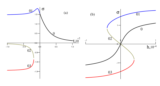
Figure 1: (Color online) Solutions of cubic equation (15) (a) as functions of temperature for $h=10^{-4}$; (b) as functions of field for $\tau=\pm 10^{-3}.$ The curves marked by ‘‘0’’ correspond to the real solutions at $\tau\geqslant 0;$ marked by ‘‘01’’, ‘‘02’’, and ‘‘03’’ denote different solution at $\tau<0.$ In this respect, we will refer to the solutions as $\sigma_{0}^{(+)}$ and $\sigma_{0i}^{(-)}$ ($i=1,2,3$).

Taking into account (5), and (14), the quantity $E_{0}(\sigma)$ takes on

$$E_{0}(\sigma)=he_{0}^{(\pm)}\left(\tilde{h}^{2}+{h_{\mathrm{c}}^{(\pm)}}^{2}\right)^{\frac{1}{2(d+2)}}-e_{2}^{(\pm)}\left(\tilde{h}^{2}+{h^{(\pm)}_{\mathrm{c}}}^{2}\right)^{\frac{d}{d+2}},$$ (19)

where we have introduced the following notation

$$e_{0}^{(\pm)} = \sigma_{0}^{(\pm)}s^{-1/2},$$

$$e_{2}^{(\pm)} = \frac{1}{2}{\sigma_{0}^{(\pm)}}^{2}s^{-3}\left(r_{n_{p}+2}+\frac{1}{12}u_{n_{p}+2}s_{0}^{3}{\sigma_{0}^{(\pm)}}^{2}\right).$$ (20)

In the previous works [11, 16, 10, 15] the system was considered in the external field $h\geqslant 0$. Analytical results for (Gibbs) free energy [11, 16], the order parameter [16, 10], and the susceptibility [10] were obtained. The purpose of this paper is to extend the method to the region $h<0$ and to take into account all solutions to the equation (15). We look at Gibbs free energy $F_{0}$ and at the contribution from it to the order parameter $M_{0}$ of equation (11). Thereupon, Helmholtz free energy is calculated.

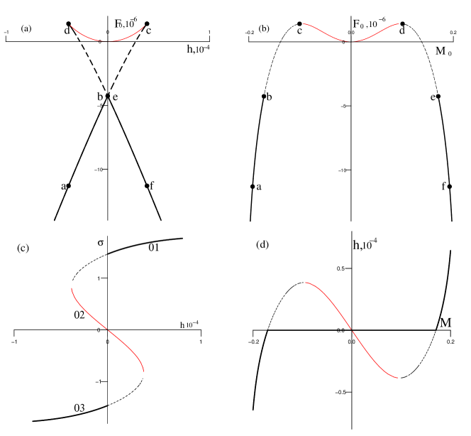
Figure 2: (Color online) A set of 4 pictures is placed for the sake of clarity. All are drawn for $\tau=-0.001.$ The top left is the field dependence of Gibbs free energy $F_{0}$. The top right shows $F_{0}$ against $M_{0}.$ The bottom left presents the solutions of the cubic equation (15). The bottom right is the equation of state for the system under consideration. The values of energies are normalized by dividing by $kTN.$ The points $a$ to $f$ represent some particular states of the system in different coordinates. See the text for details.

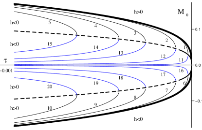
Figure 3: (Color online) The plot shows temperature dependence of magnetization calculated at different solutions to equation (15). Thick line is magnetization in zero external field and corresponds to the coexistence curve (binodal). In negative external field, the solution $\sigma_{01}$ gives rise to Curves 1–5 on the magnetization-temperature plane. In positive external field, $\sigma_{03}$ gives rise to Curves 6–10. Curves 11–20, which correspond to $\sigma_{02},$ can be interpreted as non-physical. Thick dashed curve corresponds to the saturation curve (spinodal). In order to recover that, one should compute magnetization corresponding to $\sigma_{01}$ at $h<0$ and $\tau_{0}=\tau_{0}(|h|)$ (upper branch) and corresponding to $\sigma_{03}$ at $h>0$ and $\tau_{0}=\tau_{0}(h)$ (lower branch). The magnitudes of field, at which the results are drawn, are $|h|=0,10^{-7},10^{-6},5\cdot 10^{-6},10^{-5},2\cdot 10^{-5}.$

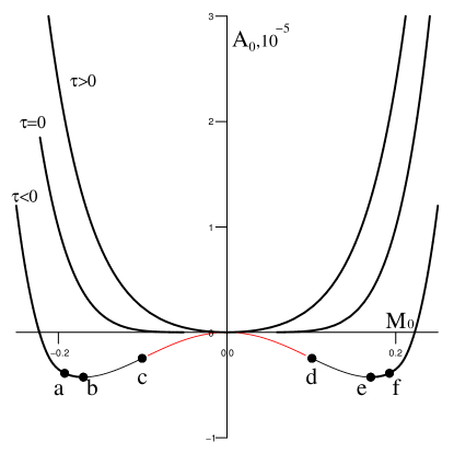
Figure 4: (Color online) Helmholtz free energy $A_{0}$ as a function of order parameter for three different temperatures $T<T_{\mathrm{c}}$ ($\tau=-0.001$), $T=T_{\mathrm{c}}$ ($\tau=0$), and $T>T_{\mathrm{c}}$ ($\tau=0.001$). The value is normalized by dividing by $kTN$.

The main results of this paper are presented in figures 2, 3, and 4. In figure 2 we can see: (a) Gibbs free energy $F_{0}$ as a function of the external field in low temperature region ($\tau=-0.001$); (b) a plot of $F_{0}$ versus $M_{0}$. Each of the points $a$, $b$, $c,\ldots$ represents a certain specific state of the system in different coordinates. Especially, points $a$, $c$, $d,$ and $f$ correspond to such a relation between the field $h$ and temperature $\tau$ that the equality $\tau=\tau_{0}(h)$ holds. Thus, in each of these we have $Q=0.$ Points $b$ and $e$ are associated with first order phase transition and correspond to $h=0$ and $\tau=-0.001.$ The isotherm in figure 2 (b) was drawn with the help of parametric representation {$F_{0}=F_{0}(h)$, $M_{0}=M_{0}(h)$}.

Recall that Gibbs free energy is a concave function of field [14]. Therefore, from figure 2 (a) we can conclude that the solution $\sigma_{02}^{(-)}$ gives rise to a non-physical result. It corresponds to the region of unstability ($c-d$ part of the curve in figure 2 (a), (b)). This is not surprising if we note that $\sigma_{02}^{(-)}$ maximizes $F_{0}.$ Solutions $\sigma_{01}^{(-)}$ at $h<0$ and $\sigma_{03}^{(-)}$ at $h>0$ correspond to the region of metastable states ($d-e$ and $b-c$ parts of the curve respectively). In the case of liquid-gas PT it would be the region between the binodal and the spinodal curves. Hence, we regard these results important from the perspective of using this method for description of the critical behavior in simple fluids.

Figure 2 (c) to some extent repeats figure 1 (b) and is placed here for convenience of representation. The quantity $\sigma_{0}$ is related to the scaling function of magnetization via formula (4.8) in work [16]. Finally, in figure 2 (d) the equation of state computed by means of (11) is presented at $\tau=-0.001.$

A more detailed representation of the equation of state is shown in figure 3. The derivatives of Gibbs free energy with respect to field are presented as functions of temperature, different solutions to equation (15) being taken into account. As we can see, such an accounting allows us to establish spinodal and binodal curves of the model and, in this respect, to find the stable, metastable, and unstable regions on ‘‘order parameter–temperature’’ plane.

The order parameter dependence of free energy $A_{0}$ is presented in figure 4 for three different temperatures $T>T_{\mathrm{c}}$, $T=T_{\mathrm{c}}$ and $T<T_{\mathrm{c}}$. Here again $a$, $b$, $c,\ldots$ denote the states as in figure 2. We can see that Helmholtz free energy has two minima below $T_{\mathrm{c}}.$ The equilibrium values for the order parameter are defined by these minima. Knowing their positions at different temperatures, we can recover the coexistence curve. Points $b$ and $e$ coincide with the minima at $\tau=-0.001.$ Note that based on the principle of minimum Gibbs free energy and from figure 2 (a), we can conclude that with the field changing from $h<0$ to $h>0$ the system will tend to move along $a-b-e-f$ part of the curve. Applied to Helmholtz free energy, it means that the system will tend to jump from state $b$ to state $e.$ Therefore, one may supplement figure 4 with a double-tangent construction. As a consequence, on $M_{0}-h$ plane we have a horizontal segment for $M_{0}$ at $h=0$ (see figure 2 (d)), which corresponds to a Maxwell construction derived at microscopic level. On the other hand, based on the maxima of Gibbs free energy with respect to $M_{0}$ (see figure 2 (b)), we are able to construct a saturation curve. Let us just remember that dependence $F_{0}$ on the order parameter is formal due to $M_{0}$ being not ‘‘natural’’ variable for $F_{0}.$ However, the same results for the binodal and the spinodal can immediately be obtained if one appropriately chooses the solutions to (15).

The forms of isotherms in figure 4 are similar to those in Landau’s theory [3]. However, the peculiar feature is that in the present work the free energy is an explicit function of temperature, external field and microscopic parameters (in the present case a ratio $b/c$) of the model, with a non-analytical dependence on its arguments. This gives rise to a non-classical critical behavior of the system, i.e., to the critical exponents taking on non-classical values. These values for the most important exponents are reported in table 2. There are also collected the values obtainable by CV method in higher, $\rho^{6}$ approximation as reported in Conclusions of the work [7]. Note that in our calculation we have neglected the critical exponent $\eta$ responsible for the behavior of the pair correlation function at $T=T_{\mathrm{c}}.$ Accounting for corrections to scaling is beyond the scope of the present paper as well. In table 2 the classic values for the critical exponents are presented as well as the results of other authors. We stick to the following notation. The temperature behavior of magnetization is governed by $\beta,$ of the heat capacity by $\alpha,$ of susceptibility by $\gamma,$ of the correlation length by $\nu.$ The field behavior of magnetization is governed by $\delta$, $M\sim|h|^{1/\delta}.$ We have calculated some of the exponents with the help of scaling laws. Based on earlier results [15], we are also able to estimate the critical exponents $\varphi$ and $\psi$ that describe the field behavior of the heat capacity, $C\sim|h|^{-\varphi},$ and of the entropy, $S\sim|h|^{\psi},$ respectively. Their numerical values are $\varphi=0.122$ and $\psi=0.539,$ which differ from $\varphi=0$ and $\psi=2/3$ in mean-field theory [14].

Table 2: Numerical values of the critical exponents. CV, collective variables method; MF, mean-field values; HT, high-temperature expansion results; FT, field theory approach.

	CV,	CV,	MF	HT [20, 19]	FT [21]
	$\rho^{4}$-model	$\rho^{6}$-model [7]
$\alpha$	0.185	0.088	0	0.110(1)0	0.109(4)00
$\beta$	0.302	0.319	1/2	0.3263(4)	0.3258(14)
$\gamma$	1.210	1.275	1	1.2373(2)	1.2396(13)
$\nu$	0.605	0.637	1/2	0.6301(2)	0.6304(13)
$\delta$	5	5	3	4.792	4.805

It should also be mentioned that the scaling properties for physical characteristics of the considered model are discussed in earlier works. In section 3 of the work [10] the scaling functions for (Gibbs) free energy, for the order parameter, and for susceptibility were calculated.

4 Conclusions

In this work, an analytical expression for Gibbs free energy of Ising-like system is obtained and investigated near the second order phase transition. The emphasis is made on the presence of the external field and on the situation where the field changes its direction. Some well-defined concepts of phenomenological theory of phase transitions - e.g. Landau’s energy, the Maxwell construction, the double-tangent construction - are derived and reexamined at microscopic level. We hope that the approach described and the results presented should be useful in further investigations of critical behavior in 3D Ising-like systems with analytical methods; in particular, in order to obtain the coexistence curve and the spinodal curve for a system at least in the vicinity of critical point. There exists a general belief [14, 20, 22] that simple fluids belong to the Ising universality class. Hence, we regard these results important from the perspective of using this method for description of the critical behavior in simple fluids.

Вiльна енергiя Гiббса та вiльна енергiя Гельмгольца для тривимiрної iзiнгоподiбної моделi

М.П. Козловський, Р.В. Романiк Iнститут фiзики конденсованих систем НАН України, вул. I. Свєнцiцького, 1, 79011 Львiв, Україна

References

- [1] Landau L.D., J. Exp. Theor. Phys., 1937, 7, 19 [Phys. Z. Sowjetunion, 1937, 11, 26].
- [2] Landau L.D., J. Exp. Theor. Phys., 1937, 7, 627 [Phys. Z. Sowjetunion, 1937, 11, 545].
- [3] Landau L.D., Lifshitz E.M., Statistical Physics (3rd ed., series Theoretical Physics, Vol. 5). Nauka, Moscow, 1976.
- [4] Ginzburg V.L., Fizika Tverdogo Tela, 1961, 2, 2031 [Sov. Phys. Solid State, 1961, 2, 1824].
- [5] Yukhnovskii I.R., Phase Transitions of Second Order: Collective Variables Method. World Scientific, Singapore, 1987.
- [6] Yukhnovskii I.R., Riv. Nuovo Cimento, 1989, 12, 1; doi:10.1007/BF02740597.
-
[7]
Yukhnovskii I.R., Kozlovskii M.P., Pylyuk I.V., Phys. Rev.
B, 2002, 66, 134410;
doi:10.1103/PhysRevB.66.134410. - [8] Zinn-Justin J., Phase Transitions and Renormalization Group. Oxford University Press, 2007.
- [9] Kozlovskii M.P., Condens. Matter Phys., 2005, 8, 473.
- [10] Kozlovskii M.P., Romanik R.V., Condens. Matter Phys., 2010, 13, 43004; doi:10.5488/CMP.13.43004.
- [11] Kozlovskii M.P., Condens. Matter Phys., 2009, 12, 151; doi:10.5488/CMP.12.2.151.
-
[12]
Kozlovskii M.P., Pylyuk I.V., Prytula O.O.,
Phys. Rev. B, 2006, 73, 174406;
doi:10.1103/PhysRevB.73.174406. - [13] Kadanoff L.P., Physics, 1966, 2, 263.
- [14] Stanley H.E., Introduction to Phase Transition and Critical Phenomena. Clarendon press, Oxford, 1971.
- [15] Kozlovskii M.P., Ukr. J. Phys., 2009, 5, 61 [in Ukrainian].
- [16] Kozlovskii M.P., Romanik R.V., J. Phys. Stud., 2009, 13, 4007.
- [17] Yukhnovskii I.R., Kozlovskii M.P., Pylyuk I.V., Microscopic Theory of Phase Transitions in the Three-dimentional Systems. Eurosvit, Lviv, 2001.
- [18] Castelano G., J. Magn. Magn. Mater., 2003, 260, 146; doi:10.1016/S0304-8853(02)01286-6.
- [19] Butera P., Comi M., Phys. Rev. B, 2005, 72, 014442; doi:10.1103/PhysRevB.72.014442.
- [20] Butera P., Pernici M., Phys. Rev. B, 2011, 83, 054433; doi:10.1103/PhysRevB.83.054433.
- [21] Zinn-Justin J., Phys. Rep., 2001, 344, 159; doi:10.1016/S0370-1573(00)00126-5.
- [22] Fisher M.E., Zinn S.-Y., Upton P.J., Phys. Rev. B, 1999, 59, 14533; doi:10.1103/PhysRevB.59.14533.