Anisotropic Universe Models in Brans-Dicke Theory

Abstract

This paper is devoted to study Bianchi type I cosmological model in Brans-Dicke theory with self-interacting potential by using perfect, anisotropic and magnetized anisotropic fluids. We assume that the expansion scalar is proportional to the shear scalar and also take power law ansatz for scalar field. The physical behavior of the resulting models are discussed through different parameters. We conclude that in contrary to the universe model, the anisotropic fluid approaches to isotropy at later times in all cases which is consistent with observational data.

Keywords: Brans-Dicke theory; Dark Energy; Anisotropy.
PACS numbers: 04.50.Kd, 98.80.-k, 04.40.Nr.

1 Introduction

Many astronomical experiments and recent cosmological observations [1] indicate accelerated expansion of our universe. This expansion is believed by dark energy (DE), a cryptic exotic matter having large negative pressure that violates the strong energy condition. In radiation dominated era, the nucleosynthesis scenario elicits the decelerated expansion of the universe in its early phase. To understand the nature of DE, many cosmological models like Chaplygin gas, phantom, quintessence and cosmological constant etc. have been proposed [2]. The modified theories of gravity like $f(R)$ gravity, Gauss-Bonnet theory, higher dimensional theories of gravity, scalar tensor theories etc. have also been suggested [3]. Brans-Dicke (BD) theory of gravity is one of the most attractive scalar tensor theories due to its vast cosmological implications [4]. The varying gravitational constant ($\frac{1}{\phi}$ acts as gravitational constant), the non-minimal coupling between the scalar field and geometry, compatibility with weak equivalence principle, Mach’s principle and Dirac’s large number hypothesis are some dominant features of this theory [5, 6]. The BD parameter should be constrained $\omega\geq 40,000$ for its consistency with the solar system bounds [7].

Spatially homogeneous and anisotropic Bianchi type I (BI) model is used to study the possible effects of anisotropy in the early universe [8]. Some people [9] have constructed cosmological models by using anisotropic fluid and BI universe. Recently, this model has been studied in the presence of binary mixture of the perfect fluid and the DE [10]. Sharif and Kausar [11] have discussed dynamics of the universe with anisotropic fluid and Bianchi models in $f(R)$ gravity. Some exact BI solutions have also been investigated in this modified theory [12].

In this paper, we construct solutions of the field equations for BI universe model in the presence of different fluids. The paper is organized as follows. In the next section, we formulate the field equations of BD theory for BI universe and some general parameters. Section 3 provides solution to the field equations in the presence of perfect fluid and then anisotropic fluid. The BI cosmological model with magnetized anisotropic fluid is investigated in section 4. A special case, $m=1$, of the magnetized anisotropic fluid is also discussed. Finally, we summarize the results in the last section.

2 Bianchi Type I Field Equations and Some General Parameters

The BD theory with self-interacting potential is described by the action [13]

$$S=\int d^{4}x\sqrt{-g}[\phi R-\frac{\omega_{0}}{\phi}\phi^{,\alpha}\phi_{,\alpha}-U(\phi)+L_{m}],\quad\alpha=0,1,2,3,$$ (1)

where $\omega_{0}$ and $L_{m}$ represent the constant BD parameter and the matter part of the Lagrangian respectively. Here we have taken $8\pi G_{0}=c=1$. Using the principle of least action, we obtain the field equations

$$G_{\mu\nu} = \frac{\omega_{0}}{\phi^{2}}[\phi_{,\mu}\phi_{,\nu}-\frac{1}{2}g_{\mu\nu}\phi_{,\alpha}\phi^{,\alpha}]+\frac{1}{\phi}[\phi_{,\mu;\nu}-g_{\mu\nu}\Box\phi]+\frac{T_{\mu\nu}}{\phi}-g_{\mu\nu}\frac{U(\phi)}{2\phi},$$ (2)

$$\Box\phi = \frac{T}{3+2\omega_{0}}-\frac{2U(\phi)-\phi\frac{dU(\phi)}{d\phi}}{3+2\omega_{0}}.$$ (3)

Here $T_{\mu\nu},~{}T,~{}\Box,~{}\Delta^{\mu},~{}U(\phi)$ represent energy-momentum tensor, its trace, box or d’Alembertian operator $(\Box=\Delta^{\mu}\Delta_{\mu})$, covariant derivative and the self-interacting potential respectively. Equation (3) represents the Klein Gordon equation or the wave equation for the scalar field. This theory reduces to general relativity (GR) when the scalar field is constant and the BD parameter is very large, i.e., $\omega\rightarrow\infty$ [14]. However this is not true in general, e.g, the case of exact solutions. It is argued that this theory goes over to GR only for the non-vanishing trace of the energy-momentum tensor [15]. For different values of $\omega$, this theory corresponds to other alternative theories of gravity. For example, it corresponds to Palatini metric $f(R)$ gravity, the metric $f(R)$ gravity and low energy string theory action for $\omega=-3/2,~{}\omega=0$ [16] and $\omega=-1$ [17] respectively.

The BI universe model is given by [18]

$$ds^{2}=dt^{2}-A^{2}(t)dx^{2}-B^{2}(t)(dy^{2}+dz^{2}),$$ (4)

where $A$ and $B$ are the scale factors. This model has one transverse direction $x$ and two equivalent longitudinal directions $y$ and $z$. The field equations (2) and (3) for the model (4) can be written as

$$\frac{2\dot{A}\dot{B}}{AB}+\frac{\dot{B}^{2}}{B^{2}} = \frac{T_{00}}{\phi}+\frac{\omega_{0}}{2}\frac{\dot{\phi}^{2}}{\phi^{2}}-(\frac{\dot{A}}{A}+2\frac{\dot{B}}{B})\frac{\dot{\phi}}{\phi}+\frac{U(\phi)}{2\phi},$$ (5)

$$2\frac{\ddot{B}}{B}+\frac{\dot{B}^{2}}{B^{2}} = -\frac{T_{11}}{\phi}-\frac{\omega_{0}}{2}\frac{\dot{\phi}^{2}}{\phi^{2}}-2\frac{\dot{B}}{B}\frac{\dot{\phi}}{\phi}-\frac{\ddot{\phi}}{\phi}+\frac{U(\phi)}{2\phi},$$ (6)

$$\frac{\ddot{B}}{B}+\frac{\ddot{A}}{A}+\frac{\dot{A}\dot{B}}{AB} = -\frac{T_{22}}{\phi}-\frac{\omega_{0}}{2}\frac{\dot{\phi}^{2}}{\phi^{2}}-\frac{\ddot{\phi}}{\phi}-(\frac{\dot{A}}{A}+\frac{\dot{B}}{B})\frac{\dot{\phi}}{\phi}+\frac{U(\phi)}{2\phi}$$ (7)

and the wave equation is

$$\ddot{\phi}+(\frac{\dot{A}}{A}+2\frac{\dot{B}}{B})\dot{\phi}=\frac{T}{(2\omega_{0}+3)}-\frac{2U(\phi)-\phi\frac{dU}{d\phi}}{(2\omega_{0}+3)}.$$ (8)

The corresponding average scale factor $a(t)$, volume $V$ and the mean Hubble parameter $H$ are

$$a(t)=(AB^{2})^{1/3},\quad V=a^{3}(t)=AB^{2},\quad H(t)=\frac{1}{3}(\frac{\dot{A}}{A}+2\frac{\dot{B}}{B}).$$

The directional Hubble parameters in $x,~{}y$ and $z$ directions are given by

$$H_{x}=\frac{\dot{A}}{A},\quad H_{y}=H_{z}=\frac{\dot{B}}{B}.$$ (9)

The anisotropy parameter of expansion $\Delta$ and the deceleration parameter $q$ are

$$\Delta=\frac{1}{3}\sum^{3}_{i=1}(\frac{H_{i}-H}{H})^{2},\quad q=\frac{d}{dt}(\frac{1}{H})-1.$$ (10)

The isotropic expansion of the universe can be obtained for $\Delta=0$. The expansion and shear scalar turn out to be

$$\Theta=u^{a}_{;a}=\frac{\dot{A}}{A}+2\frac{\dot{B}}{B},\quad\sigma=\frac{1}{\sqrt{3}}(\frac{\dot{A}}{A}-\frac{\dot{B}}{B}).$$ (11)

Since the field equations are highly non-linear, we assume power law for the scalar field $\phi(t)=\phi_{0}B^{\alpha},~{}\alpha>0$ for the expanding universe. For a spatially homogeneous metric, the normal congruence to homogeneous expansion implies that $\frac{\sigma}{\Theta}$ is constant, i.e., ”the expansion scalar $\Theta$ is proportional to shear scalar $\sigma$” [19]. This leads to $A=B^{m},~{}m\neq 1$ for BI model [18], [20]. It is worthwhile to mention here that any universe model becomes isotropic when $t\rightarrow+\infty,~{}\Delta\rightarrow 0,~{}V\rightarrow+\infty,~{}\rho>0$ for the diagonal energy-momentum tensor.

3 Anisotropic Fluid Model

In this section, we first explore the BI model with the energy-momentum tensor of perfect fluid given by

$$T^{\mu}_{\nu}=diag[\rho,-\omega\rho,-\omega\rho,-\omega\rho],$$ (12)

where $\rho$ and $\omega$ represent the energy density and equation of state (EoS) parameter respectively. Using this energy-momentum tensor in the field equations (2) and (3), it follows that

$$(2m+1)\frac{\dot{B}^{2}}{B^{2}} = \frac{\rho}{\phi}+\frac{\omega_{0}}{2}\frac{\dot{\phi}^{2}}{\phi^{2}}-(m+2)\frac{\dot{B}}{B}\frac{\dot{\phi}}{\phi}+\frac{U(\phi)}{\phi},$$ (13)

$$2\frac{\ddot{B}}{B}+\frac{\dot{B}^{2}}{B^{2}} = -\frac{\omega\rho}{\phi}-\frac{\omega_{0}}{2}\frac{\dot{\phi}^{2}}{\phi^{2}}-2\frac{\dot{B}}{B}\frac{\dot{\phi}}{\phi}-\frac{\ddot{\phi}}{\phi}+\frac{U(\phi)}{\phi},$$ (14)

$$(m+1)\frac{\ddot{B}}{B}+m^{2}\frac{\dot{B}^{2}}{B^{2}} = -\frac{\omega\rho}{\phi}-\frac{\omega_{0}}{2}\frac{\dot{\phi}^{2}}{\phi^{2}}-\frac{\ddot{\phi}}{\phi}-(m+1)\frac{\dot{B}}{B}\frac{\dot{\phi}}{\phi}$$ (15)

$$+ \frac{U(\phi)}{2\phi},$$

$$\ddot{\phi}+(m+2)\frac{\dot{B}}{B}\dot{\phi} = \frac{\rho(1-3\omega)}{(2\omega_{0}+3)}-\frac{2U(\phi)-\frac{dU}{d\phi}}{(2\omega_{0}+3)},$$ (16)

where we have used $A=B^{m}$.

The energy conservation equation for such a fluid is

$$\dot{\rho}+3H(1+\omega)\rho=0.$$ (17)

For $0\leq\omega\leq 1$, this equation yields

$$\rho=\rho_{0}B^{-(m+2)(1+\omega)}.$$ (18)

Subtracting Eq.(14) from (15) and using $\phi=\phi_{0}B^{\alpha}~{}(\alpha>0)$, we obtain

$$B(t)=[(\alpha+m+2)(k_{1}t+k_{2})]^{1/(\alpha+m+2)};\quad m\neq 1$$ (19)

where $k_{1}$ and $k_{2}$ are constants of integration. Consequently, we have

$$A(t)=[(\alpha+m+2)(k_{1}t+k_{2})]^{m/(\alpha+m+2)}.$$ (20)

Thus the model turns out to be

$$ds^{2} = dt^{2}-[(\alpha+m+2)(k_{1}t+k_{2})]^{2m/(\alpha+m+2)}dx^{2}$$

$$- [(\alpha+m+2)(k_{1}t+k_{2})]^{2/(\alpha+m+2)}(dy^{2}+dz^{2}).$$ (21)

The corresponding parameters become

$$H_{x} = mH_{y}=mH_{z}=\frac{\dot{B}}{B}=\frac{mk_{1}}{(\alpha+m+2)(k_{1}t+k_{2})},$$

$$H = (\frac{m+2}{3})[\frac{k_{1}}{(\alpha+m+2)(k_{1}t+k_{2})}],$$

$$\Theta = \frac{(m+2)k_{1}}{(\alpha+m+2)(k_{1}t+k_{2})},$$

$$\sigma^{2} = \frac{(m-1)^{2}}{3}[\frac{k_{1}^{2}}{(\alpha+m+2)^{2}(k_{1}t+k_{2})^{2}}],$$

$$V = B^{(m+2)}=[(\alpha+m+2)(k_{1}t+k_{2})]^{\frac{(m+2)}{(\alpha+m+2)}},$$

$$q = \frac{d}{dt}(\frac{1}{H})-1=\frac{3\alpha+2m+4}{(m+2)}.$$

Since $\alpha,~{}m>0~{}(m\neq 1)$, we have $q>0$ which yields the decelerated expansion of the universe. The mean anisotropic parameter of expansion $(\Delta=\frac{2(m-1)^{2}}{(m+2)^{2}})$ is constant.

In order to investigate the accelerated expansion model of the universe, we take the generalization of the perfect fluid, i.e., anisotropic fluid given by

$$T^{\nu}_{\mu}=diag[\rho,-p_{x},-p_{y},-p_{z}],$$ (22)

where $\rho$ represents the energy density of the fluid while $p_{x},~{}p_{y}$ and $p_{z}$ denote pressures in $x,~{}y$ and $z$ directions respectively. Equation of state for this fluid is taken as $p=\omega\rho$, where EoS parameter $\omega$ may not be constant. By taking the directional EoS parameters $\omega_{x}=\omega+\delta,~{}\omega_{y}=\omega+\gamma$ and $\omega_{z}=\omega+\gamma$ on $x,~{}y$ and $z$ axes respectively, Eq.(22) can be written as

$$T^{\nu}_{\mu}=diag[1,-(\omega+\delta),-(\omega+\gamma),-(\omega+\gamma)]\rho,$$ (23)

where $\delta$ denotes deviation from $\omega$ on $x$ axis while $\gamma$ denotes deviations on $y$ and $z$ axis. Equation (23) with $\delta=0=\gamma$ corresponds to the energy-momentum tensor for isotropic fluid. The energy conservation equation for the anisotropic fluid yields

$$\dot{\rho}+(1+\omega)(\frac{\dot{A}}{A}+2\frac{\dot{B}}{B})\rho(t)+(\delta\frac{\dot{A}}{A}+2\gamma\frac{\dot{B}}{B})\rho(t)=0.$$ (24)

By decomposing the anisotropic fluid into deviation free and anisotropy parts, we take anisotropy part equal to zero [18, 21]

$$(\delta\frac{\dot{A}}{A}+2\gamma\frac{\dot{B}}{B})\rho(t)=0.$$ (25)

Since $\rho\neq 0$, this implies that either both the deviation parameters $\delta(t)$ and $\gamma(t)$ vanish or $\frac{H_{x}}{H_{y}}=-\frac{2\gamma}{\delta}$. For a more general solution, we take dimensionless deviation parameters as follows [21]

$$\delta(t)=\frac{2n}{3}\frac{\dot{B}}{B}(\frac{\dot{A}}{A}+2\frac{\dot{B}}{B})\frac{1}{\rho},\quad\gamma(t)=-\frac{n}{3}\frac{\dot{A}}{A}(\frac{\dot{A}}{A}+2\frac{\dot{B}}{B})\frac{1}{\rho},$$ (26)

where $n$ is a real dimensionless constant which describes the deviation from EoS parameter.

The field equations for such fluid will be

$$(2m+1)\frac{\dot{B}^{2}}{B^{2}} = \frac{\rho}{\phi}+\frac{\omega_{0}}{2}\frac{\dot{\phi}^{2}}{\phi^{2}}-(m+2)\frac{\dot{B}}{B}\frac{\dot{\phi}}{\phi}+\frac{U(\phi)}{\phi},$$ (27)

$$2\frac{\ddot{B}}{B}+\frac{\dot{B}^{2}}{B^{2}} = -\frac{(\omega+\delta)\rho}{\phi}-\frac{\omega_{0}}{2}\frac{\dot{\phi}^{2}}{\phi^{2}}-2\frac{\dot{B}}{B}\frac{\dot{\phi}}{\phi}-\frac{\ddot{\phi}}{\phi}+\frac{U(\phi)}{\phi},$$

$$(m+1)\frac{\ddot{B}}{B}+m^{2}\frac{\dot{B}^{2}}{B^{2}} = -\frac{(\omega+\gamma)\rho}{\phi}-\frac{\omega_{0}}{2}\frac{\dot{\phi}^{2}}{\phi^{2}}-\frac{\ddot{\phi}}{\phi}-(m+1)\frac{\dot{B}}{B}\frac{\dot{\phi}}{\phi}$$ (29)

$$+ \frac{U(\phi)}{2\phi},$$

$$\ddot{\phi}+(m+2)\frac{\dot{B}}{B}\dot{\phi} = \frac{\rho(1-3\omega)-\rho(2\gamma+\delta)}{(2\omega_{0}+3)}-\frac{(2U(\phi)-\frac{dU}{d\phi})}{(2\omega_{0}+3)}.$$ (30)

Using Eqs.(26), (LABEL:28) and (29) along with $\phi=\phi_{0}B^{\alpha}$, it follows that

$$\frac{\ddot{B}}{B}+(m+1+\alpha)\frac{\dot{B}^{2}}{B^{2}}-\frac{n(m+2)^{2}\dot{B}^{2}}{3B^{(\alpha+2)}(m-1)\phi_{0}}=0.$$

Integrating twice, we obtain

$$t+k_{4}=\int B^{(m+1+\alpha)}e^{-(k_{3}-\frac{n(m+2)^{2}B^{-\alpha}}{3\phi_{0}\alpha(m-1)})}dB,$$

where $k_{3}$ and $k_{4}$ are integration constants. For $B=T,~{}x=X,~{}y=Y$ and $z=Z$, BI model turns out to be

$$ds^{2}=T^{-(m+1+\alpha)}e^{(k_{3}-\frac{n(m+2)^{2}T^{-\alpha}}{3\phi_{0}\alpha(m-1)})}dT^{2}-T^{2m}dX^{2}-T^{2}(dY^{2}+dZ^{2}).$$ (31)

Some physical parameters are

$$V = T^{m+2},\quad\Delta=\frac{2(m-1)^{2}}{(m+2)^{2}},$$

$$H_{x} = mH_{y}=m[2-\frac{nlT^{-\alpha}}{3\alpha\phi_{0}(m-1)}]T^{-(m+1+\alpha)},$$

$$H = \frac{(m+2)}{3}[2-\frac{nlT^{-\alpha}}{3\alpha\phi_{0}(m-1)}]T^{-(m+1+\alpha)}$$

$$\Theta = 3H=(m+2)[2-\frac{nlT^{-\alpha}}{3\alpha\phi_{0}(m-1)}]T^{-(m+1+\alpha)},$$

$$\sigma^{2} = \frac{(m-1)^{2}}{3}[2-\frac{2nlT^{-\alpha}}{3\alpha\phi_{0}(m-1)}]T^{-2(m+1+\alpha)},$$

$$q = -(1-\frac{3}{(m+2)})-\frac{3}{(m+2)}(\frac{nl(m+1+2\alpha)T^{-(m+2+2\alpha)}}{3\alpha\phi_{0}(m-1)}$$

$$- 2(m+1+\alpha)T^{-(m+2+\alpha)})(2-\frac{2nlT^{-\alpha}}{3\alpha\phi_{0}(m-1)})^{-1}T^{(m+2+\alpha)}.$$

Since $\alpha,~{}m>0~{}(m\neq 1)$, these parameters except the deceleration parameter, increase with the decrease in $T$ and approach to zero as $T\rightarrow\infty$. Also, for earlier times, the volume of the universe is zero while the expansion and shear scalar turn out to be infinite. For later times, the volume goes to infinite value while the expansion and shear scalar decrease to zero. This indicates that the universe expands from zero volume at infinite rate of expansion. Since the anisotropy parameter of expansion is constant (it vanishes for $m=1$), therefore the model does not isotropize for later times. In this case, the deceleration parameter $q$ is found to be a dynamical quantity and can be negative for the appropriate values of the constant parameters. For later times and $m>1$, the deceleration parameter turns out to be negative.

The self-interacting potential $U$ can be written from Eq.(27) as follows

$$U(\phi)\approx U(T) = 2\phi_{0}((\alpha+2)m-\frac{\omega_{0}\alpha^{2}}{2}+1+2m)e^{(2k_{3}-\frac{2n(m+2)^{2}}{3\phi_{0}(m-1)\alpha T^{\alpha}})}$$ (32)

$$\times T^{-(2m+4+\alpha)}-2\rho.$$

Equations (24) and (25) lead to

$$\omega=-1-\frac{\frac{d\rho}{dt}}{(m+2)\rho\frac{\dot{B}}{B}}.$$ (33)

Substituting Eqs.(32) and (33) in (30), we obtain

$$\rho(T) = [\phi_{0}\alpha(m+2)((3+2\omega_{0})\alpha(\alpha+m+1)+4(1+2m)+4\alpha(m+2)$$

$$- 2\omega_{0}\alpha^{2})-\frac{\phi_{0}\alpha^{2}(m+2)(3+2\omega_{0})}{2}(\frac{8\alpha(m+2)}{(3\alpha-2(m+2))}+\alpha-2)]$$

$$\times [2T^{-(\alpha+2m+4)}(8\alpha(m+2)-(\alpha+2m+4)(3\alpha-2(m+2)))^{-1}$$

$$- 2nlT^{-(2\alpha+2m+4)}(3\alpha\phi_{0}(m-1)(8\alpha(m+2)-(\alpha+2m+4)(3\alpha$$

$$- 2(m+2))))^{-1}]+\frac{4\alpha(m+2)^{2}n(m-1)}{3}[T^{-(4+2\alpha+2m)}(8\alpha(m+2)$$

$$- (2\alpha+2m+4)(3\alpha-2(m+2)))^{-1}-nlT^{-(4+3\alpha+2m)}(3\alpha\phi_{0}(m-1)$$

$$\times (8\alpha(m+2)-(3\alpha+2m+4)(3\alpha-2(m+2))))^{-1}]+\alpha^{2}\phi_{0}$$

$$\times \frac{(3+2\omega_{0})(m+2)}{(3\alpha-2(m+2))}[T^{-(\alpha+2m+4)}-\frac{nlT^{-(2\alpha+2m+4)}}{3\alpha\phi_{0}(m-1)}]$$

$$+ c_{1}T^{\frac{-8\alpha}{(3\alpha-2(m+2))}},$$ (34)

where $c_{1}$ is an integration constant. Inserting this value in Eq.(32), one can obtain the corresponding self-interacting potential. The skewness parameters are given by

$$\delta(T) = \frac{2n(m+2)(2-\frac{2n(m+2)^{2}T^{-\alpha}}{3\phi_{0}\alpha(m-1)})T^{-2(m+2+\alpha)}}{3\rho},$$ (35)

$$\gamma(T) = \frac{-nm(m+2)(2-\frac{2n(m+2)^{2}T^{-\alpha}}{3\phi_{0}\alpha(m-1)})T^{-2(m+2+\alpha)}}{3\rho}.$$ (36)

The deviation free EoS parameter (33) can be written as

$$\omega(T) = -1-\frac{1}{\rho(m+2)}[[\phi_{0}\alpha(m+2)((3+2\omega_{0})\alpha(\alpha+m+1)$$

$$+ 4(1+2m)+4\alpha(m+2)-2\omega_{0}\alpha^{2})-(\alpha-2+\frac{8\alpha(m+2)}{(3\alpha-2(m+2))})$$

$$\times \frac{\phi_{0}\alpha^{2}(m+2)(3+2\omega_{0})}{2}][-2(\alpha+2m+4)T^{-(\alpha+2m+5)}(8\alpha(m+2)$$

$$- (\alpha+2m+4)(3\alpha-2(m+2)))^{-1}+2nl(2\alpha+2m+4)$$

$$\times T^{-(2\alpha+2m+5)}(3\alpha\phi_{0}(m-1)(8\alpha(m+2)-(\alpha+2m+4)$$ (37)

$$\times (3\alpha-2(m+2))))^{-1}]+\frac{4\alpha(m+2)^{2}n(m-1)}{3}[-(4+2\alpha+2m)$$

$$\times T^{-(5+2\alpha+2m)}(8\alpha(m+2)-(2\alpha+2m+4)(3\alpha-2(m+2)))^{-1}+nl$$

$$\times (4+3\alpha+2m)T^{-(5+3\alpha+2m)}(3\alpha\phi_{0}(m-1)(8\alpha(m+2)-(3\alpha+2m$$

$$+ 4)(3\alpha-2(m+2))))^{-1}]+\alpha^{2}\phi_{0}\frac{(3+2\omega_{0})(m+2)}{(3\alpha-2(m+2))}[-(\alpha+2m+4)$$

$$\times T^{-(\alpha+2m+5)}+\frac{nl(2\alpha+2m+4)T^{-(2\alpha+2m+5)}}{3\alpha\phi_{0}(m-1)}]$$

$$- c_{1}(\frac{8\alpha}{(3\alpha-2(m+2))})T^{-1-\frac{8\alpha}{(3\alpha-2(m+2))}}],$$

where $\rho$ is given by Eq.(34). The anisotropic expansion measure of anisotropic fluid is

$$\frac{\delta-\gamma}{\omega}=\frac{n(m+2)^{2}(2-\frac{2n(m+2)^{2}T^{-\alpha}}{3\phi_{0}\alpha(m-1)})T^{-2(m+2+\alpha)}}{3\omega(T)}.$$ (38)

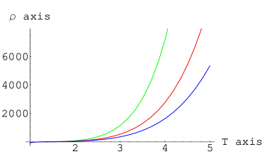
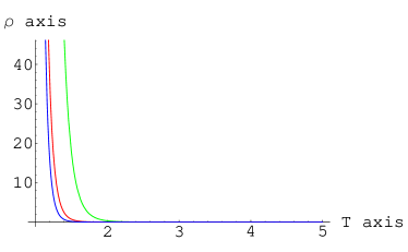
Figure 1: Plots represent energy density $\rho$ versus time T for $\alpha<\frac{2(m+2)}{3}$ and $\alpha>\frac{2(m+2)}{3}$ respectively. Here $\omega_{0}=1.9,~{}n=2$ and $\alpha=1$.

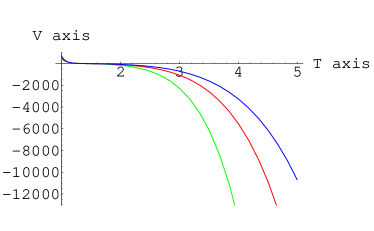
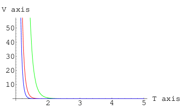
Figure 2: The self-interacting potential $U(T)$ versus time T for $\alpha<\frac{2(m+2)}{3}$ and $\alpha>\frac{2(m+2)}{3}$. Here $\omega_{0}=-1.9,~{}\beta=2,n=-2,~{}\alpha=1$.

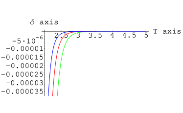
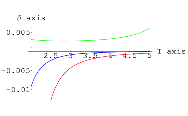
Figure 3: The skewness parameter $\delta(T)$ for $\alpha<\frac{2(m+2)}{3}$ and $\alpha>\frac{2(m+2)}{3}$ respectively. Here $\omega_{0}=-1.9,~{}\alpha=1,~{}n=2$.

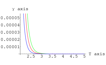
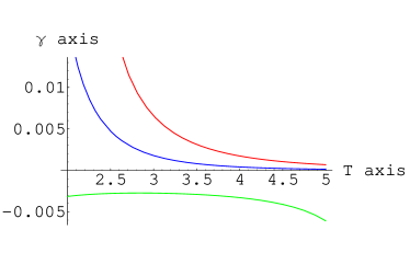
Figure 4: The skewness parameter $\gamma(T)$ for $\alpha<\frac{2(m+2)}{3}$ and $\alpha>\frac{2(m+2)}{3}$ respectively.

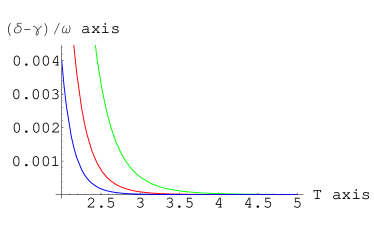
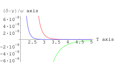
Figure 5: The anisotropic measure of expansion parameter $(\delta-\gamma)/\omega$ for $\alpha<\frac{2(m+2)}{3}$ and $\alpha>\frac{2(m+2)}{3}$ respectively.

Now we discuss the results for $\alpha<\frac{2(m+2)}{3}$ and $\alpha>\frac{2(m+2)}{3}$. Figure 1 indicates that the energy density is positive. For later times, it decreases and goes to zero for $\alpha>\frac{2(m+2)}{3}$ while it increases and approaches to infinity after big bang for $\alpha<\frac{2(m+2)}{3}$. The self-interacting potential is positive only for $\alpha>\frac{2(m+2)}{3}$ as shown in Figure 2 and goes to zero for later times. Figures 3 and 4 show that the skewness parameters $\delta(T)$ and $\gamma(T)$ turn out to be finite at $T=0$ and approach to zero in future evolution of the universe for both cases. The anisotropy measure of expansion for anisotropic fluid goes to zero for $T\rightarrow\infty$ which shows that the anisotropic fluid approaches to isotropy for future evolution of the universe as shown in Figure 5. Notice that all these parameters decrease more rapidly with increasing values of the parameter $m$.

At the initial epoch with $\alpha<\frac{2(m+2)}{3}$ and $\alpha>\frac{2(m+2)}{3}$, we obtain $\omega=-1-\frac{(4+2m+3\alpha)}{(m+2)}$ and $\omega=-1+\frac{8\alpha}{(m+2)(3\alpha-2(m+2))}$ respectively. These indicate that for $m>1$ and $\alpha>0$, the universe may be in phantom region or quintessence region. For later times with $\alpha<\frac{2(m+2)}{3}$, we have $\omega=-1+\frac{8\alpha}{(m+2)(3\alpha-2(m+2))}$ and for $\alpha>\frac{2(m+2)}{3}$, it follows that

$$\omega = -1-\frac{1}{(m+2)}[[\phi_{0}\alpha(m+2)((3+2\omega_{0})\alpha(\alpha+m+1)+4(1+2m)$$

$$+ 4\alpha(m+2)-2\omega_{0}\alpha^{2})-(\alpha-2+\frac{8\alpha(m+2)}{(3\alpha-2(m+2))})\frac{\phi_{0}\alpha^{2}(m+2)}{2}$$

$$\times (3+2\omega_{0})][-2(\alpha+2m+4)]+\alpha^{2}\phi_{0}\frac{(3+2\omega_{0})(m+2)}{(3\alpha-2(m+2))}[-(\alpha+2m$$

$$+ 4)][[\phi_{0}\alpha(m+2)((3+2\omega_{0})\alpha(\alpha+m+1)+4(1+2m)+4\alpha(m+2)$$

$$- 2\omega_{0}\alpha^{2})-\frac{\phi_{0}\alpha^{2}(m+2)(3+2\omega_{0})}{2}(\frac{8\alpha(m+2)}{(3\alpha-2(m+2))}+\alpha-2)][2$$

$$\times (8\alpha(m+2)-(\alpha+2m+4)(3\alpha-2(m+2)))^{-1}]$$

$$+ \alpha^{2}\phi_{0}\frac{(3+2\omega_{0})(m+2)}{(3\alpha-2(m+2))}]^{-1}.$$

This also shows that the universe will be in quintessence region or phantom region for later times depending on the value of the BD parameter. Thus the model represents accelerated expansion of the universe.

4 Magnetized Anisotropic Fluid Model

In this section, we explore solution of the field equations for magnetized anisotropic fluid. We take anisotropic fluid with magnetic field along $z$ axis and assume that there is no electric field. In this case, the scale factor $A(t)$ is perpendicular to magnetic field while $B(t)$ is along the field lines. The magnetized anisotropic fluid is

$$T^{\nu}_{\mu}=diag[\rho+\rho_{B},-p_{x}+\rho_{B},-p_{y}-\rho_{B},-p_{z}-\rho_{B}],$$ (39)

where $\rho_{B}$ represents energy density of the magnetic field. Using EoS for pressures in $x,~{}y$ and $z$ directions as in the anisotropic fluid, Eq.(39) can be written as

$$T^{\nu}_{\mu}=diag[\rho+\rho_{B},-(\omega+\delta)+\rho_{B},-(\omega+\gamma)-\rho_{B},-(\omega+\gamma)-\rho_{B}],$$ (40)

where $\delta$ and $\gamma$ are given by Eq.(26). For $\delta=0=\gamma$, Eq.(40) corresponds to the energy-momentum tensor for the magnetized isotropic fluid while it reduces to the anisotropic fluid for $\rho_{B}=0$. For $\delta=0=\gamma$ and $\rho_{B}=0$, it represents the isotropic fluid.

The field equations (2) and (3) for the model (4) and the energy-momentum tensor (40) become

$$(2m+1)\frac{\dot{B}^{2}}{B^{2}} = \frac{\rho+\rho_{B}}{\phi}+\frac{\omega_{0}}{2}\frac{\dot{\phi}^{2}}{\phi^{2}}-(m+2)\frac{\dot{B}}{B}\frac{\dot{\phi}}{\phi}+\frac{U(\phi)}{2\phi},$$ (41)

$$2\frac{\ddot{B}}{B}+\frac{\dot{B}^{2}}{B^{2}} = -\frac{(\omega+\delta)\rho-\rho_{B}}{\phi}-\frac{\omega_{0}}{2}\frac{\dot{\phi}^{2}}{\phi^{2}}-2\frac{\dot{B}}{B}\frac{\dot{\phi}}{\phi}-\frac{\ddot{\phi}}{\phi}$$ (42)

$$+ \frac{U(\phi)}{2\phi},$$

$$(m+1)\frac{\ddot{B}}{B}+m^{2}\frac{\dot{B}^{2}}{B^{2}} = -\frac{(\omega+\gamma)\rho+\rho_{B}}{\phi}-\frac{\omega_{0}}{2}\frac{\dot{\phi}^{2}}{\phi^{2}}-\frac{\ddot{\phi}}{\phi}$$ (43)

$$- (m+1)\frac{\dot{B}}{B}\frac{\dot{\phi}}{\phi}+\frac{U(\phi)}{2\phi},$$

$$\ddot{\phi}+(m+2)\frac{\dot{B}}{B}\dot{\phi} = \frac{\rho(1-3\omega)-\rho(\delta+2\gamma)}{(2\omega_{0}+3)}-\frac{2U(\phi)-\phi\frac{dU}{d\phi}}{(2\omega_{0}+3)},$$ (44)

where we have used the condition $A=B^{m}$.

The energy conservation equation for the magnetized anisotropic fluid yields $\rho_{B}=\frac{\beta}{B^{4}}$ along with Eq.(24). Here $\beta>0$ is an integration constant. Subtraction of Eq.(42) from (43) leads to

$$2\frac{\ddot{B}}{B}+2(m+1+\alpha)(\frac{\dot{B}^{2}}{B^{2}})-\frac{2n(m+2)^{2}}{3\phi_{0}(m-1)B^{\alpha}}(\frac{\dot{B}^{2}}{B^{2}})=-\frac{4\beta}{\phi_{0}(m-1)B^{\alpha+4}}.$$ (45)

Taking $\dot{B}=f(B)$, this turns out to be

$$\frac{df^{*}}{dB}+\frac{2}{B}[(m+1+\alpha)-\frac{nl}{3\phi_{0}(m-1)B^{\alpha}}]f^{*}=\frac{-4\beta}{\phi_{0}(m-1)B^{\alpha+3}},$$ (46)

where $f^{*}=f^{2}$ and $l=(m+2)^{2}$ is a positive constant. This is the first-order linear non-homogeneous differential equation with variable coefficients whose integrating factor is $B^{2(m+1+\alpha)}e^{\frac{2nlB^{-\alpha}}{3\phi_{0}\alpha(m-1)}}$. After some manipulation, the solution becomes

$$f^{2}=\dot{B}^{2} = \frac{-4\beta B^{-(\alpha+2)}}{\phi_{0}(\alpha+2m)(m-1)}-\frac{4nl\beta B^{-2(\alpha+1)}}{3m(m-1)^{2}\phi_{0}^{2}(\alpha+2m)}$$ (47)

$$\times (1-\frac{2nlB^{-\alpha}}{3\phi_{0}(m-1)\alpha})+c_{2}B^{-2(m+1+\alpha)}(1-\frac{2nlB^{-\alpha}}{3\phi_{0}(m-1)\alpha}),$$

where $c_{2}$ is an integration constant. This can also be written as

$$dt = \int[\frac{-4\beta B^{-(\alpha+2)}}{\phi_{0}(\alpha+2m)(m-1)}-\frac{4nl\beta B^{-2(\alpha+1)}}{3m(m-1)^{2}\phi_{0}^{2}(\alpha+2m)}$$

$$\times (1-\frac{2nlB^{-\alpha}}{3\phi_{0}(m-1)\alpha})+c_{2}B^{-2(m+1+\alpha)}(1-\frac{2nlB^{-\alpha}}{3\phi_{0}(m-1)\alpha})]^{-1/2}dB.$$

By taking $B=T,~{}x=X,~{}y=Y$ and $z=Z$ and using Eq.(47), BI spacetime turns out to be

$$ds^{2} = [\frac{-4\beta T^{-(\alpha+2)}}{\phi_{0}(\alpha+2m)(m-1)}-\frac{4nl\beta T^{-2(\alpha+1)}}{3m(m-1)^{2}\phi_{0}^{2}(\alpha+2m)}$$ (48)

$$\times (1-\frac{2nlT^{-\alpha}}{3\phi_{0}(m-1)\alpha})+c_{2}T^{-2(m+1+\alpha)}(1-\frac{2nlT^{-\alpha}}{3\phi_{0}(m-1)\alpha})]^{-1}dT^{2}$$

$$- T^{2m}dX^{2}-T^{2}(dY^{2}+dZ^{2}).$$

Now we discuss some physical features of this model. Since at $T=0$, the scale factors will be zero, the model shows point type singularity [18, 22]. The corresponding mean and directional Hubble parameters are

$$H_{x}=mH_{y} = m[\frac{-4\beta T^{-(\alpha+4)}}{\phi_{0}(\alpha+2m)(m-1)}-\frac{4nl\beta T^{-2(\alpha+2)}}{3m(m-1)^{2}\phi_{0}^{2}(\alpha+2m)}$$

$$\times (1-\frac{2nlT^{-\alpha}}{3\phi_{0}(m-1)\alpha})+c_{2}T^{-2(m+2+\alpha)}(1-\frac{2nlT^{-\alpha}}{3\phi_{0}(m-1)\alpha})]^{1/2},$$

$$H = \frac{(m+2)}{3}[\frac{-4\beta T^{-(\alpha+4)}}{\phi_{0}(\alpha+2m)(m-1)}-\frac{4nl\beta T^{-2(\alpha+2)}}{3m(m-1)^{2}\phi_{0}^{2}(\alpha+2m)}$$

$$\times (1-\frac{2nlT^{-\alpha}}{3\phi_{0}(m-1)\alpha})+c_{2}T^{-2(m+2+\alpha)}(1-\frac{2nlT^{-\alpha}}{3\phi_{0}(m-1)\alpha})]^{1/2}.$$

Since $\alpha,~{}m>0~{}(m\neq 1)$, these parameters increase with the decrease in $T$ and approach to zero as $T\rightarrow\infty$. Also, these parameters take infinitely large values at $T=0$. The remaining parameters are given by

$$\Theta = 3H=(m+2)[\frac{-4\beta T^{-(\alpha+4)}}{\phi_{0}(\alpha+2m)(m-1)}-\frac{4nl\beta T^{-2(\alpha+2)}}{3m(m-1)^{2}\phi_{0}^{2}(\alpha+2m)}$$ (51)

$$\times (1-\frac{2nlT^{-\alpha}}{3\phi_{0}(m-1)\alpha})+c_{2}T^{-2(m+2+\alpha)}(1-\frac{2nlT^{-\alpha}}{3\phi_{0}(m-1)\alpha})]^{1/2},$$

$$\sigma^{2} = \frac{(m-1)^{2}}{3}[\frac{-4\beta T^{-(\alpha+4)}}{\phi_{0}(\alpha+2m)(m-1)}-\frac{4nl\beta T^{-2(\alpha+2)}}{3m(m-1)^{2}\phi_{0}^{2}(\alpha+2m)}$$ (52)

$$\times (1-\frac{2nlT^{-\alpha}}{3\phi_{0}(m-1)\alpha})+c_{2}T^{-2(m+2+\alpha)}(1-\frac{2nlT^{-\alpha}}{3\phi_{0}(m-1)\alpha})],$$

$$q = -(1-\frac{3}{(m+2)})-\frac{3}{2(m+2)}[\frac{-4\beta T^{-(\alpha+4)}}{\phi_{0}(\alpha+2m)(m-1)}-\frac{4nl\beta}{3m(m-1)^{2}}$$

$$\times \frac{T^{-2(\alpha+2)}}{\phi_{0}^{2}(\alpha+2m)}(1-\frac{2nlT^{-\alpha}}{3\phi_{0}(m-1)\alpha})+c_{2}T^{-2(m+2+\alpha)}(1-\frac{2nl\phi_{0}^{-1}}{3(m-1)\alpha}$$

$$\times T^{-\alpha})]^{-1/2}(\frac{-4\beta B^{-(\alpha+2)}}{\phi_{0}(\alpha+2m)(m-1)}-\frac{4nl\beta B^{-2(\alpha+1)}}{3m(m-1)^{2}\phi_{0}^{2}(\alpha+2m)}$$

$$\times (1-\frac{2nlB^{-\alpha}}{3\phi_{0}(m-1)\alpha})+c_{2}B^{-2(m+1+\alpha)}(1-\frac{2nlB^{-\alpha}}{3\phi_{0}(m-1)\alpha}))^{-1/2}$$

$$\times (\frac{4(\alpha+2)\beta B^{-(\alpha+3)}}{\phi_{0}(\alpha+2m)(m-1)}+\frac{8(\alpha+1)nl\beta B^{-(2\alpha+3)}}{3m(m-1)^{2}\phi_{0}^{2}(\alpha+2m)}$$

$$\times (1-\frac{2nlB^{-\alpha}}{3\phi_{0}(m-1)\alpha})-\frac{4nl\beta B^{-2(\alpha+1)}}{3m(m-1)^{2}\phi_{0}^{2}(\alpha+2m)}(\frac{2nl\alpha B^{-(\alpha+1)}}{3\phi_{0}(m-1)\alpha})$$

$$- 2c_{2}(m+1+\alpha)B^{-(2m+3+2\alpha)}(1-\frac{2nlB^{-\alpha}}{3\phi_{0}(m-1)\alpha})$$

$$+ c_{2}B^{-2(m+1+\alpha)}(\frac{2nl\alpha B^{-(\alpha+1)}}{3\phi_{0}(m-1)\alpha})).$$

In this case, the volume of the universe and anisotropic parameter of expansion turn out to be the same as in anisotropic case. For initial time, the expansion and shear scalar become infinite while for later times, these decrease to zero. The deceleration parameter turns out to be a dynamical quantity. It can be negative for appropriate values of the constant parameters e.g., it becomes a negative for later times with $m>1$. Notice that the expansion scalar, shear scalar and Hubble parameters are decreased by the component of magnetic field.

We solve Eqs.(41) and (44) simultaneously to obtain density $\rho$ and the self-interacting potential $U(\phi)\approx U(T)$. The density is

$$\rho(T) = \phi_{0}(1+2m+\alpha(m+2)-\frac{\omega_{0}\alpha^{2}}{2})[\frac{-4\beta T^{-4}}{(\alpha+2m)(m-1)\phi_{0}}$$ (53)

$$- \frac{4nl\beta}{3m(m-1)^{2}}\frac{T^{-(\alpha+4)}}{(\alpha+2m)\phi_{0}^{2}}(1-\frac{2nlT^{-\alpha}}{3\phi_{0}(m-1)\alpha})$$

$$+ c_{2}T^{-(4+2m+\alpha)}(1-\frac{2nlT^{-\alpha}}{3\phi_{0}(m-1)\alpha})]-\frac{\beta}{T^{4}}-\frac{U(T)}{2},$$

where $U(T)$ is

$$U(T) = [((2\omega_{0}+3)(\alpha+m+1)\alpha^{2}-4\alpha(1+2m+\alpha(m+2)-\frac{\omega_{0}\alpha^{2}}{2}))2(m$$

$$+ 2)+\alpha^{2}(m+2)(3+2\omega_{0})(\frac{8\alpha(m+2)}{2(m+2)-3\alpha}-(\alpha-2))-6\alpha(1+2m$$

$$+ \alpha(m+2)-\frac{\omega_{0}\alpha^{2}}{2})\frac{8\alpha(m+2)}{2(m+2)-3\alpha}][4\beta T^{-4}[(\alpha+2m)(m-1)\phi_{0}(8\alpha$$

$$\times (m+2)+4(2(m+2)-3\alpha))]^{-1}-\frac{4\beta nl}{3m(\alpha+2m)(m-1)^{2}\phi_{0}^{2}}$$

$$\times (-T^{-(\alpha+4)}[(8\alpha(m+2)+(\alpha+4)(2(m+2)-3\alpha))]^{-1}+\frac{2}{3}nl\phi_{0}^{-1}(m$$ (54)

$$- 1)^{-1}T^{-(2\alpha+4)}(8\alpha^{2}(m+2)+2\alpha(\alpha+2)(2(m+2)-3\alpha))^{-1}-c_{2}(8\alpha$$

$$\times (m+2)-(\alpha+2m+4)(2(m+2)-3\alpha))^{-1}T^{-(4+2m+\alpha)}+\frac{2}{3}nl\phi_{0}^{-1}$$

$$\times (m-1)^{-1}\alpha T^{-(2\alpha+2m+4)}(8\alpha(m+2)+2(\alpha+m+2)(2(m+2)$$

$$- 3\alpha))^{-1}+\frac{\alpha^{2}(2\omega_{0}+3)}{(2(m+2)-3\alpha)}[\frac{-4(m+2)\beta T^{-4}}{(\alpha+2m)(m-1)\phi_{0}}-\frac{4(m+2)}{3m(m-1)^{2}}$$

$$\times \frac{\beta nl}{(\alpha+2m)}(T^{-(\alpha+4)}-\frac{2nlT^{-2(\alpha+2)\phi_{0}^{-1}}}{3\alpha(m-1)})+c_{2}(m+2)(T^{-(\alpha+2m+4)}$$

$$- \frac{2nl\phi_{0}^{-1}}{3\alpha(m-1)}T^{-(2\alpha+2m+4)}]+\frac{4n(m+2)^{2}(1-m)\alpha}{3}[\frac{4\beta T^{-(\alpha+4)}\phi_{0}^{-1}}{(\alpha+2m)(m-1)}$$

$$\times (8\alpha(m+2)+(\alpha+4)(2(m+2)-3\alpha))^{-1}-\frac{4\beta nl\phi_{0}^{-2}}{3m(\alpha+2m)(m-1)^{2}}$$

$$\times (-T^{-(2\alpha+4)}(8\alpha(m+2)+(2\alpha+4)(2(m+2)-3\alpha))^{-1}$$

$$+ \frac{2nlT^{-(3\alpha+4)}}{3\phi_{0}(m-1)\alpha}(8\alpha(m+2)+(3\alpha+4)(2(m+2)-3\alpha))^{-1}$$

$$+ c_{2}(-T^{-(4+2m+2\alpha)}(8\alpha(m+2)+(2\alpha+2m+4)(2(m+2)-3\alpha))^{-1}$$

$$+ \frac{2nlT^{-(3\alpha+2m+4)}}{3\phi_{0}(m-1)\alpha}(8\alpha(m+2)+(3\alpha+2m+4)(2(m+2)-3\alpha))^{-1})$$

$$- 8\alpha\beta(m+2)T^{-4}(8\alpha(m+2)+4(2(m+2)-3\alpha))^{-1}+6\alpha(2(m+2)$$

$$- 3\alpha)_{-1}[\beta T^{-4}-8\beta\alpha(m+2)T^{-4}(8\alpha(m+2)+4(2(m+2)-3\alpha))^{-1}]$$

$$- \frac{6\alpha}{(2(m+2)-3\alpha)}(1+2m+\alpha(m+2)-\frac{\omega_{0}\alpha^{2}}{2})[\frac{-4\beta T^{-(\alpha+3)}}{(\alpha+2m)(m-1)}$$

$$- \frac{4\beta nl}{3m(m-1)^{2}(\alpha+2m)}(T^{-(2\alpha+3)}-\frac{2nlT^{-3(\alpha+1)}}{3\phi_{0}(m-1)\alpha})+c_{2}(T^{-(2\alpha+2m+3)}$$

$$- \frac{2nlT^{-(3\alpha+2m+3)}}{3\alpha(m-1)\phi_{0}})]+c_{3}T^{\frac{8\alpha(m+2)}{2(m+2)-3\alpha}},$$

where $c_{3}$ is an integration constant. Figure 6 indicates that the energy density is positive and decreases after big bang but it increases and approaches to infinity for later times with $\alpha<\frac{2(m+2)}{3}$. The energy density is positive but decreases to zero for any positive value of the parameter satisfying $\alpha>\frac{2(m+2)}{3}$ as shown in Figure 6. At the initial epoch, there is infinite energy density in both cases as shown in Figure 6. Figures 7 indicate that the self-interacting potential remains positive in both cases ($\alpha<\frac{2(m+2)}{3}$ and $\alpha>\frac{2(m+2)}{3}$). The corresponding skewness parameters turn out to be

$$\delta(T) = \frac{2n(m+2)}{3\rho}[\frac{-4\beta T^{-(\alpha+4)}}{(\alpha+2m)(m-1)\phi_{0}}-\frac{4nl\beta T^{-2(\alpha+2)}}{3m(m-1)^{2}(\alpha+2m)\phi_{0}^{2}}$$ (55)

$$\times (1-\frac{2nlT^{-\alpha}}{3\phi_{0}(m-1)\alpha})+c_{2}T^{-2(2+m+\alpha)}(1-\frac{2nlT^{-\alpha}}{3\phi_{0}(m-1)\alpha})],$$

$$\gamma(T) = \frac{-nm(m+2)}{3\rho}[\frac{-4\beta T^{-(\alpha+4)}}{(\alpha+2m)(m-1)\phi_{0}}-\frac{4nl\beta T^{-2(\alpha+2)}}{3m(m-1)^{2}(\alpha+2m)\phi_{0}^{2}}$$ (56)

$$\times (1-\frac{2nlT^{-\alpha}}{3\phi_{0}(m-1)\alpha})+c_{2}T^{-2(2+m+\alpha)}(1-\frac{2nlT^{-\alpha}}{3\phi_{0}(m-1)\alpha})],$$

where $\rho$ is given by Eq.(53). Figures 8 and 9 indicate that the deviation parameters become finite at $T=0$. For later times, these parameters converge to zero in both cases. From Eqs.(24) and (25), the deviation free EoS parameter $\omega$ can be written as

$$\omega(T)=-1-\frac{B}{\rho(m+2)}\frac{d\rho}{dB}.$$ (57)

The anisotropy measure of anisotropic fluid, $\frac{\delta-\gamma}{\omega}$, for the model (48) takes the form

$$\frac{\delta-\gamma}{\omega} = \frac{n(m+2)^{2}}{3\omega(T)}[\frac{-4\beta T^{-(\alpha+4)}}{(\alpha+2m)(m-1)\phi_{0}}-\frac{4nl\beta T^{-2(\alpha+2)}}{3m(m-1)^{2}(\alpha+2m)\phi_{0}^{2}}$$ (58)

$$\times (1-\frac{2nlT^{-\alpha}}{3\phi_{0}(m-1)\alpha})+c_{2}T^{-2(2+m+\alpha)}(1-\frac{2nlT^{-\alpha}}{3\phi_{0}(m-1)\alpha})].$$

Its behavior is shown in Figure 10.

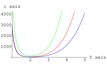
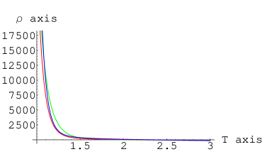
Figure 6: Plots represent the energy density $\rho(T)$ versus time T for $\alpha<\frac{2(m+2)}{3}$ and $\alpha>\frac{2(m+2)}{3}$ respectively. Here $\omega_{0}=-1.9,~{}\beta=2,~{}n=-2$. Green, red and blue lines show the graphs for $m=2,3,4$ respectively.

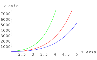
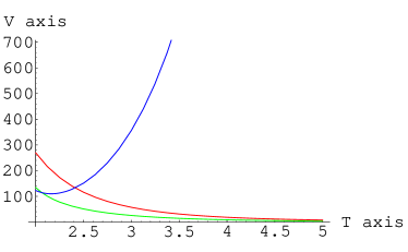
Figure 7: Plots show the self-interacting potential $U(T)$ versus time T for $\alpha<\frac{2(m+2)}{3}$ and $\alpha>\frac{2(m+2)}{3}$ respectively.

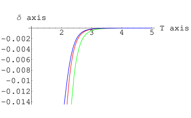
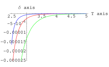
Figure 8: The deviation parameter $\delta(T)$ versus time T for $\alpha<\frac{2(m+2)}{3}$ and $\alpha>\frac{2(m+2)}{3}$ respectively. Here $\omega_{0}=-1.9,~{}\beta=2$ and $n=-2$.

For initial epoch, this is finite while it goes to zero for the future evolution of the universe in both cases. This indicates that the anisotropic fluid approaches to isotropy for later times. When $T\longrightarrow 0$ and $\alpha<\frac{2(m+2)}{3}$, we obtain $\omega=-1-\frac{(4+2m+3\alpha)}{(m+2)}$ which shows that the universe model will be in phantom region at initial epoch. For $\alpha>\frac{2(m+2)}{3}$, we obtain $\omega=-1+\frac{8\alpha}{(m+2)(3\alpha-2(m+2))}$ which shows that the universe model will be in quintessence region at initial epoch. For later times with $\alpha<\frac{2(m+2)}{3}$, it follows that $\omega=-1+\frac{8\alpha}{(m+2)(3\alpha-2(m+2))}$ showing that the universe may be in quintessence region. When $\alpha>\frac{2(m+2)}{3}$, the EoS parameter depends on the component of magnetic field and BD parameter indicating that the universe will be in phantom or quintessence region for appropriate values of the constant parameters. Thus, in each case, the model shows the accelerated expansion of the universe.

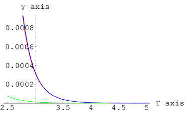
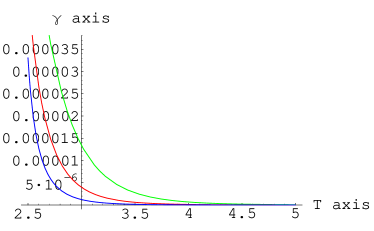
Figure 9: The deviation parameter $\gamma(T)$ versus time T for $\alpha<\frac{2(m+2)}{3}$ and $\alpha>\frac{2(m+2)}{3}$ respectively.

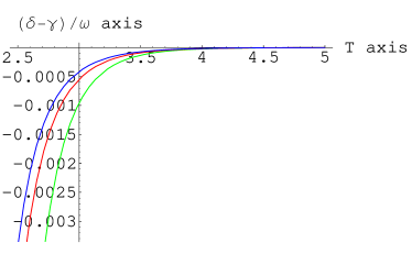
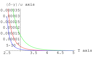
Figure 10: Anisotropic measure of expansion $\frac{\delta-\gamma}{\omega}$ versus time T is shown for $\alpha<\frac{2(m+2)}{3}$ and $\alpha>\frac{2(m+2)}{3}$ respectively.

Now we investigate a special case when $m=1$. The scale factors become $A(t)=B(t)=a(t)$ and the model turns out to be the FRW universe model

$$ds^{2}=dt^{2}-a(t)^{2}(dx^{2}+dy^{2}+dz^{2}).$$

Equation (45) yields

$$a(t)=\sqrt{2}(\sqrt{\frac{2\beta}{3n}}t+c_{4})^{1/2},$$ (59)

where $c_{4}$ is an integration constant. The expansion scalar $\Theta$ turns out to be

$$\Theta=3H=3(\frac{\dot{a}}{a})=3\sqrt{\frac{2\beta}{3n}}(\sqrt{\frac{2\beta}{3n}}t+c_{4})^{-1}.$$

This shows that the Hubble parameter and the expansion scalar are constant at earlier time. As time increases, both of these parameters decrease indicating expanding universe in its earlier time. From Eqs.(41) and (44), the energy density $\rho(t)$ and the self-interacting potential $U(t)$ are

$$\rho(t) = S_{1}[\sqrt{\frac{2\beta}{3n}}t+c_{4}]^{\frac{\alpha-2}{2}}+S_{2}[\sqrt{\frac{2\beta}{3n}}t+c_{4}]^{\frac{\alpha-4}{2}}+c_{5}[2(\sqrt{\frac{2\beta}{3n}}t$$

$$+ c_{4})]^{\frac{4\alpha}{(2-\alpha)}}-\frac{\beta}{4}[\sqrt{\frac{2\beta}{3n}}t+c_{4}]^{-2},$$

$$U(t) = -[2\phi_{0}\alpha((3+2\omega_{0})\alpha(\alpha+2)-12(1+\alpha)+2\omega_{0}\alpha^{2})+\frac{\alpha^{2}(3+2\omega_{0})}{(2-\alpha)}$$

$$\times \phi_{0}(\alpha+2)^{2}-\frac{16\phi_{0}\alpha^{2}}{(2-\alpha)}(3(1+\alpha)-\frac{\omega_{0}\alpha^{2}}{2})][\sqrt{\frac{2\beta}{3n}}t+c_{4}]^{\frac{\alpha-2}{2}}(\frac{2\beta}{3n})^{3/2}$$

$$\times (\alpha+2)^{-2}+[\frac{2^{(\alpha-2)/2}\phi_{0}\alpha^{2}(3+2\omega_{0})\beta}{3n(2-\alpha)}-\frac{4\alpha\phi_{0}\beta 2^{\alpha/2}}{3n(2-\alpha)}(3(1+\alpha)$$

$$- \frac{\omega_{0}\alpha^{2}}{2})][\sqrt{\frac{2\beta}{3n}}t+c_{4}]^{\frac{\alpha-4}{2}}+c_{5}[2(\sqrt{\frac{2\beta}{3n}}t+c_{4})]^{\frac{4\alpha}{(2-\alpha)}}.$$

Here $c_{5}$ is an integration constant and the constants $S_{1}$ and $S_{2}$ are given by

$$S_{1} = -(1/2)[2\phi_{0}\alpha((3+2\omega_{0})\alpha(\alpha+2)-12(1+\alpha)+2\omega_{0}\alpha^{2})$$

$$+ \frac{\alpha^{2}(3+2\omega_{0})\phi_{0}}{(2-\alpha)}(\alpha+2)^{2}-\frac{16\phi_{0}\alpha^{2}}{(2-\alpha)}(3(1+\alpha)-\frac{\omega_{0}\alpha^{2}}{2})]$$

$$\times (\frac{2\beta}{3n})^{3/2}(\alpha+2)^{-2},$$

$$S_{2} = [\frac{2^{(\alpha-2)/2}\phi_{0}\alpha^{2}(3+2\omega_{0})\beta}{6n(2-\alpha)}-\frac{4\alpha\phi_{0}\beta 2^{\alpha/2}}{6n(2-\alpha)}(3(1+\alpha)-\frac{\omega_{0}\alpha^{2}}{2})$$

$$+ \phi_{0}(3(1+\alpha)-\frac{\omega_{0}\alpha^{2}}{2})\frac{2^{(\alpha-2)/2}\beta}{3n}].$$

Some other parameters are

$$\delta(t) = \frac{4\beta}{3\rho}(\sqrt{\frac{2\beta}{3n}}t+c_{4})^{-2},\quad\gamma(t)=\frac{-2\beta}{3\rho}(\sqrt{\frac{2\beta}{3n}}t+c_{4})^{-2},$$

$$\omega(t) = -1-[\frac{S_{1}(\alpha-2)}{2}(\sqrt{\frac{2\beta}{3n}}t+c_{4})^{(\alpha-4)/2}+\frac{S_{2}(\alpha-4)}{2}(\sqrt{\frac{2\beta}{3n}}t$$

$$+ c_{4})^{(\alpha-6)/2}+c_{5}2^{4\alpha/(2-\alpha)}(\frac{4\alpha}{(2-\alpha)}\sqrt{\frac{2\beta}{3n}}t+c_{4})^{(5\alpha-2)/(2-\alpha)}$$

$$+ \frac{\beta}{2}(\sqrt{\frac{2\beta}{3n}}t+c_{4})^{-3}][3S_{1}[\sqrt{\frac{2\beta}{3n}}t+c_{4}]^{\frac{\alpha-4}{2}}+3S_{2}[\sqrt{\frac{2\beta}{3n}}t+c_{4}]^{\frac{\alpha-6}{2}}$$

$$+ 3c_{5}2^{4\alpha/(2-\alpha)}[2(\sqrt{\frac{2\beta}{3n}}t+c_{4})]^{\frac{(5\alpha-2)}{(2-\alpha)}}-\frac{\beta}{4}[\sqrt{\frac{2\beta}{3n}}t+c_{4}]^{-3}]^{-1},$$

$$\frac{\delta-\gamma}{\omega} = \frac{2\beta(\sqrt{\frac{2\beta}{3n}}t+c_{4})^{-2}}{\omega(t)},$$

where $\alpha\neq 2$. We discuss two cases: $0<\alpha<2$ and $\alpha>2$. Clearly, the energy density is constant at initial epoch and approaches to infinity for later times in both cases. The anisotropy parameters are constant at initial epoch and go to zero for later times. Likewise the anisotropy measure of expansion of anisotropic fluid $\frac{\delta-\gamma}{\omega}$ approaches to isotropy for later times. The anisotropy parameter of expansion is zero as $m=1$. At the initial epoch, the deviation free EoS parameter shows that the universe may be in quintessence region by choosing appropriate values of the constants in both cases. For later times with $0<\alpha<2$, we obtain $\omega(t)=-1-\frac{4\alpha}{3(2-\alpha)}$ which indicates that the universe will be in phantom region. For $\alpha>2$, it follows that $\omega(t)=-1-\frac{(\alpha-2)}{6}$, which also shows that the universe will be in phantom region for future evolution.

5 Summary and Discussion

In this paper, we have constructed the BI universe models in BD theory of gravity with perfect, anisotropic and magnetized anisotropic fluids. We have constructed exact solutions in each case. For anisotropic and anisotropic magnetized fluid models, the physical behavior of the energy density, self-interacting potential, skewness parameters and anisotropy parameter of expansion of anisotropy fluid have been plotted for non-zero value of $n$ with $\alpha<\frac{2(m+2)}{3}$ and $\alpha>\frac{2(m+2)}{3}$. The results are summarized as follows.

• In the case of anisotropic as well as magnetized anisotropic fluids, the skewness parameters and anisotropic measure of expansion of anisotropic fluid go to zero indicating the isotropic behavior of the fluid for the future evolution of the universe. This result coincides with those already available in literature for Bianchi type III model in $f(R)$ theory [11] and Bianchi type $(VI)_{0}$ model in GR [23].

• In each case, the energy density remains positive. All the figures indicate that energy density increases after big bang and approaches to infinity for later times with $\alpha<\frac{2(m+2)}{3}$ in both anisotropic as well as magnetized anisotropic fluids. For $\alpha>\frac{2(m+2)}{3}$, it decreases and goes to zero in both cases.

• For anisotropic fluid, the self interacting potential is positive only for $\alpha>\frac{2(m+2)}{3}$ and decreases to zero for later times while for magnetized anisotropic fluid, it remains positive in both cases.

• All the physical parameters $H,~{}H_{x},H_{y},~{}\Theta$ and $\sigma$ increase with the decrease in $T$ and go to zero as $T\rightarrow\infty$. These parameters take infinitely large values at $T=0$. In contrast to the perfect fluid, the deceleration parameter for anisotropic fluids is a dynamical quantity and can be negative for the appropriate choice of constant parameters, in particular for later times with $m>1$. This corresponds to accelerated expansion of the universe.

• In the anisotropic magnetized fluid, all the physical parameters are reduced by the component of magnetic field with $n>0$.

• The deviation free EoS parameters indicate that the universe may be in quintessence or phantom region at initial epoch as well as for later times for an appropriate values of the constant parameters in all cases. Thus the models represent the accelerated expansion of the universe.

• The anisotropy parameter of expansion is constant (vanishes for $m=1$) indicating the model does not isotropize for later times in all cases.

• A special case $m=1$ for the magnetized anisotropic fluid has also been discussed which yields FRW universe model. In this case, the deviation free EoS parameter indicates that at initial epoch, the universe may be in quintessence region while for the future evolution, it will be in phantom region.

It would be interesting to construct exact solutions in the presence of anisotropic fluid for other Bianchi models in BD theory.

References

[1] Perlmutter, S. et al.: Astrophys. J. 483(1997)565;
Nature 391(1998)51; Astrophys. J. 517(1999)565;
Riess, A.G. et al.: Astron. J. 116(1998)1009; Bennett, C.L.
et al.: Astrophys. J. Suppl. 148(2003)1; Spergel, D.N. et
al.: Astrophys. J. Suppl. 148(2003)175; Tegmark, M. et al.:
Phys. Rev. D69(2004)03501.
[2] Caldwell, R.R., Dave, R. and Steinhardt, P.J.: Phys. Rev. Lett. 80(1998)1582;
Caldwell, R.R.: Phys. Lett. B23(2002)545; Bertolami, O. and
Sen, A.A.: Phys. Rev. D66(2002)043507.
[3] Lobo, F.S.N.: The Dark Side of Gravity: Modified Theories of Gravity, invited
chapter to appear in an edited collection ”Dark Energy-Current
Advances and Ideas”; arXiv:0807.1640; Flanagan, E.E.: Class.
Quantum Grav. 21(2004)417.
[4] Bertolami, O. and Martins, P.J.: Phys. Rev.
D61(2000)064007; Banerjee, N. and Pavon, D.: Phys. Rev.
D63(2001)043504.
[5] Brans, C.H. and Dicke, R.H.: Phys. Rev. 124(1961)925.
[6] Weinberg, S.: Gravitation and Cosmology (Wiley, 1972).
[7] Bertotti, B., Iess, L. and Tortora, P.: Nature 425(2003)374;
Felice, A.D. et al.: Phys. Rev. D74(2006)103005.
[8] Chimento, L.P. et al.: Class. Quantum Grav.
14(1997)3363; Pradhan, A. and Pandey, P.: Astrophys. Space
Sci. 301(2006)221.
[9] Rodrigues, D.C.: Phys. Rev. D77(2008)023534;
Koivisto, T. and Mota, D.F.: JCAP 806(2008)18; Astrophys.
J. 679(2008)1.
[10] Yadav, A.K. and Saha, B.: Astrophys. Space Sci. 337(2012)759.
[11] Sharif, M. and Kausar, H.R.: Phys. Lett.
B697(2011)1; Astrophys. Space Sci. 332(2011)463.
[12] Lorenz-Petzold, D.: Phys. Rev. D29(1984)2399;
Astrophys. Space Sci. 114(1985)277; Kumar, S. and Singh,
C.P.: Int. J. Theor. Phys. 47(2008)1722; Lee, S.: Mod.
Phys. Lett. A26(2011) 2159.
[13] Chakraborty, W. and Debnath, U.: Int. J. Theor. Phys. 48(2009)232.
[14] Rama, S.K., and Gosh, S.: Phys. Lett. B383(1996)32.
[15] Banerjee, N. and Sen, S.: Phys. Rev. D56(1997)1334.
[16] Sotiriou, T.P. and Faraoni, V.: Rev. Mod. Phys. 82(2010)451.
[17] Sen, S. and Seshadri, T.R.: Int. J. Mod. Phys. D12(2003)445.
[18] Sharif, M. and Zubair, M.: Astrophys. Space Sci. 330(2010)399.
[19] Collins, C.B., Glass, E.N. and Wilkinson, D.A.: Gen. Relativ. Gravit. 12(1980)805.
[20] Throne, K.S.: Astrophys. J. 148(1967)51;
Kristian, J. and Sachs, R.K.: Astrophys. J. 143(1966)379;
Collins, C.B.: Phys. Lett. A60(1977)397.
[21] Akarsu, O. and Kilinc, C.B.: Gen. Relativ. Gravit. 42(2010)1.
[22] Dunn, K.A. and Tupper, B.O.J.: Astrophys. J. 204(1976)322.
[23] Sharif, M. and Zubair, M.: Int. J. Mod. Phys. D19(2010)1957.